Homodyne detection and optical parametric amplification: a classical approach applied to proposed “loophole-free” Bell tests

Abstract

Recent proposed “loophole-free” Bell tests are discussed in the light of classical models for the relevant features of optical parametric amplification and homodyne detection. The Bell tests themselves are uncontroversial: there are no obvious loopholes that might cause bias and hence, if the world does, after all, obey local realism, no violation of a Bell inequality will be observed. Interest centres around the question of whether or not the proposed criterion for “non-classical” light is valid. If it is not, then the experiments will fail in their initial concept, since both quantum theorists and local realists will agree that we are seeing a purely classical effect. The Bell test, though, is not the only criterion by which the quantum-mechanical and local realist models can be judged. It is suggested that the quantum-mechanical models given in the proposals will also fail in their detailed predictions. If the experiments are extended by including a range of parameter values and by analysing, in addition to the proposed digitised voltage differences, the raw voltages, the models can be compared in their overall performance and plausibility.

Keywords: Bell tests, classical optics, nonlinear optics, homodyne detection, parametric down-conversion, Bell test loopholes, hidden variables, Wigner density

1 Introduction

No test of Bell’s inequalities [1, 2] to date has been free of “loopholes”. This means that, despite the high levels of statistical significance frequently achieved, violations of the inequalities could be the effects of experimental bias of one kind or another, not evidence for the presence of quantum entanglement. Recent proposed experiments by García-Patrón et al [3] and Nha and Carmichael [4] show promise of being genuinely free from such problems. If the world in fact obeys local realism, they should not, therefore, infringe any Bell inequality.

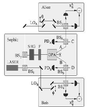
Figure 1: Proposed experimental set-up. In the current text, phase shifts $\theta$ and $\phi$ are renamed $\theta_{A}$ and $\theta_{B}$. For further explanation, see main text. (Reprinted with permission from García-Patrón et al., Phys. Rev. Lett. 93, 130409 (2004). Copyright (2004) by the American Physical Society. )

The current article discusses a classical model that should be able, once all relevant details are known, to explain the results, accounting not only for the failure to infringe the selected Bell test but also for other failures in the detailed predictions. It depends on the classical theory for homodyne detection (re-derived here from first principles) and the known behaviour of (degenerate-mode) optical parametric amplifiers (OPA) [5].

As far as the “loophole-free” status of the proposed experiments is concerned, there would appear to be no problem. A difficulty that seems likely to arise, though, is that theorists may not agree that the test beams used were in fact “non-classical”, so the failure to infringe a Bell inequality will not in itself be interpreted as showing a failure of quantum mechanics. The criterion to be used to establish the non-classical nature of the light is the observation of negative values of the Wigner density, and there is reason to think that, even if the standard method of estimation seems to show that these are achieved, the method may be in error. Wigner density is, in any event, irrelevant to our model. Far from being, as suggested by García-Patrón and others, the “hidden variable” needed, it plays no part whatsoever.

Regardless of the outcome of the Bell tests, and whether or not the light is declared to be non-classical, there are features of the experiments that can usefully be exploited to compare the strengths of quantum mechanics versus (updated) classical theory as viable models. The two theories approach the situation from very different angles. Classical theory traces the causal relationships between phenomena, starting with the simplest assumption and building in random factors later where necessary. Quantum mechanics starts with models of complete ensembles, all random factors included. This, it is argued, is inappropriate, since two features of the proposed experiments demand that we consider the behaviour of individual events, not whole ensembles: the process of homodyne detection itself, and the Bell test.

2 The proposed experiments

The experimental set-up proposed by García-Patrón et al. is shown in Fig. 1, that of Nha and Carmichael being similar. In the words of the García-Patrón et al. proposal:

The source (controlled by Sophie) is based on a master laser beam, which is converted into second harmonic in a nonlinear crystal (SHG). After spectral filtering (F), the second harmonic beam pumps an optical parametric amplifier (OPA) which generates two-mode squeezed vacuum in modes A and B. Single photons are conditionally subtracted from modes A and B with the use of the beam splitters BS_A and BS_B and single-photon detectors PD_A and PD_B. Alice (Bob) measures a quadrature of mode A (B) using a balanced homodyne detector that consists of a balanced beam splitter BS₃ (BS${}_{4})$ and a pair of highly-efficient photodiodes. The local oscillators LO_A and LO_B are extracted from the laser beam by means of two additional beam splitters BS₁ and BS₂.

The classical description, working from the same figure, is just a little different. Quantum theoretical terms such as “squeezed vacuum” and “quadrature” are not used since they are not appropriate to the model and would cause confusion. The description might run as follows:

The master laser beam (which is, incidentally, pulsed) is frequency-doubled in the crystal SHG. After filtering to remove the original frequency, the beam is used to pump the OPA, a resonant cavity containing a nonlinear crystal cut so as to produce degenerate parametric down-conversion of the input. The output comprises pairs of classical wave pulses at half the input frequency, i.e. at the original laser frequency. The selection of pairs for analysis is done by splitting each output at an unbalanced beamsplitter (BS_A or BS${}_{B})$, the smaller parts going to sensitive detectors PD_A or PD_B. Only if there are detections at both PD_A and PD_B is the corresponding homodyne detection included in the analysis. The larger parts proceed to balanced homodyne detectors, i.e. ones in which the intensities of local oscillator and test inputs are approximately equal. The source of the local oscillators LO_A and LO_B is the same laser that stimulated, after frequency doubling, the production of the test beams.

3 Homodyne detection

In (balanced) homodyne detection, the test beam is mixed at a beamsplitter with a local oscillator beam of the same frequency and the two outputs sent to photodetectors that produce voltage readings for every input pulse. In the proposed “loophole-free” Bell tests the difference between the two voltages will be converted into a digital signal by counting all positive values as +1, all negative as –1.

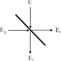
Figure 2: Inputs and outputs at the beamsplitter in a homodyne detector. E_L is the local oscillator beam, E the test beam, E_t and E_r the transmitted and reflected beams respectively.

Assuming the inputs are all classical waves of the same frequency and there are no losses, it can be shown (see below) that the difference between the intensities of the two output beams is proportional to the product of the two input intensities multiplied by $\sin\theta$, where $\theta$ is the phase difference between the test beam and local oscillator. If voltages are proportional to intensities then it follows that the voltage difference will be proportional to $\sin\theta$. When digitised, this transforms to a step function, taking the value $-1$ for $-\pi<\theta<0$ and $+1$ for $0<\theta<\pi$. (The function is not well defined for integral multiples of $\pi$.)

3.1 Classical derivation of the predicted voltage difference

Assume the test and local oscillator signals have the same frequency, $\omega$, the time-dependent part of the test signal being modelled by $e^{i\phi}$, where (ignoring a constant phase offset) $\phi=\omega$t is the phase angle, and the local oscillator phase and test beam phases differ by $\theta$. [Note that although complex notation is used here, only the real part has meaning: this is an ordinary wave equation, not a quantum-mechanical “wave function”. To allay any doubts on this score, the derivation is partially repeated with no complex notation in the Appendix.]

Let the electric fields of the test signal, local oscillator and reflected and transmitted signals from the beamsplitter have amplitudes $E$, $E_{L}$, $E_{r}$ and $E_{t}$ respectively, as shown in Fig. 2. Then, after allowance for phase delays of $\pi/2$ at each reflection and assuming no losses, we have

$$E_{r}=\frac{1}{\sqrt{2}}(Ee^{i(\phi+\pi/2)}+E_{L}e^{i(\phi+\theta)})$$ (1)

and

$$E_{t}=\frac{1}{\sqrt{2}}(Ee^{i\phi}+E_{L}e^{i(\phi+\theta+\pi/2)}).$$ (2)

The intensity of the reflected beam is therefore

$$E_{r}E_{r}^{\ast} = \frac{1}{2}(Ee^{i(\phi+\pi/2)}+E_{L}e^{i(\phi+\theta)})(Ee^{-i(\phi+\pi/2)}$$ (3)

$$+ E_{L}e^{-i(\phi+\theta)})$$

$$= \frac{1}{2}(E^{2}+E_{L}^{2}+EE_{L}e^{i(\pi/2-\theta)}+EE_{L}e^{-i(\pi/2-\theta)})$$

$$= \frac{1}{2}(E^{2}+E_{L}^{2}+2EE_{L}\cos(\pi/2-\theta)$$

$$= \frac{1}{2}(E^{2}+E_{L}^{2}+2EE_{L}\sin\theta).$$

Similarly, it can be shown that the intensity of the transmitted beam is

$$E_{t}E_{t}^{\ast}=\frac{1}{2}(E^{2}+E_{L}^{2}-2EE_{L}\sin\theta).$$ (4)

If the voltages registered by the photodetectors are proportional to the intensities, it follows that the difference in voltage is proportional to $2EE_{L}\sin\theta$. When digitised, this translates to the step function mentioned above. The probabilities for the two possible outcomes are, as shown in Fig. 3,

$$p_{-}=\left\{\begin{array}[]{ll}1&\mbox{for $-\pi<\theta<0$}\\ 0&\mbox{for $0<\theta<\pi$}\end{array}\right.$$ (5)

and

$$p_{+}=\left\{\begin{array}[]{ll}0&\mbox{for $-\pi<\theta<0$}\\ 1&\mbox{for $0<\theta<\pi$}\end{array}\right.$$ (6)

Note that the probabilities are undefined for integral multiples of $\pi$. In practice it would be reasonable to assume that, due to the presence of noise, all the values were 0.5, but for the present purposes the integral values will simply be ignored.

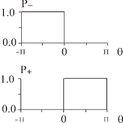
Figure 3: Probabilities of ‘+’ and ‘–’ outcomes versus phase difference, using digitised difference voltages from a perfect, noise-free, balanced homodyne detector.

4 Application to the proposed Bell tests

If the frequencies and phases of both test beams and both local oscillators were all identical apart from the applied phase shifts, the experiments would be expected to produce step function relationships between counts and applied shifts both for the individual (singles) counts and for the coincidences.

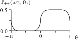
Figure 6: Likely appearance of coincidence curves in a real experiment with moderate noise.

It may safely be assumed that this is not what is observed. It would have shown up in the preliminary trials on the singles counts (see ref. [7]), which would have followed something suggestive of the basic predicted step function as the local oscillator phase shift was varied. What is observed in practice is more likely to be similar to the results obtained by Breitenbach et al. [8]. Their Fig. 6a, reproduced here as Fig. 4, shows a distribution of photocurrents that is clustered around zero, for $\theta$ taking integer multiples of $\pi$, but is scattered fairly equally among positive and negative values in between.

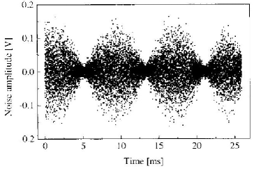
Figure 4: A typical scatter of “noise amplitude” (related to voltage difference) as phase $\theta$ is scanned over time. Minimum scatter occurs for $\theta$ taking integral multiples of $\pi$. (Reprinted from G. Breitenbach et al, J. Opt. Soc. Am. B 12 2304 (1995).)

When digitised, the distribution would reduce to two straight horizontal lines, showing that for each choice of $\theta$ there is an equal chance of a ‘$+$’ or a ‘$-$’ result. As in any other Bell test setup, though, the absence of variations in the singles counts does not necessarily mean there is no variation in the coincidence rates. As explained in the next section, however, the coincidence curves are not the zig-zag ones of standard classical theory. These would be expected if we had full “rotational invariance”. If the ideas presented here are correct, we have instead, in the language of an article by the present author [9], only binary rotational invariance. Breitenbach’s scatter of photocurrent differences is seen as evidence that the relative phase can (under perfect conditions) take just one of two values, 0 or $\pi$. The scatter is formed from a superposition of two sets of points, corresponding to two sine curves that are out of phase, together with a considerable amount of noise.

This interpretation accords well with more comprehensive results of the experiment as reported elsewhere [10]. When part of the initial laser beam is used as “seed” to the OPA, judicious adjustments of the phase can produce “bright squeezed light” and a scatter with alternately positive and negative points. The presence of the seed causes selection of one particular phase set.

The two “phase sets” arise from the way in which the pulses are produced, which involves, after the frequency doubling, the degenerate case of parametric down-conversion, the latter producing pulses that are (in contrast to the general case of conjugate frequencies) of exactly equal frequency. Consider an initial pump laser of frequency $\omega$. In the proposed experiment, this will be doubled in the crystal SHG to 2$\omega$ then halved in the OPA back to $\omega$. At the frequency doubling stage, one laser input wave peak gives rise to two output ones. Assuming that there are causal mechanisms involved, it seems inevitable that every other wave peak of the output will be exactly in phase with the input. When we now use this input to produce a down-conversion, the outputs will be in phase either with the even or with the odd peaks of the input, which will make them either in phase or exactly out of phase with the original laser. [The matter can alternatively be approached mathematically, as per ref. [5], where it is treated as resonance in a nonlinear situation in which there are two solutions.]

We thus have two classes of output, differing in phase by $\pi$. If we define the random variable $\alpha$ to be 0 for one class, $\pi$ for the other, this will clearly be an important “hidden variable” of the system.

The existence of two classes of output of exactly equal frequency and exactly opposite phase may well be a feature common to a number of different experiments employing degenerate parametric down-conversion sources. One example is discussed in ref [9], namely the Bell test experiment conducted by Weihs et al [11], but there are many more and further examples, not all concerned with Bell tests, will be given in later papers. Accepted theory is handicapped by various pre-conceptions. In some cases, for example ref. [12], the assumption is made that even in the degenerate case the output pair have conjugate, not identical, frequencies. (If this is the case in the proposed experiment, though, it will severely reduce the visibility of any coincidence curve observed when the experimental beam is mixed back with the source laser in the homodyne detector.) In other cases the use of the standard model in terms of orthogonal quadratures leads to neglect of more appropriate models.

As regards the possibility of any difference in frequency between the test beam and the master laser, the preliminary experiments for the García-Patrón proposal [7], using just one output beam may already be sufficient to show that the interference is stronger than would then be the case. It is known that the source laser has quite a broad band width, i.e. that $\omega_{0}$ is not constant. Though it is likely that it is only part of the pump spectrum that induces a down-conversion, so that the band width of the test beam may be considerably narrower than that of the pump, it too is non zero. It follows that agreement of frequency between this and the test beam must be because we are always dealing, in the degenerate case, with exact frequency doubling and halving.

5 A classical model of the proposed Bell test

In the proposed Bell test of García-Patrón et al. , positive voltage differences will be treated as +1, negative as –1. Applying this version of homodyne detection to both branches of the experiment, the CHSH test ($-2\leq S\leq 2$) will then be applied to the coincidence counts. Under quantum theory it is expected that, so long as “non-classical” beams are employed, the test will be violated. However, since there are no obvious loopholes in the actual Bell test (see later), there is no apparent reason in our model why local realism should not win: the test should not be violated. In the classical view, this prediction is unrelated to any supposed non-classical nature of the light.

5.1 The basic local realist model

If we take the simplest possible case, in which to all intents and purposes all the frequencies involved are the same, the hidden variable in the local realist model is clearly going to be the phase difference ($\alpha=0$ or $\pi$) between the test signal and the local oscillator. If high visibility coincidence curves are seen, it must be because the values of $\alpha$ are identical for the A and B beams. Assuming no noise, the basic model is easily written down.

From equation (5), the probability of a $-1$ outcome on side A is

$$p_{-}(\theta_{A},\alpha)=\left\{\begin{array}[]{ll}1&\mbox{for $-\pi<\theta_{A}-\alpha<0$}\\ 0&\mbox{for $0<\theta_{A}-\alpha<\pi$},\end{array}\right.$$ (7)

where $\theta_{A}$ is the phase shift applied to the local oscillator A, $\alpha$ is the hidden variable and all angles are reduced modulo $2\pi$. Similarly, the probability of a +1 outcome is

$$p_{+}(\theta_{A},\alpha)=\left\{\begin{array}[]{ll}0&\mbox{for $-\pi<\theta_{A}-\alpha<0$}\\ 1&\mbox{for $0<\theta_{A}-\alpha<\pi$},\end{array}\right.$$ (8)

Assuming equal probability $\frac{1}{2}$ for each of the two possible values of $\alpha$, the standard “local realist” assumption that independent probabilities can be multiplied to give coincidence ones leads to a predicted coincidence rate of

$$P_{++}(\theta_{A},\theta_{B}) = \frac{1}{2}p_{+}(\theta_{A},0)p_{+}(\theta_{B},0)$$ (9)

$$+ \frac{1}{2}p_{+}(\theta_{A},\pi)p_{+}(\theta_{B},\pi),$$

with similar expressions for $P_{+-}$, $P_{-+}$ and $P_{--}$.

The result for $\theta_{A}=\pi/2$, for example, is

$$P_{++}(\pi/2,\theta_{B})=\left\{\begin{array}[]{ll}0&\mbox{for $-\pi<\theta_{B}<0$}\\ 1/2&\mbox{for $0<\theta_{B}<\pi$}.\end{array}\right.$$ (10)

For $\theta_{A}$ = –$\pi$/2 it is

$$P_{++}(-\pi/2,\theta_{B})=\left\{\begin{array}[]{ll}1/2&\mbox{for $-\pi<\theta_{B}<0$}\\ 0&\mbox{for $0<\theta_{B}<\pi$}.\end{array}\right.$$ (11)

Note that, as illustrated in Fig. 5, the coincidence probabilities cannot, in this basic model, be expressed as functions of the difference in detector settings, $\theta_{B}-\theta_{A}$. This failure, marking a significant deviation from the quantum mechanical prediction, is an inevitable consequence of the fact that we have (as mentioned earlier) only binary, not full, rotational invariance.

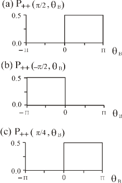
Figure 5: Predicted coincidence curves for the ideal experiment. (a) and (b) illustrate the settings most likely to be chosen in practice, giving the strongest correlations. $\theta_{A}$ is fixed at $\pi/2$ or $-\pi/2$ while $\theta_{B}$ varies. In theory, any value of $\theta_{A}$ between 0 and $\pi$ would give the same curve as (a), any between $-\pi$ and 0 the same as (b). An example is shown in (c), where $\theta_{A}$ is $\pi/4$ but the curve is identical to (a). We do not have rotational invariance: the curve is not a function of $\theta_{B}-\theta_{A}$.

5.2 Fine-tuning the model

Many practical considerations mean that the final local realist prediction will probably not look much like the above step function. It may not even be quite periodic. The main logical difference is that, despite all that has been said so far, the actual variable that is set for the local oscillators is not directly the phase shift but the path length, and, since the frequency is likely to vary slightly from one signal to the next (though always keeping the same as that of the pump laser), the actual phase difference between test and local oscillator beams will depend on the path length difference and on the frequency. In a complete model, therefore, the important parameters will be path length and frequency, with phase derived from these.

If frequency variations are sufficiently large, the situation may approach one of rotational invariance (RI), but it seems on the face of it unlikely that this can be achieved without loss of correlation. If we do have RI, perhaps produced artificially by introducing random phase variations into the OPA pump beam, the model becomes the standard realist one in which the predicted quantum correlation varies linearly with difference in phase settings, but it is more likely that what will be found is curves that are not independent of the choice of individual phase setting. They will be basically the predicted step functions but converted to curves as the result of the addition of noise.

It is essential to know the actual experimental conditions. Several relevant factors can be discovered by careful analysis of the variations in the raw voltages in each homodyne detection system. If noise is low, the presence of the two phase sets, and whether or not they are equally represented, should become apparent.

All this complexity, though, has no bearing on the basic fact of the existence of a hidden variable model and the consequent prediction that the CHSH Bell test will not be violated.

5.3 The role of the “event-ready” detectors

In the quantum-mechanical theory, the expectation of violation of the Bell test all hinges on the production of “non-classical” light. The light directly output from the crystal OPA is assumed to be Gaussian, i.e. it takes the form of pulses of light that have a Gaussian intensity profile and also, as a result of Fourier theory, a Gaussian spectrum. When this is passed through an unbalanced beamsplitter (BS_A or BS_B) and a “single photon” detected by an “event-ready” detector, the theory says that the subtraction of one photon leaves the remaining beam “non-Gaussian”. Although there is mention here of single photons, the theory is concerned with the ensemble properties of the complete beams, not with the individual properties of its constituent pulses.

In the local realist (classical) model considered here, the shapes of the spectra are not relevant except insofar as a narrow band width is desirable for the demonstration of dramatic correlations. The “event-ready detectors” (PD_A and PD_B in Fig. 1) play, instead, the important role of selecting for analysis only the strongest down-converted output pairs, it being assumed that the properties of the transmitted and reflected light at the unbalanced beamsplitters are identical apart from their amplitudes. It is likely that those detected signals that are coincident with each other will be genuine “degenerate” ones, i.e. of exactly equal frequency, quasi-resonant with the pump laser. The unbalanced beamsplitters and the detectors PD_A and PD_B need to be set so that the intensity of the detected part is sufficient to be above the minimum for detection but low enough to ensure that all but the strongest pulses are ignored.

In neither theory are the event-ready detectors really needed in their “Bell test” role of ensuring a fair test (see below), since the homodyne detectors are almost 100% efficient.

6 Validity of the proposed Bell test

Coincidences between the digitised voltage differences will be used in the CHSH Bell test [13, 14], but avoiding the “post-selection” that has, since Aspect’s second experiment [15], become customary. The García-Patrón et al. proposal is to use event-ready detectors, as recommended by Bell himself for use in real experiments [16]. None of the usual loopholes [17] are expected to be applicable:

1. With the use of the event-ready detectors, non-detections are of little concern. The detectors (PD_A and PD_B in Fig. 1) act to define the sample to be analysed, and the fact that they do so quite independently of whether or not any member of the sample is then also detected in coincidence at the homodyne detectors ensures that no bias is introduced here. The estimate of “quantum correlation” to be used in calculating the CHSH test statistic is $E=(N_{++AB}+N_{--AB}-N_{+-AB}-N_{-+AB})/N_{AB}$, where the $N$’s are coincidence counts and the subscripts are self-explanatory. This contrasts with the usual method, in which the denominator used is not $N_{AB}$ but the sum of observed coincidences, $N_{++AB}+N_{--AB}+N_{+-AB}+N_{-+AB}$. The use of the latter can readily be shown to introduce bias unless it can be assumed that the sample of detected pairs is a fair one. That such an assumption fails in some plausible local realist models has been known since 1970 or earlier [14, 18].

2. There is no possibility of synchronisation problems [19], since a pulsed source is used.

3. No “accidentals” will be subtracted [17].

4. The “locality” loophole can be closed by using long paths and a random system for choosing the “detector settings” (local oscillator phase shifts) during the propagation of the signals.

The system is almost certainly not going to be “rotationally invariant” (not all phase differences will be equally likely), but this will not invalidate the Bell test. It may, however, be important in another way. It is likely that high visibilities will be observed in the coincidence curves (i.e. high values of (max – min)/(max + min) in plots of coincidence rate against difference in phase shift), leading to the impression that the Bell test ought to be violated. These visibilities, though, will depend on the absolute values of the individual settings. High ones will be balanced by low, with the net effect that violation does not in fact happen.

7 Validity and significance of negative estimates for Wigner densities

In the quantum mechanical theory discussed in the loophole-free Bell test proposals and in other recent papers [6, 7], part of the evidence that is put forward as indicating that negative Wigner densities are likely to be obtained consists in the observation that, when $\theta$ is varied randomly, the distribution of observed voltage differences shows a double peak (see Fig. 7). There is a tendency to observe roughly equal numbers of + and – results but relatively few near zero. The fact that the relationship depends on the sine of $\theta$ is, however, sufficient to explain why this should be so.

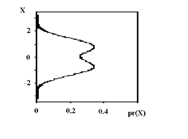
Figure 7: Observed distribution of voltage differences, X, using homodyne detection in an experiment similar to the proposed Bell test and averaging over a large number of applied phase shifts. (Based on Fig. 4a of A. I. Lvovsky et al., Phys. Rev. Lett.  87, 050402 (2001).)

To illustrate, let us consider the following. The sine of an angle is between 0 and 0.5 whenever the angle is between 0 and $\pi/6$. It is between 0.5 and 1.0 when the angle is between $\pi/6$ and $\pi/2$. Since the second range of angles is twice the first yet the range of the values of the sine is the same, it follows that if all angles in the range 0 to $\pi/2$ are selected equally often there will be twice as many sine values seen above 0.5 as below. The same holds when random angles between $\pi/2$ and $\pi$ are chosen, whilst for values between $-\pi$ and 0 we find a symmetrical result for negative values.

When allowance is made for the addition of noise, the production of a distribution such as that of Fig. 7 for the average when angles are sampled uniformly comes as no surprise. Clearly, as the experimenters themselves recognise, the dip is not in itself sufficient to prove the non-classical state of the light. For this, direct measurement of the Wigner density is required, but there is a problem here. No actual direct measurement is possible, so it has to be estimated, and the method proposed is the Radon transformation [20]. It is claimed that in other experiments Wigner densities calculated either by this procedure or by a “more precise maximum-liklihood reconstruction technique” [22] have shown negative regions, but perhaps the methods should be checked for validity?

In any event, as already explained, the natural hidden variable relevant to the proposed experiment is the phase of the individual pulse, not any statistical property of the whole ensemble. Indeed, the use of Wigner density as a substitute for hidden variables was never originally intended and has no theoretical basis. In Bell’s much-quoted paper on the subject (Ch. 21 of ref. [21]), the “hidden variables” remain, as ever, parameters such as position and momentum that are specific to individual particles. The role of the negative Wigner density is merely to provide, in certain rather special circumstances, and alternative test for nonlocality in that, if negative values are found, then real local hidden variables cannot exist.

8 Suggestions for extending the experiment

The basic set-up would seem to present an ideal opportunity for investigation of some key aspects of the quantum and classical models, as well as the operation of the Bell test “detection loophole”.

1. The operation of the detection loophole could be illustrated if, instead of using the digitised difference voltages of the homodyne detectors, the two separate voltages are passed through discriminators. The latter operate by applying a threshold voltage that can be set by the experimenter and counting those pulses that exceed it. These can be used in a conventional CHSH Bell test, i.e. using total observed coincidence count as denominator in the estimated quantum correlations $E$. The model that has been known since Pearle’s time (1970) predicts that, as the threshold voltage used in the discriminators is increased and hence the number of registered events decreased (interpreted in quantum theory as the detection efficiency being decreased), the CHSH test statistic $S$, if calculated using estimates $E=(N_{++}+N_{--}-N_{+-}-N_{-+})/(N_{++}+N_{--}+N_{+-}+N_{-+})$, will increase. If noise levels are low, it may well exceed the Bell limit of 2.

   Such an experiment has, in a sense, already been performed by Babichev et al[22] and yielded the expected results. If it is accepted that their source (two outputs from a beamsplitter) would have been in an entangled state, then their Fig. 4b clearly demonstrates that high detector thresholds (i.e. low detector efficiencies) can lead to violations of the standard form of the CHSH test.

2. The existence of the two phase sets is, in point of fact, well known when OPA’s are operated above threshold [5]. The resonance into one or other of the sets then becomes stable. The fact that that two sets are also responsible for many of the observations below threshold could be further investigated if either the raw voltages or the undigitised difference voltages are analysed. So long as the noise level is low, the existence of the two superposed curves, one for $\alpha=0$ and the other for $\alpha=\pi$, should be apparent. It would be interesting to investigate how the pattern changed as optical path lengths were varied. Breitenbach’s pattern might be hard to reproduce using long path lengths, where exact equality is needed unless the light is monochromatic.

3. Comparison of overall performance: If the primary goal of the experimenter is clearly set out to be the comparison of the performance of the two rival models, rather than merely the conduct of a Bell test, further ideas for modifying the set-up will doubtless emerge when the first experiments have been done. Many of the predictions of the quantum-mechanical model have already appeared in print [3, 4]. The first stage in comparing models should probably be, therefore, to conduct supplementary experiments so as to establish the relevant parameters of the full classical model and hence make equivalent empirical predictions. It is possible, though, that qualitative predictions alone will be sufficient to demonstrate superiority one way or the other.

9 Conclusion

The proposed experiments would, if the “non-classicality” of the light could be demonstrated satisfactorily, provide a definite answer one way or the other regarding the reality of quantum entanglement. They could usefully be extended to include empirical investigations into the operation of the Bell test detection loophole. Perhaps more importantly, though, they present valuable opportunities to compare the performance of the two theories in both their total predictive power and their comprehensibility. Are parameters such as “Wigner density” and “degree of squeezing” really the relevant ones, or would we gain more insight into the situation by talking only of frequencies, phases and intensities? Parameters such as the detection efficiency and the transmittance of the beamsplitters will undoubtedly affect the results, but do they do this in the way the quantum theoretical model suggests? It will take considerably more than just the minimum runs needed for the Bell test if we are to find the answers.

The detailed predictions of the classical model cannot be given until the full facts of the experimental set-up and the performance of the various parts are known, but it gives, in any event, a simple explanation of the double-peaked nature of the distribution of voltage differences. The peaks arise naturally from the way in which homodyne detection works, and the quantum theoretical idea that they are one of the indications of a non-classical beam or of negative Wigner density would not appear to be justifiable. The idea that a classical beam can become non-classical by the act of “subtracting a photon” is, equally, of doubtful validity. The experimental role of the subtraction and detection of part of each beam is to aid the selection for coincidence analysis of those pulses that are likely to be most strongly correlated.

Appendix. Alternative classical derivation of the homodyne detection formula

A derivation is given here that does not involve complex numbers and hence confirms that the equations in the text are ordinary wave equations, not quantum-mechanical “wave functions”.

The relationship between intensity difference and the local oscillator phase can be checked as follows:

Assume the two input beams are

Experimental beam: $E\cos\phi$ , where, as before, $\phi=\omega t$

Local oscillator: $E_{L}\cos(\phi+\theta)$

Then the output beams, assuming a 50-50 beamsplitter and no losses, can be written

Reflected beam:

$$E_{r} = \frac{1}{\sqrt{2}}(E\cos(\phi+\pi/2)+E_{L}\cos(\phi+\theta))$$ (12)

$$= \frac{1}{\sqrt{2}}(-E\sin\phi+E_{L}\cos(\phi+\theta))$$

Transmitted beam:

$$E_{t} = \frac{1}{\sqrt{2}}(E\cos\phi+E_{L}\cos(\phi+\theta+\pi/2))$$ (13)

$$= \frac{1}{\sqrt{2}}(E\cos\phi-E_{L}\sin(\phi+\theta)).$$

Let us define a (constant) angle $\psi$ such that $\tan\psi=E/E_{L}$, making $E\cos\psi=E_{L}\sin\psi$.

Consider the case when $\theta=0$. We have

$$E_{r} = \frac{1}{\sqrt{2}}(E/\sin\psi)(-\sin\psi\sin\phi+\cos\psi\cos\phi)$$ (14)

$$= \frac{1}{\sqrt{2}}(E/\sin\psi)\cos(\psi+\phi),$$

so that amplitude is proportional to $\frac{1}{\sqrt{2}}E/\sin\psi$ and intensity to $\frac{1}{2}E^{2}/\sin^{2}\psi$.

The intensity of the transmitted beam can be found similarly, and turns out to be also proportional to $\frac{1}{2}E^{2}/\sin^{2}\psi$, so that the voltage difference from the homodyne detector is therefore to be zero. Likewise, a zero difference is found for $\theta=\pi$, but other values of $\theta$ produce more interesting results.

For example, for $\theta=\pi/2$ we find

$$E_{r} = \frac{1}{\sqrt{2}}(E/\sin\psi)(-\sin\psi\sin\phi-\cos\psi\sin\phi)$$ (15)

$$= \frac{1}{\sqrt{2}}(E/\sin\psi)\sin\phi(-\sin\psi-\cos\psi),$$

$$E_{t} = \frac{1}{\sqrt{2}}(E/\sin\psi)(\sin\psi\cos\phi-\cos\psi\cos\phi)$$ (16)

$$= \frac{1}{\sqrt{2}}(E/\sin\psi)\cos\phi(\sin\psi-\cos\psi).$$

The difference in intensities is therefore proportional to

Difference $$= \frac{1}{2}(E^{2}/\sin^{2}\psi)[(-\sin\psi-\cos\psi)^{2}$$ (17)

$$- (\sin\psi-\cos\psi)^{2}]$$

$$= \frac{1}{2}(E^{2}/\sin^{2}\psi)4\sin\psi\cos\psi)$$

$$= \frac{1}{2}E^{2}\cos\psi/\sin\psi$$

$$= 2E^{2}E_{L}/E$$

$$= 2EE_{L}.$$

This is consistent with the result obtained by the method in the main text, so it seems safe to accept that as being correct.

References

References

- [1] Bell J S 1964 On the Einstein-Podolsky-Rosen paradox Physics (Long Island City, N.Y.) 1 195
- [2] Bell J S 1971 Introduction to the hidden-variable question, reproduced in Bell J S The Speakable and Unspeakable in Quantum Mechanics (Cambridge University Press 1987)
- [3] García-Patrón R, Fiurácek J, Cerf N J, Wenger J, Tualle-Brouri R, and Grangier Ph 2004 Proposal for a loophole-free Bell test using homodyne detection, Phys. Rev. Lett. 93 130409
- [4] Nha H and Carmichael H J 2004 Proposed test of quantum nonlocality for continuous variables Phys. Rev. Lett. 93 020401
- [5] D Walls and G Milburn 1994 Quantum Optics Springer-Verlag
- [6] Lvovsky A I, Hansen H, Aichele T, Benson O, Mlynek J and Schiller S 2001 Quantum state reconstruction of the single-photon Fock state Phys. Rev. Lett. 87 050402
- [7] Wenger J, Tualle-Brouri R and Grangier Ph 2004 Non-gaussian statistics from individual pulses of squeezed light Phys. Rev. Lett. 92 153601
- [8] Breitenbach G, Müller T, Pereira S F, Poizat J-Ph, Schiller S, Mlynek J 1995 Squeezed vacuum from a monolithic optical parametric oscillator J. Opt. Soc. Am. B 12 2304
- [9] Thompson C H 1999 Rotational invariance, phase relationships and the quantum entanglement illusion (Preprint quant-ph/9912082)
- [10] Breitenbach G and Schiller S 1997 Homodyne tomography of classical and non-classical light J. Mod. Opt. 44 2207–25
- [11] Weihs G, Jennewein T, Simon C, Weinfurter H and Zeilinger A 1998 Violation of Bell’s inequality under strict Einstein locality conditions Phys. Rev. Lett. 81 5039
- [12] Tittel W, Brendel J, Gisin B, Herzog T, Zbinden H and Gisin N 1998 Experimental demonstration of quantum-correlations over more than 10 kilometers Phys. Rev. A 57 3229
- [13] Clauser J F, Horne M A, Shimony A and Holt R A 1969 Proposed experiment to test local hidden-variable theories Phys. Rev. Lett. 23 880
- [14] Thompson C H 1996 The chaotic ball: an intuitive analogy for EPR experiments Found. Phys. Lett. 9 357 (Preprint quant-ph/9611037)
- [15] Aspect A, Grangier Ph and Roger G 1982 Experimental realization of Einstein-Podolsky-Rosen-Bohm gedankenexperiment: a new violation of Bell’s inequalities Phys. Rev. Lett. 49 91
- [16] Clauser J F and Shimony A 1978 Bell’s theorem: experimental tests and implications Rep. Prog. Phys. 41 1881
- [17] Thompson C H 2003 Subtraction of ‘accidentals’ and the validity of Bell tests Galilean Electrodynamics 14 (3) 43–50 (Preprint quant-ph/9903066)
- [18] Pearle P 1970 Hidden-variable example based upon data rejection Phys. Rev. D 2 1418–25
- [19] Fine A 1982 Some local models for correlation experiments Synthese 50 279–94
- [20] Leonhardt U 1997 Measuring the Quantum State of Light (Cambridge University Press, Cambridge)
- [21] Bell J S 1987 Speakable and Unspeakable in Quantum Mechanics (Cambridge University Press, Cambridge)
- [22] Babichev S A, Appel J, and Lvovsky A I 2004 Homodyne tomography characterization and nonlocality of a dual-mode optical qubit Phys. Rev. Lett. 92 193601