The General Quantum Interference Principle and the Duality Computer

Abstract

In this article, we propose a general principle of quantum interference for quantum system, and based on this we propose a new type of computing machine, the duality computer, that may outperform in principle both classical computer and the quantum computer. According to the general principle of quantum interference, the very essence of quantum interference is the interference of the sub-waves of the quantum system itself. A quantum system considered here can be any quantum system: a single microscopic particle, a composite quantum system such as an atom or a molecule, or a loose collection of a few quantum objects such as two independent photons. In the duality computer, the wave of the duality computer is split into several sub-waves and they pass through different routes, where different computing gate operations are performed. These sub-waves are then re-combined to interfere to give the computational results. The quantum computer, however, has only used the particle nature of quantum object. In a duality computer, it may be possible to find a marked item from an unsorted database using only a single query, and all NP-complete problems may have polynomial algorithms. Two proof-of-the-principle designs of the duality computer are presented: the giant molecule scheme and the nonlinear quantum optics scheme. We also proposed thought experiment to check the related fundamental issues, the measurement efficiency of a partial wave function.

I Introduction

The particle and wave nature of microscopic object, is one of the most important aspect of the complementarity principle r1 . A microscopic object possesses both the attribute of a particle and the attribute of a wave, and it displays one attribute at some instances and the other attribute in some other instances. The particle-wave duality of microscopic object is a very mysterious feature of quantum mechanics. This is well stated by Feynman in his physics lecture notes r2

”The quantum interference phenomenon is impossible, absolutely impossible, to explain in any classical way, and it has in it the heart of quantum mechanics”, ”In reality, it contains the only mystery”.

Classically, waves behave quite differently from particles. A wave travels, and splits into many parts when it passes through slits in a wall. When these wave parts meet again, they join together and interfere, constructively or destructively. If we make some changes in one path, say, change its phase, then the interference pattern will change. In contrast, a particle is something that has a definite position in space-time. These seemingly contradicting properties are all exhibited in the very same microscopic object. Taking the double-slits experiment as an example. Suppose an electron starts from a source $S$, ”passes through” a wall with two slits and then hits on a screen. An interference pattern will appear on the screen after sufficient number of particles have been fired. The quotation mark is a reflection of the fact that we do not yet know whether a particle passes through only a single slit, or through both slits simultaneously. What we know is the fact that a particle has passed through the wall and hit on the screen. Any attempt to locate which slit a particle has passed through will eliminate the interference pattern on the screen as shown in the which-way experiment r3 . However without bothering to know which path it passes through, the interference pattern shows up. By varying the phase differences between the two paths, the interference pattern on the screen will change accordingly and in a determined manner.

Interference of light through a double slits was first observed by Young r4 , and it has played a vital role in the acceptance of the wave nature of light. With the development of modern technology, interference of electrons has been obtainedr5 ; r6 ; r7 , and the intensity of the electron can be made so weak that one can observe only a single click on the screen at a given time r7 . A click on the screen is a reflection of the particle nature of electron. Field-theoretic treatment of photon interference was given by Walls in Ref.walls .

Dirac made a famous statement r8 : ” Each photon then interferes only with itself. Interference between two different photons never occurs.” However, sometimes interference of two photons, for instance in Ref.r9 in which two photons, each from the same single photon source but at different instants, do interfere. It seems that Dirac was wrong. We will see that these phenomenon can be naturally explained in the general interference principle of quantum mechanics that we are going to present. From this general principle of quantum interference, interference can occur ont only in a single quantum system, but also occur in composite quantum systems such as electrons in an atom, and even in a quantum system with particles loosely distributed without any binding. This principle will explain different interference phenomena in the quantum world in a unified way.

Physics and computation are closely related. A computing machine is any physical system whose dynamical evolution takes it from one of a set of ”input” states to one of a set of ”output” states. It had been long considered that any computing process can be regarded solely as a mathematical process regardless of the specific computer desginr10 ; r11 . This is true for classical computers and it is explicitly stated in the so-called ”Church-Turing hypothesis”

Every ‘function which would naturally be regarded as computable’ can be computed by the universal Turing machine.

Classical computing process is usually irreversible. Landauer stressed the importance of irreversibility in classical computer and gave the minimum amount of energy a classical computer has to dissipate in erasing or throwing away a bit of informationr12 . But Bennett showed that classical computation can be made reversibler13 . Benioff has constructed a reversible computer using explicitly quantum dynamicsr14 . Feynman pointed out that it was difficult for classical computers to simulate quantum systems efficiently and proposed to simulate quantum systems using quantum computersr15 .

Deutsch replaced the subjective notions such as ”would naturally be regarded as computable” in the Church-Turing hypothesis with objective concepts, and reformulated it into the Church-Turing principler16

Every finitely realizable physical system can be perfectly simulated by a universal model computing machine operating by finite means.

Deutsch further pointed out that the classical universal Turing machine does not satisfy the Church-Turing principle. A universal quantum computer $\cal Q$, however, satisfies this Church-Turing principle.

Thus it began to show that the power of a computer depends closely on the realm of the underlying physics principle. We may conjecture that within a given realm of physics, all computing machines operating with the laws of that realm of physics are equivalent. It is true that all classical computers are equivalent, any classical computer can be perfectly simulated by a universal Turing machine with at most a polynomial slowdown. It is also true that all quantum computers are equivalent r17 . However computers in different realm of physics are not equivalent. For instance a computing machine in the classical physics realm is not equivalent to a computing machine in the quantum mechanics realm. A classical Turing machine can not simulate a quantum system efficiently, whereas a quantum computer can. But among the quantum computers, they are equivalent. The dominance of classical computations has led people to restrict their thinking on the classical computation, and think that computation is solely a mathematical process.

It should be stressed that the nature of a computer should be judged not only by the realm of physics upon which it is operating, but also on the extent to which it has exploited the physics principles of that realm of physics. An electric classical computer working with transistors will be considered the same as a computer working with mechanical means because their underlying physics principles are the same. We will show in this article that the quantum computer uses only the particle nature of quantum system, but not the full power of quantum mechanics. It is superior to classical computer because it has used the superposition principle of quantum mechanics and this has enabled the quantum parallelism in quantum computers. To be exact, the present quantum computer should have been called quantum particle computer, and the type of computer we are proposing here should have been called quantum computer. For historical reasons, we will follow the tradition to call these quantum particle computer as quantum computer and call the computing machine we are proposing as duality computer(DC). Incidentally, the basic information carrier in the duality computer is called duality bit or dubit for short.

When talking about computational complexity, the NP-complete problem is one benchmark. Problems such as the SATISFIABILITY problem r18 requires steps of computation that scales exponentially with the size of the input. In classical computing theory, it is not known if NP=P is true or not. However it is widely anticipated that NP-complete problem is unlikely to have a polynomial solution. In quantum computer, no polynomial algorithm has been found for any NP-complete problem so far. It is also anticipated that $NP$-complete is not equal to $P$ in quantum computers either.

Duality Computer allows more powerful computing operations than what are allowable for a quantum computer. The essential idea of the DC is that the multi-dubits quantum system is treated wholly as a single quantum system. Usually internal degrees such spins are used as dubits. The duality nature of the whole system allows us to divide the quantum wave of the system into multiple parts, or paths, just like an electron passes through a double-slits and divides its wave function into two parts. We can perform different gate operations on different parts of the wave. This is a new type of parallelism, the duality parallelism. Then the different sub-waves are recombined to form the wave of the duality computer. The result of the computation is then obtained by making a measurement. The duality nature of quantum system may offer enormous computing power. The long-term neglect of the duality property in computation may be due mainly to the lack of understanding of the quantum interference of quantum systems with composite components. The quantum duality, or the particle-wave duality, of a single microscopic object is well accepted and understood, but the quantum duality of a composite quantum system is less well understood. This lack of understanding has hindered us from searching more powerful computing machines.

Associated with the quantum duality nature, we also examine other aspects in quantum information processing, for instance the no-cloning theorem r19 . With quantum duality, though we cannot clone an unknown quantum state, we can divide the wave of a quantum state into many sub-waves and each of the sub-wave carries exactly the same unknown (internal) quantum state. Quantum state division operation is a different operation from cloning, and thus it does not contradict the no-cloning theorem.

The article will be organized as follows. In section II, we will present the general quantum interference principle. This includes a reformulation of the quantum interference principle and the generalization to composite quantum systems. In section III we will give a brief review of classical computer and quantum computer. In section IV, we will present a new operation available for duality computing: quantum wave division and quantum wave combination. In section V, we present the major construction of the duality computer. We point out that duality computer provides with us duality parallelism that may enable duality computer to surpass quantum computer. In section VI, we will give, as proof-of-the-principle, two designs of the duality computer: the giant molecule scheme and the nonlinear quantum optics scheme. In section VII, we give duality algorithms for the unsorted database search problem and NP-complete problems. We show that NP-complete = P may be true in duality computer. In section VIII, a concluding remark is given.

II The general quantum interference principle

There are two types of interferences in nature: classical interference and quantum interference. In classical physics, the interference of sound waves and electromagnetic waves are such examples. In these interferences, it is the effect of action that makes the interference. In quantum mechanics, the double-slits interference of electrons is a typical example. It seems that in classical physics, waves from different source can interfere as long as the two waves have a definite phase difference. However, in quantum mechanics, interference takes place when waves of the same quantum object meet in space and time. It is the interference of the existence of the quantum system in quantum interference. Though these two kind of interferences are related, they are different. We restrict ourselves to quantum interference only in this article.

Interference phenomenon has been an important stimulus in the development of quantum mechanics. Not only light, but also particles such as electron and atom exhibit interference when passing through a double-slit. The double-slit experiment is the most popularly known experimental foundations of quantum mechanics. Feynman paid great attention to the experiment, and pointed out the essence of quantum mechanics lies in the double-slits experiment.

Here we first give the general quantum interference principle. This principle is partly a summary of already known results, and partly our generalization.

1. Quantum interference can happen for a quantum system. The quantum system maybe one of the following categories: a single particle such as an electron or fundamental particle, or a composite system with several constituent particles such as an atom or a molecule, or just a collection of particles with no interaction, or binding at all, such as two independent photons. We call the first two categories as a tight quantum system(TQS), and the latter as loose quantum system(LQS).

2. Quantum systems, TQS or LQS, interfere only with themselves through the interference of the waves describing the whole quantum system. If the wave describing the whole quantum system is divided into more than one path and then recombines, quantum interference may occur.

3. Interference of the waves describing the whole quantum system takes place when the waves coincide in the same region in space and in the same period in time. In other word, interference takes place at the same space-time location. The total wave describing the whole quantum system is the sum of all the sub-waves.

4. Interference takes place when the waves are indistinguishable in space and in time. If the system involves identical particles, this has to be taken into account.

5. The wave of the quantum system is characterized by not only the center of mass motion quantum number such as the wave number, but also the internal degree of freedom of the quantum system such as polarization, spin, isospin and other quantum numbers of the constituent particles etc. If the wave function for other degrees of freedom are identical in all the sub-waves, then we can simply consider the center of mass travelling wave functions.

The general principle of quantum interference can be explained from Dirac’s path integral formalism. Suppose the wave function of a quantum system with $n$ constituent particles, loose or bound, is $\psi(x_{1},x_{2},\cdots,x_{n};s_{1},s_{2},\cdots,s_{n},t)$ where $x_{i}$ and $s_{i}$ are the coordinate and the internal degree coordinate of the $i$-th particle, then by generalizing the path integral to include also the internal degree of freedom, we have

$$\psi(x_{1},\cdots,x_{n};s_{1},s_{2},\cdots,s_{n},t)=A\sum_{all\;paths}e^{{i\over\hbar}S[x,s,x^{\prime},s^{\prime}]}\psi(x_{1}^{\prime},\cdots,x_{n};s_{1}^{\prime},s_{2}^{\prime},\cdots,s_{n}^{\prime},t^{\prime}),$$ (1)

where $S[x,s,x^{\prime},s^{\prime}]$ is the action along a path, and $x$, $x^{\prime}$, $s$ and $s^{\prime}$ are short notation for all the $n$ variables respectively. It should be noted that a path here refers to a path in which all the $n$ constituents move from their initial position to their respective final positions. The path integral can be performed in groups separately so that the summation over all paths can be written as a summation over a limited number of distinct paths. For instance, in a one-dimensional free particle case, though there is only a single path from position A to another position B, the electron can still assume numerous kinds of motion along that path: at each point in the one-dimensional space, an electron can have different velocity. After performing the summation over the different paths, we are left with a free particle wave function. For a double-slits, such a treatment leaves us two distinct routes, each being a free particle wave function, one from the upper path and one from the lower path.

Sometimes we also refer the wave as the probability amplitude according to its interpretation in quantum mechanics. Let’ study these five criteria for quantum interference one by one. The first criterion is a generalization of Dirac’s statement into systems with more than one microscopic particles. There are experimental evidence. There is no doubt that a photon or an electron can only interact with itself. The quantum interference of a composite quantum system have also been experimentally demonstrated by the Vienna group using giant molecules and biological large molecules r31 . The interference of TQS is generally accepted, and one usually has no difficulty in comprehend it.

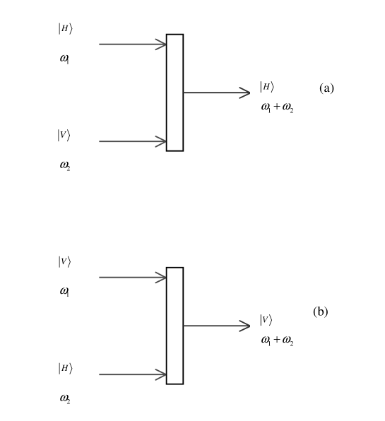
Figure 7: Type II up-conversion. (a) Case 1 of type II SFG; (b) Case 2 of type II SFG.

The quantum interference of two-photon that are generated from type-II down conversion simultaneously can occur r21 . The two photons produced in the type-II down conversion was suggested by Shih as a ”two-photon” particle, which should be treated at the same footing as a composite particle though they are separated in space. Other two photon interference phenomenon can also be explained in the ”two-photon” picture zhangsun . A simplified illustration is shown in Fig. 7 of Ref.r21 . In the middle is a nonlinear crystal. Due to type-II down conversion, two photons are generated simultaneously. The frequency of these two photons are not necessarily equal. Here One photon, is moving to the left, and after passing through a double-slits screen is detected by detector D₁. The other photon is moving to the right and is detected by detector D₂ after passing through a single slit in screen S₂. When observing the coincidence measurements of the two detectors, interference pattern is observed in the plot of the coincidence number versus the vertical position of detector D₂. This interference phenomenon can be understood in the following way. The two photons can be generated in several different possible positions in the nonlinear crystal. For the two photons measured by the coincidence measurement, they can be generated in a position in the upper part of the crystal, or a position in the lower part of the crystal. Thus two waves, or sub-waves to be more exact, that describe the same two-photon system exist. After generation they travel to the left and right respectively either through the upper path, or through the lower path. At the detectors, the two sub-waves from these two paths are indistinguishable at the detectors, that is the detectors can not distinguish either the two photons detected are generated in a position at the upper part of the crystal and travel leftwards and rightwards towards the them respectively or from a position in the lower part of the crystal and then travel to them through the lower path. Hence they combine and produce interference. It is really the interference of the same quantum system, the system with two photons generated in the type-II down conversion. There is no interference between the left photon and the right photon. These two photons is a generalized composite particle system just like an atom or a molecule. Different from a usual composite particle such as an atom, the constituent particles such as the two photons are not combined together, and the distance between them is changing. Whereas in an atom, the constituent particles are combined together and are located in the same area in space.

It is also interesting to point out that the interference pattern can also be observed if a delayed measurement is performed in the right detector D₂. D₂ can be placed in a position that is farther away from the crystal than that between D₁ and the crystal. Hence the left photon is detected first, and the right photon is detected later. There is no interference in the plot of the counts in detector D₁ versus the vertical position. However, if the coincidence of the two detectors is made, with suitably chosen delay time according to the geometry of the experimental setup, interference pattern is seen clearlyr21 .

The second criterion is a concretization of Dirac’s statement for a single photon in terms of wave functions and a generalization to quantum system with multiple particles. For a single quantum particle such as a photon, the interference takes place only by itself through its wave functions or amplitude probabilities. For instance, when it passes through a double-slits, the wave function of a photon is divided into two parts, and they then recombine at the spot on the detection screen. The wave function of the photon is a function of both the position, and the photon polarization. Suppose the two slits in the screen are identical in every aspects, then the quantum wave function $|\psi\rangle|\chi\rangle$ will be split into two parts with equal coefficients,

$${1\over 2}|\psi_{u}(t)\rangle|\chi\rangle={1\over 2}|\psi_{u}(t),\chi\rangle,$$

in the upper path and

$${1\over 2}|\psi_{d}(t)\rangle|\chi\rangle={1\over 2}|\psi_{d}(t),\chi\rangle$$

in the lower path where the coefficients have been renormalized to give the right intensity. $|\chi\rangle$ represents the internal wave function, polarization wave function, of the photon. The internal wave function has the same form in the upper and lower paths because we have assumed that the two paths do not affect the internal wave function. This degree of freedom is usually ignored in double-slits experiment with photons. In the neutron interference experiment however, this degree of freedom has been taken into consideration explicitlyr22 .

The difference between the two kinds of complex systems, the TQS and LQS, is that for the TQS such as a giant molecule, the whole system as a whole moves like a single particle, for instance when passing through a double-slits, there are two possibilities, either from the upper slit or from the lower slit, while for a LQS with two independent photons, they do not have this combined behavior while in motion, and there will be four possibilities when the two photons pass through a double-slits, either both pass through the upper slit, or the lower slit, or photon A passes through the upper and the photon B passes through the lower slit, or the photon A passes through the lower slit and the photon B passes through the upper slit. As long as they satisfy the conditions for interference, quantum interference will take place. For the TQS case, one can still observe an interference pattern just like that for an electron passing through a double-splits. However, for the LQS such as two independent photons generated simultaneously, interference can only be observed with two detectors and with coincidence, and the interference pattern is the result of four sub-waves.

It is interesting to generalize the double-slits into multiple-slits. When there are $d$-slits on the wall, a quantum wave passing through the wall will be divided into $d$ sub-waves. We assume that these slits are identical, then at positions near the slits just after the wall, each sub-wave is ${1\over d}|\psi\rangle$ apart from a phase difference in the coordinate wave function and $|\psi\rangle$ includes both the spatial wave function and the internal wave function. Here again a renormalization of the coefficients has been taken so that if the $d$ sub-waves recombine with the same phase at the detector, they will add up constructively to give $|\psi\rangle$. For instance a three-slits wall will divide a wave into 3 parts, each with $1/3|\psi\rangle_{i}$ where the subscript $i$ indicates the path number. However this information should not be available at the detector, otherwise the interference pattern will disappear. If one of the slits, say slit 1 is distinguishable from the other two slits, the sub-wave on path 1 becomes $\sqrt{1/3}|\psi\rangle_{1}$ whereas the other two sub-waves becomes $1/2\sqrt{2/3}|\psi\rangle_{2}$ and $1/2\sqrt{2/3}|\psi\rangle_{3}$ respectively. Then on the screen, we should have a combined result of the incoherent summation of a single-slit electron pattern having 1/3 of the total intensity together with an interference result from slit 2 and slit 3 having 2/3 of the total intensity. This can be realized if we let the spin polarization at slit 1 in spin up state and at slits 2 and 3 in spin down state. If we have all the path information, then there will be no interference at all, just like what happens in the which-way experiment.

Criterion 3 is the necessary condition for interference, just like that for classical waves. A wave train has a limited length, which maybe different for different systems. For instance, for the down-conversion produced photonsr23 , the wave train is about 16$\mu m$ long and has a time span of about 100$fs$. Usually interference will be the strongest if all the waves coincide closely in space and synchronize in time. If two sub-waves do not overlap, then there will be no interference.

Criterion 4 further specifies the condition for interference. If the internal states are different, they will not interfere even though they coincide in space and time. It is also a special case of criterion 5 in which all other attributes of the sub-waves are identical. The sub-waves become indistinguishable when all other degrees of freedom become identical and the only difference between the different sub-waves at the coalescing region are the amplitudes and the phases of the center of mass motion (or called the spatial mode). If the other degrees of freedom are not identical between the different waves, the overlapping between the different waves will decrease and hence produces less or no interference. For instance, in a double-slits experiment, suppose the sub-wave from the upper slit and the sub-wave from the lower path are made to have different, orthogonal internal states, ${1/\sqrt{2}}|\psi_{u},\chi_{1}\rangle$ and ${1/\sqrt{2}}|\psi_{d},\chi_{2}\rangle$. When they join together the total wave become $|\psi_{t}\rangle={1/\sqrt{2}}|\psi,\chi_{1}\rangle+{1/\sqrt{2}}|\psi,\chi_{2}\rangle$. Then the probability to find a particle is

$$\langle\psi_{t}|\psi_{t}\rangle = {1\over 2}\langle\psi,\chi_{1}|\psi,\chi_{1}\rangle+{1\over 2}\langle\psi,\chi_{2}|\psi,\chi_{2}\rangle+{1\over 2}\langle\psi,\chi_{1}|\psi,\chi_{2}\rangle+{1\over 2}\langle\psi,\chi_{2}|\psi,\chi_{1}\rangle$$ (2)

$$= {1\over 2}\langle\psi,\chi_{1}|\psi,\chi_{1}\rangle+{1\over 2}\langle\psi,\chi_{2}|\psi,\chi_{2}\rangle,$$

where $\langle\chi_{1}|\chi_{2}\rangle=0.$

A special case is the identical particle system. In the experiment in Ref.r9 , two photons emitted at different instants from a single quantum well are guided into the two ports of a beam splitter. Then the two cases of one photon being reflected and one photon being transmitted are indistinguishable. The two photons are identical photons, though they are generated in different instants. If one could make the two photons to have different frequency, then interference would have disappeared. The interference of light from two independent, but synchronized lasers, can be understood in this view. For instance, the light was made so weak that at any given instant with high probability there was only a single photon in the experimental set-upindependent . Because a photon produced from a laser is indistinguishable from a photon from the other laser. These two waves can superpose at the detector to interfere. It is somehow similar to the two-photon interference experiment where the two photons can either be produced in the upper part or the lower part of the crystal.

Criterion 5 has been largely neglected before. In addition to the space attribute, a quantum system also has other degrees of freedom such as spin for electron, the polarization for photon, the states of the electrons, nuclei of the atoms inside a fullerene molecule. When a quantum system passes through two identical slits, the wave function in fact has been split into

$${1\over 2}|\psi_{u},\chi\rangle,$$ (3)

for the upper slit, and

$${1\over 2}|\psi_{d},\chi\rangle,$$ (4)

for the lower slit. Here the internal states are identical. They can become different if we apply different operations on the internal degrees of freedom for the different parts. In fact, the disappearance of interference in the which-way experiment is because the internal state of the different paths are different where the internal states in the different paths are in fact orthogonal.

Conversely, if we manage to make the spatial part of all the sub-waves to have the same phase, when they combine, the spatial part becomes a common factor and the summation is carried out only in the internal part of the sub-waves. Then we will see interference patterns arising from the internal degree of freedom.

In general, the total wave of a quantum system is the sum of all the sub-waves from different paths, if the sub-waves from different path are not orthogonal, then interference will occur, whether partially or completely.

III Classical Computers and Quantum Computers

Though logic does not limit the set of computable functions of a computing machine, physics does. In classical computer, all possible computing functions are restricted by the set of computable functions of the universal Turing machine. This limitation is not due to mankind’s wisdom in computer design, nor by the ingenuity in constructing models for computation, but is universal. This limitation can only be broken by the use of a different underlying physics, namely the kinds of operations that are allowable in the computing process. Generally, low-level physics is some approximation of a more advanced physics. For instance, Newtonian mechanics can be regarded as the low speed approximation of Einstein’s relativistic mechanics, and classical physics is the macroscopic limit of quantum mechanics. Computing machines operating with an advanced physics principle will cover the computing machines operating with a less advanced physics in terms of computing power. In a universal quantum computer, quantum parallelism exists, and it adds additional computing power over classical computer. For instance, Shor’s algorithm can factorize a large integer in polynomial timer24 . Grover’s algorithm can find a marked item from an unsorted database with $O(\sqrt{N})$ stepsr25 ; r26 , whereas $O(N)$ steps have to be searched on a classical computer. The types of calculations available for a quantum computer is also restricted by the physics principle, for the unsorted database search problem Grover’s algorithm is the fastest that a quantum computer can dor27 .

Typically, a quantum computer consists of two components, a finite processor and an infinite memory taper16 . The computation is performed in steps of fixed time duration $T$, and during each step the processor only interacts with a finite part of the memory, and the rest of the memory remains static. The state of $\cal Q$ is a unit vector in the space $\cal H$ spanned by the simultaneous eigenvectors

$$|x;\hat{n};\hat{m}\rangle\equiv|x;n_{0},n_{1},\ldots,n_{M-1};\ldots,m_{-1},m_{o},m_{1},\ldots\rangle,$$ (5)

where $x$ is the ”address” number of the currently scanned tape location. $\hat{n}$ is the state of the processor and $\hat{m}$ is the tape eigenvectors. This is the computational basis states. The dynamics of $\cal Q$ is represented by a constant unitary operator $U$ on $\cal H$. $U$ specifies the evolution of any state $|\psi(t)\rangle\in\cal H$. The effect of $U$ on $\cal H$ can be represented by

$$\langle x^{\prime};\hat{n}^{\prime};\hat{m}^{\prime}|U|x;\hat{n};\hat{m}\rangle=\left[\delta^{x+1}_{x^{\prime}}U^{+}(\hat{n}^{\prime},m^{\prime}_{x}|\hat{n},m_{x})+\delta^{x-1}_{x^{\prime}}U^{-}(\hat{n}^{\prime},m^{\prime}_{x}|\hat{n},m_{x})\right]\Pi_{y\neq x}\delta^{m_{y}}_{m_{y}},$$ (6)

which indicates that the scanning head can move one step to the left or to the right each time. $\hat{n}^{\prime}$ and $\hat{n}$ are the labellings of the processor’s internal state, and $m_{x}^{\prime}$ and $m_{x}$ are the labellings of the tape that have been involved in the interaction with the processor after and before the tape head movement.

Two models of quantum computer exist. The universal quantum Turing machine resembles straightforwardly the classical universal Turing machiner16 . Similar to the von Neunman’s logic circuit network model of classical computer, there is the quantum circuit network modelr17 . Yao has showed that the two models of quantum computer are equivalentr17 :

Let $\cal M$ be a quantum Turing machine and $n$, $t$ be positive integers. There exists a quantum Boolean circuit $K$ of size $poly(n,t)$ that $(n,t)$-simulates $\cal M$.

A quantum Boolean circuit $K$ with $n$ input variables is said to $(n,t)$-simulate a quantum Turing machine $\cal M$, if the family of probability distributions $P_{\tilde{x}}$, $\tilde{x}\in\{0,1\}^{n}$ generated by $K$ is identical to the distribution of the configuration of $\cal M$ after $t$ steps with $\tilde{x}$ as input. Yao also proved that a universal quantum Turing machine can simulate any given quantum Turing machine with only a polynomial slow-down, and hence all quantum Turing machines are computationally equivalent.

Quantum Turing machine model is attractive to computer scientists. To physicists, the quantum computational network model is more attractive. In quantum computational network, there are quantum gates, sources, sinks and unit wires. A quantum computing process can be viewed as a certain number of qubits prepared in some initial states, passing through a series of quantum gates and finally be measured. In a quantum computational network, the evolution is from left to right. All quantum gate operations are unitary. Unitarity is a requirement in quantum mechanics that all observables are hermitian, especially the hamiltonian of the system. A quantum gate operation can be seen as the controlled evolution of the quantum system consisting of all the qubits. Suppose that the initial state of a quantum computer is $|\psi_{i}\rangle$. After the action of a sequence of quantum gate operations, the state of the quantum computer becomes $|\psi_{f}\rangle$, and the process can be written as

$$|\psi_{f}\rangle=G_{n}G_{n-1}\ldots G_{1}|\psi_{i}\rangle,$$ (7)

where each $G_{i}$ is a gate operation. A gate operation can be an arbitrary unitary operation on the Hilbert space $\cal H$ span by the $2^{n}$-basis states of the $n$ qubits system. After the completion of the gate operation a projective measurement on the quantum computer is made to read out the result. Certain outcome will appear probabilistically.

The most distinct feature of quantum computation is the quantum parallelism. When acting on the superposition of all the computational basis states with a unitary operation effecting a function $f$, $U_{f}$,

$$U_{f}{1\over\sqrt{N}}\sum_{i=0}^{N-1}|i\rangle|0\rangle={1\over\sqrt{N}}\sum_{i=0}^{N-1}|i\rangle|f(i)\rangle,$$ (8)

the quantum computer calculates all the function values of the function $f$ and puts them in the second register. The right-hand-side of eq. (8) contains the result of an arbitrarily large number $N$ computations of the function $f$, which would require a classical computer $N$ number of computations to complete.

Unitarity of operations in quantum computer has set very stringent restrictions on the computing power of the quantum computer. For instance, using the unitarity property, it has been shown that Grover’s algorithm is optimal for quantum computersr27 in finding a marked state from an unsorted database. Though great computational powers have been delivered by the quantum computer, there are still limitations. There have been no polynomial solutions to any NP-complete problems so far. In some problems, the quantum computer offers no speedup at all. It seems that the quantum computer maybe efficient in simulating local quantum systems. But it is very restricted in solving general mathematical hard problems. For example, the Grover algorithm only achieves a square-root speedup, and it still scales exponentially with the input size.

Can we do better than quantum computer in computations? The power of a computing machine is ultimately determined by the underlying physics principle. If we restrict ourselves to only classical physics, then we can only have the computing power of a classical Turing machine. Though there have been many efforts to find polynomially quantum algorithms for NP-complete problems, it seems difficult. We can do better if we go out of the underlying physics realm of quantum computer.

IV quantum wave divider and quantum wave combiner in duality computer

We use quantum optics to illustrate some basic element in a quantum duality information processer. We use the two polarization states of a photon as the two quantum levels of a dubit. A dubit possesses the duality nature of quantum mechanics and thus can allow more operations than a qubit where it is a special case of a dubit when a dubit takes on only a single path. We denote the horizontal polarization state as $|0\rangle$ and the vertical polarization state as $|1\rangle$. The photon polarization can be rotated through a polarization modulator, for example in a Pockel cell. We denote the effect of such a polarization modulator as $U_{\theta}$, mathematically, it can be expressed as

$$U_{\theta}|0\rangle =\cos\theta|0\rangle+\sin\theta|1\rangle,$$

$$U_{\theta}|1\rangle =-\sin\theta|0\rangle+\cos\theta|1\rangle.$$ (9)

A phase modulator can add a given phase to a photon state. It is usually a variable wave-plate. Its effect can be written as

$$P_{\lambda}|\psi\rangle=e^{i\lambda}|\psi\rangle.$$ (10)

Here the effect is written out as if the dubit has only a single path. When a dubit has two paths, the effects of such devices are only on the specific sub-wave along a path.

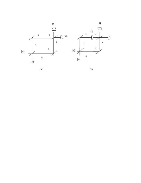
Figure 1: A Mach-Zehnder Interferometer (a) without phase modulator, and with a phase modulator (b).

A beamsplitter is a common optics component. There are two kinds of beamsplitters: the ordinary beamsplitter or beamsplitter for short, and the polarization beamsplitter. A beamsplitter is insensitive to the photon polarization states, whereas the polarization beamsplitter is sensitive to the polarization of the photon. A beamsplitter with two input modes $a$ and $b$ and two output modes $c$ and $d$ is shown in Fig.1a. When a photon enters a beamsplitter from one port, depending on which side the photon hits the beamsplitter, it transforms the photon state into

$$|a\rangle \longrightarrow{i}\cos\theta|c\rangle+\sin\theta|d\rangle,$$

$$|b\rangle \longrightarrow\sin\theta|c\rangle+i\cos\theta|d\rangle.$$ (11)

For a 50-50 beamsplitter, $\theta=\pi/4$. Then its transformation is

$$|a\rangle \longrightarrow{i\over\sqrt{2}}|c\rangle+{1\over\sqrt{2}}|d\rangle,$$

$$|b\rangle \longrightarrow{1\over\sqrt{2}}|c\rangle+{1\over\sqrt{2}}|d\rangle.$$ (12)

It means that a 50-50 beamsplitter reflects the photon and transmits the photon with half probability respectively. The reflected part has additionally a half $\pi$ phase factor: $e^{i\pi\over 2}=i$. Suppose a photon enters a beamsplitter from input mode $a$, after the beamsplitter, the state of the photon becomes

$${i\over\sqrt{2}}|c\rangle+{1\over\sqrt{2}}|d\rangle.$$

This resembles the case of a double-slits in which the path information is known: we know the information of which path the photon will take if we place a detector far away from the beamsplitter on each side of the beamsplitter. In this case, the two sub-waves of the output ports do not recombine so no interference occurs between the two output mode of the beamsplitter. To resemble a double-slits interference, we have to eliminate the path information, and we need another beamsplitter arranged in a Mach-Zehnder interferometer as shown in Fig 1b, then at the detector $D_{f}$ interference of the sub-waves takes place. The state of the photon goes the following changes leading to the detector

$$|a\rangle\longrightarrow BS_{1}\begin{array}[]{ccccc}\nearrow&i\sqrt{1\over 2}|c\rangle\rightarrow&M_{1}\rightarrow&i\sqrt{1\over 2}|c\rangle&\searrow\\ \searrow&\sqrt{1\over 2}|d\rangle\rightarrow&M_{2}\rightarrow&\sqrt{1\over 2}|d\rangle&\nearrow\end{array}BS_{2}\rightarrow\left(i\sqrt{1\over 2}\sqrt{1\over 2}+\sqrt{1\over 2}i\sqrt{1\over 2}\right)|f\rangle=i|f\rangle.$$ (15)

Here the two sub-waves interfere constructively at the detector $D_{f}$. It is clear, the sub-waves from the two paths each contributes $1/2$ to the total wave at the detector. To simulate the double-slits experiment, we can vary the phase factor in one of the arms as shown in Fig.1b, then the wave function experiences the following change

$$|a\rangle\longrightarrow BS_{1}\begin{array}[]{cccccc}\nearrow&i\sqrt{1\over 2}|c\rangle\rightarrow&M_{1}\rightarrow P_{\lambda}\rightarrow&ie^{i\lambda}\sqrt{1\over 2}|c\rangle&\searrow\\ \searrow&\sqrt{1\over 2}|d\rangle\rightarrow&M_{2}\longrightarrow&\sqrt{1\over 2}|d\rangle&\nearrow\end{array}BS_{2}\rightarrow i\left(1+e^{i\lambda}\over 2\right)|f\rangle+\left({1-e^{i\lambda}\over 2}\right)|e\rangle.$$ (18)

As $\lambda$ changes from 0 to $\pi$ and $2\pi$, we have at the detector a maximum, then a minimum and then another maximum, which resembles perfectly a double-slits experiment. In detector $D_{e}$, we see a complementary result. In the following we will use interchangeably the double-slits and the Mach-Zehnder interferometer to describe the physical realization schemes of the duality computer.

A quantum wave divider is a device that divide a quantum wave into several sub-waves, and each sub-wave possesses the same internal quantum state as that of the input wave function. Let a particle passing through a double-slits, there are two paths: one from the upper slit and the other from the lower path. Sub-waves from these two paths will interfere at the screen where they become indistinguishable. In addition to the path information, a particle has also internal degrees of freedom, for instance a photon has polarization and an electron has spin. During the process of the particle passing through the double-slits, the internal degrees of freedom remains the same, say at $(a|0\rangle+b|1\rangle)$, the only thing that is different is the spatial information. Hence the upper wave maybe written as

$$|\phi_{u}\rangle={1\over 2}(a|0\rangle+b|1\rangle)|\psi_{u}\rangle,$$ (19)

whereas the low-path wave function is

$$|\phi_{d}\rangle={1\over 2}(a|0\rangle+b|1\rangle)|\psi_{d}\rangle,$$ (20)

where $|\psi_{u}\rangle$ and $|\psi_{d}\rangle$ are the spatial wave function for the upper and lower path respectively. It is interesting to note that here we have two sub-waves that has exactly the same internal states. Their only difference is in the spatial mode. It is not a clone of the state of one particle onto another particle, it is a division of state of the same particle. When there are multi-slits in the wall, the quantum wave of the particle will be divided into multiple sub-waves. Again each sub-wave has the same internal states.

Now we generalize the above discussion to a complicated quantum system such as a giant molecule. Suppose a giant molecule has $n$ spin-1/2 nuclear spins. Each nuclear spin is used as dubit. Let the states of these $n$ nuclear spins be denoted $|\chi_{n}\rangle$ . When the giant molecule passes through a double-slit, the wave is divided into two sub-waves, $|\psi_{u}\rangle|\chi_{n}\rangle$ and $|\psi_{d}\rangle|\chi_{n}\rangle$. The internal state of these sub-waves are identical. This is a special design of a quantum wave divider (QWD). We can generally assume that for a general quantum system, there exists an QWD operation that divides the total quantum wave into several sub-waves in different spatial modes but with identical internal wave function. This is possible when we use the quantum duality property. This important ingredient is missing in a quantum computer.

A quantum wave combiner(QWC) is a device that does the reverse effect of a quantum wave divider: it combines the sub-waves of a quantum system into a single wave. For instance two sub-waves from a double-slits combine at the screen and interference occurs. In general we assume such a device can be built for a given quantum system. QWD and QWC are crucial for the duality computer. When a quantum system is not measured, it behaves like a wave, can be divided or combined, and when it is measured it behaves like a particle. In this article we represent the QWD and QWC using symbols as shown in Fig.2 where a quantum system with dubits are drawn.

Before going to a general DC, we demonstrate the use of a single dubit to perform duality computing. We write out here only the internal state of the quantum system which is the state of the dubit. After the QWD, the state of a dubit $a|0\rangle+b|1\rangle$ is divided into two sub-waves passing in two different paths. On each path, we perform some gate operation, which is composed of a series of unitary gate operations, on the dubit. For instance we can perform only a unitary operation $U$ on the upper path, and the upper sub-wave becomes

$$|\psi^{\prime}_{u}\rangle={1\over 2}U(a|0\rangle+b|1\rangle)={1\over 2}(a^{\prime}|0\rangle_{u}+b^{\prime}|1\rangle),$$ (21)

where we have omitted the spatial part of the sub-wave. At the screen the two sub-waves combine to form the wave

$$|\psi\rangle_{f}={a+a^{\prime}\over 2}|0\rangle+{b+b^{\prime}\over 2}|1\rangle.$$ (22)

Here again the spatial wave function is not written out explicitly. It is always possible to arrange the two paths to have the same lengths so that the phase difference between the two paths are multiples of $2\pi$, namely at the QWC the spatial wave functions from the two paths are identical and is a common factor. After measurement, the result is then read out.

Wootters and Zurek have shown that quantum state can not be clonedr19 . In a cloning process, it is to clone the quantum state of one particle onto another different particle. In this splitting of quantum state in a double-slits, it is self division of the quantum state on different spatial degrees freedom, however the whole wave, both the internal wave and the spatial wave together represent the state of the particle.

V The Duality Computer and duality parallelism

A duality computing machine uses the particle-wave duality property of quantum mechanics for computation. In a duality computer, the wave functions of the multi-dubit duality computer can split into two paths. The two paths have the same spatial length, that is, when a duality computer passes through these two paths and recombine its wave function at the QWC, the spatial mode of the two sub-waves are in phase. If there is only one path, then the duality computer reduces to quantum computer which is presently under extensive study worldwide.

Two components are crucial in duality computer: the QWD and the QWC, as have been introduced in previous section. For a single particle quantum system, a QWD is just a beamsplitter or a double-slits. When a photon passes it, there are 50% probability to be reflected and 50% probability to be transmitted through the beamsplitter. But for a multi-photon quantum system, a QWD is much more complicated, and I shall give a specific implementation of a QWD in later section. After the QWD, the wave splits into two sub-waves in different paths. We can perform gate operations on each sub-wave separately. Then the two sub-waves are combined in a QWC so that interference may take place. The result of the calculation can be read out by a final measurement. For a single quantum particle, a QWC is just the screen in a double-slits experiment. However for multi-photon system, the construction of QWC is complicated and examples will be given in later section.

There are several issues I should like to emphasize.

First, on a single path, the gate operations is assumed unitary. Unitary operation is performed on a path in a duality computer just as if we were operating on the whole quantum system. Dubit is on constant motion, because particle wave duality is reflected when the quantum system is moving. For a quantum computer, it is usually located at some area in space so that when one makes a measurement he/she always find the quantum computer there. Though there are some proposed physical realizations using flying qubits such as photons, it is essentially a quantum particle computer as it is equivalent to the static quantum computer realization. Therefore some modification on the way to perform gate operation should be made. We will discuss this in the giant molecule scheme in the next section. Though the operation in each path is unitary, the operation on the whole duality computer is not. This is not surprising for we are considering only a part of the space. For instance in the Mach-Zehnder interferometer setup, if we just look at one outport we sometimes do not observe a photon though a photon is injected into the interferometer. However if we look at both detectors we always observe one when one photon is injected. This is fundamentally different from a quantum computer where every gate operation must be unitary, and the whole quantum system takes only a single path. Thus it is apparent that when there is only a single path in a duality computer, it reduces to a quantum computer. The relationship between duality computer, quantum computer and classical computer can be seen as follows: when a duality computer is allowed to compute with only a single path, duality computer reduces to a quantum computer. There is no duality in quantum computer, but superposition and entanglement are still available in quantum computer. If we allow a quantum computer to calculate using only the computational basis states, a quantum computer reduces to a classical computer where neither superposition nor entanglement are present.

Secondly, besides the QWD and QWC, other gate operations are needed to implement the unitary operations in each individual path. It has been proven that a set of basic gate operations is sufficient to construct any unitary operationr28 . It is known that single bit rotation gate and two qubit control not(CNOT) gate form a set of universal gater30 . This universal set of gate can also be employed in duality computer. Of course other sets of universal quantum gate operations could also be adopted. As an example a universal set of duality computing gate operations can be: the QWD, QWC, 2-dubit CNOT and single bit rotations.

Thus the computing process in a quantum duality computer can be illustrated as follows

$$|\psi,\phi\rangle\longrightarrow{\rm QWD}\begin{array}[]{lllll}\nearrow&p_{1}|\psi,\phi_{1}\rangle&\longrightarrow&p_{1}U_{1}|\psi,\phi_{1}\rangle&\searrow\\ \searrow&p_{2}|\psi,\phi_{2}\rangle&\longrightarrow&p_{2}U_{2}|\psi,\phi_{2}\rangle&\nearrow\end{array}{\rm{QWS}}\rightarrow(p_{1}U_{1}+p_{2}U_{2})|\psi,\phi\rangle,$$ (25)

where $p_{1}\geq 0$, $p_{2}\geq 0$ and $p_{1}+p_{2}=1$, $\psi$, the first part in the state ket is the internal wave function which is the state of the duality computer, $\phi$ is the spatial wave function. The gate operation $U_{1}$ and $U_{2}$ are both unitary, and they act on the internal wave function. They themselves are composed of basic one bit and two bit gate operations. However, when they recombine at the QWS, which leads to

$$p_{1}U_{1}|\psi,\phi_{1}\rangle+p_{2}U_{2}|\psi,\phi_{2}\rangle\rightarrow({p_{1}U_{1}+p_{2}U_{2}})|\psi,\phi\rangle,$$ (26)

where the subscript in $|\phi_{i}\rangle$ has been dropped because the spatial part of the two sub-waves become identical at the QWC. The total operation is not unitary. For instance for a symmetric QWD, $p_{1}=p_{2}=1/2$,

$$\left(U_{1}+U_{2}\over 2\right)^{\dagger}\left(U_{1}+U_{2}\over 2\right) = {1\over 4}\left(U_{1}U_{1}^{\dagger}+U_{2}U_{2}^{\dagger}+U_{1}U_{2}^{\dagger}+U_{2}U_{1}^{\dagger}\right)$$ (27)

$$= {1\over 4}\left(2I+U_{1}U_{2}^{\dagger}+U_{2}U_{1}^{\dagger}\right)\neq I.$$

Eqs. (25) or (26) show that the duality computer has a more powerful parallelism, the duality parallelism. One can perform different operations to the sub-waves in different paths. While in quantum computer, this parallelism is absent. Thus in duality computer, both the products of unitary operations and the linear superpositions of unitary operations are permissible. This contrasts to the quantum computer where only the product of unitary operations are allowed. Since every $2^{n}\times 2^{n}$ matrix can be written as linear combination of unitary matrices, therefore a duality computer can implement any type of operations in the Hilbert space.

This is the simplistic duality computer model. Instead of dividing the quantum wave into two sub-waves, we can divide it into multiple sub-waves. Furthermore, the division can also be done for the sub-wave in each path to produce sub-sub-waves. In theory, this division can be performed at an arbitrary level. This further division may provide convenience and additional benefit in solving a specific problem. It will be an interesting investigation to study the computational complexities of the duality computer. We can use the number of paths in a QWD and the levels of use of QWD to describe the structure of a duality computer. For instance we call the DC described in Eq.(25) as a 1-level 2-paths duality computer. If the divider has 3 outputs where another QWD is used at path 2 in Eq.(25), then the duality computer will be a called a 2 level 3-paths duality computer.

VI Implementations of DC: the giant molecule scheme and the nonlinear quantum optics scheme

I give two physical realizations of the duality computer. One is the giant molecule scheme, and the other is the nonlinear quantum optics realization.

VI.1 The Giant Molecule Duality Computer

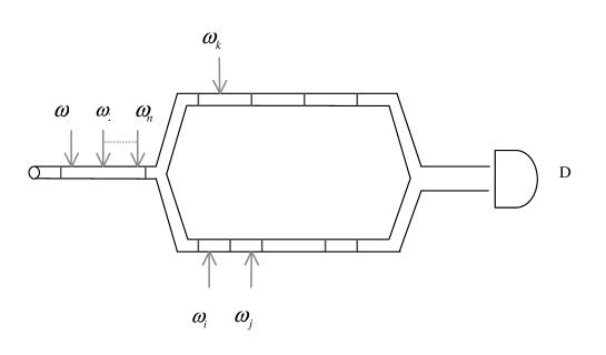
Figure 3: A Duality Computer with Nuclear Spins from a Giant Molecule.

A A spin-1/2 nuclear spin has two quantum state. $n$ nuclear spins might act as an $n$-dubit duality computer. However if we let these $n$ dubits to pass through a double-slits device, there are many configurations. Say we have two dubits, then there will be 4 possibilities for the two particles to be measured at a given place on the screen: 1) both pass through upper slits; 2) both pass the lower slits; 3)particle A passes through upper and particle B passes through lower slit; 4) particle A passes through lower slit and particle B passes through the upper slit. What we need for the duality computation are the two paths that both particles go through the upper slit or the lower slit. Hence it is not workable if we simply use $n$ number of dubits. We need something that bounds all the $n$ dubits so that they will pass through the upper slit as a whole or pass through the lower slit as a whole. This is the function of QWD. The giant molecule is a good candidate quantum system for such purpose. It has been demonstrated that giant molecules exhibit quantum interferencer31 even though the internal states are complicated. Here we use a hypothetical molecule which contains many spin-1/2 nuclear spins, each with different chemical shifts. The molecule is placed in very low-temperature so that its internal states are in the ground state. Assume that we are able to manipulate single molecule and detect the single nuclear spin state. So that we can also perform computing gate operations on these nuclear spins and do so while they are flying slowly. We can design a duality computer as shown in Fig.3. A giant molecule is moving slowly at extremely low temperature so that all its internal states are in the ground state. We use the many nuclear spins as the dubits. The molecule moves inside a tube. A QWD is a two-branch junction where the molecule may move to either the upper path or the lower path. Or we say that the wave function of the molecule is divided into the upper and lower paths. A QWC is simply the joining of the two tubes into a single tube. We assume that the upper path and the lower path have the same length, so the spatial wave function phase difference is zero. When no gate operations are performed, the two sub-waves from the two paths are always in phase to give constructive interference. The device is placed in a appropriate strong static magnetic field. Gate operations are performed using nuclear magnetic resonance(NMR) technology.

Because the giant molecule is in constant motion, the implementation of the gates is different from that of quantum computer using NMR. For instance, if the nuclear spin is used as dubit, then different dubit has different resonance frequency, and dubit can be addressed individually by the specific resonance frequency. As the speed of the molecule is very slow, relativistic effect can be ignored. Suppose the molecule moves at a constant speed $v$. If a radio-frequency(rf) pulse needed lasts for $t$ times long, then we can let the molecule move under such a rf radiation for $L=vt$ long in the tube. Therefore in this scheme, a gate operation is just like a molecule going through a series of ”showers” of rf radiations and free evolutions in the tube. These ”showers” of gates can be placed at the single path before the QWD just like that in a quantum computer where we need not to divide the wave function. For instance Hadmard-Walsh gate operation

$$|\psi_{0}\rangle=|0\rangle\equiv|0_{1}0_{2}...0_{n}\rangle\longrightarrow{1\over\sqrt{2^{n}}}\sum_{i=0}^{2^{n}-1}|i\rangle$$ (28)

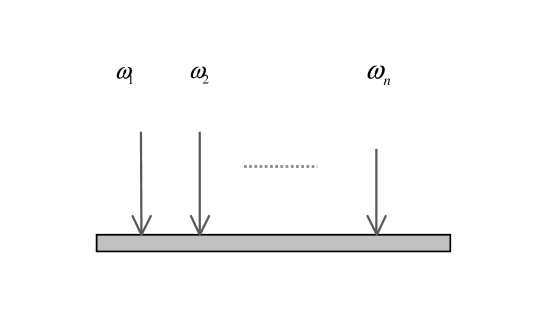
Figure 4: The Walsch-Hadmard duality gate in GMDC.

can be performed by letting the molecule go through a section of the tube with length $L=vt$ while releasing rf radiations with resonance frequencies of all the dubits as shown in Fig.4. After the molecule passes through the QWD, the quantum wave is divided into two sub-waves travelling in different paths where different unitary gate operations are performed. Thus if a molecule passes through path $i$, its internal wave function will change to

$${1\over 2}|\psi\rangle\rightarrow{1\over 2}U_{i}|\psi\rangle,$$ (29)

where the subscript refers to the specific path. Then they recombine to give the wave

$${(U_{1}+U_{2})\over 2}|\psi\rangle.$$ (30)

Then by measuring the internal state of the molecule, for instance using a device such as a Stern-Gerlach apparatus, the computation result is read out. In each path, the computing gate operations can be any operation as that from quantum computation.

VI.2 Nonlinear quantum optics realization schemerabs

We use the polarization of a photon as the two states of a dubit. Photons with different frequency are used to represent different dubits. Thus we need not to consider the identical particle effect of quantum mechanics.

VI.2.1 Basic optical components

First we describe some basic optical components: 1) polarization beamsplitter; 2)the dichromic beamsplitter; 3) parametric down conversion type I; 4) parametric down conversion type II; 5) parametric up-conversion type I; 6) parametric up-conversion type II. The scheme presented here is for the proof-of-principle purpose. In particular, the low efficiency of the up/down conversion is one of the biggest difficulties in the implementation, however we assume them as 100% as no theoretical limit this possibility.

A polarization beamsplitter transmit the vertical polarized light while reflect the horizontal polarized light. When a photon with the following state

$$|\psi\rangle=a|H\rangle+b|V\rangle,$$ (31)

hits a polarization beamsplitter, the state changes to

$$a|H\rangle_{1}+b|V\rangle_{1}\rightarrow a|H\rangle_{3}+b|V\rangle_{2}$$ (32)

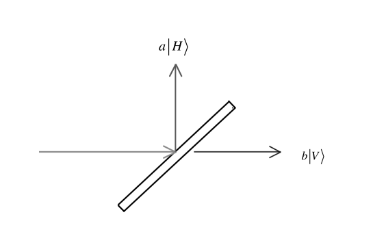
Figure 5: A polarization beamsplitter

as shown in Fig.5.

A dichroic beamsplitter is a device to separate or combine beams of different wavelength. A long wave pass(LWP) dichroic beamsplitter always transmit the longer wavelength wave and reflects the shorter wavelength. A short wave pass(SWP) dichroic beamsplitter always transmits the shorter wavelength and reflects the longer wavelength. When a beam of light with both wavelength $\lambda_{1}$ and $\lambda_{2}$ enters dichroic beamsplitter, one wavelength is reflected and the other is transmitted. Then the two beams are separated so that we can perform individual operations on a specific wavelength photon, for instance a phase modulation, or a polarization modulation. This is very convenient for duality computation. When we inverse the directions of the two beams in a dichroic beamsplitter, we can combine the two separated beams so that they become a single beam with different wavelengths. We can use multiple dichroic beamsplitters to separate out individual wavelength photon. Dichroic beamsplitter is different from QWD in the sense that a dichroic beamsplitter separates two photons with different wavelengths into different paths whereas a QWD divides the wave function for the whole two photons into two parts where in each path the sub-wave describe the two photons.

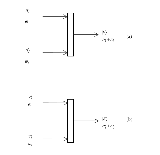
Figure 6: Type I up-conversion. (a) Case 1 of type I SFG; (b) Case 2 of type I SFG.

Sum frequency generation(SFG) is a process in which two photons with frequency $\omega_{1}$ and $\omega_{2}$ respectively are combined to form a single photon with frequency $\omega_{1}+\omega_{2}$ as shown in Fig.6. There are two types according to the polarization states of the photons. In type-I SFG, the process produces a photon with higher energy from two photons with identical polarizations, whereas in type-II SFG, the polarizations of the two input photons are different. Mathematically, for type-I SFG, we have

$$|H\rangle_{1}|H\rangle_{2} \rightarrow|V\rangle_{12},$$

$$|V\rangle_{1}|V\rangle_{2} \rightarrow|H\rangle_{12},$$ (33)

as shown in Fig.6, whereas for two photons with arbitrary polarizations, the change is

$$(a_{1}|H\rangle_{1}+b_{1}|V\rangle_{1})(a_{2}|H\rangle_{2}+b_{2}|V\rangle_{2})\rightarrow a_{1}a_{2}|H\rangle_{12}+b_{1}b_{2}|V\rangle_{12}.$$ (34)

For type-II SFG as shown in Fig.7, the changes are

$$|H\rangle_{1}|V\rangle_{2} \rightarrow|H\rangle_{12},$$

$$|V\rangle_{1}|H\rangle_{2} \rightarrow|V\rangle_{12},$$ (35)

and for two input photons with arbitrary polarization states, the change is

$$(a_{1}|H\rangle_{1}+b_{1}|V\rangle_{1})(a_{2}|H\rangle_{2}+b_{2}|V\rangle_{2})\rightarrow a_{1}b_{1}|H\rangle_{12}+b_{1}a_{2}|V\rangle_{12}.$$ (36)

Here the subscript 12 means the up-converted photon.

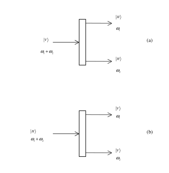
Figure 8: Type I down-conversion: (a) Case 1; (b) Case 2.

Spontaneous parametric down conversion(SPDC) is like the inverse process of SFG and it generates two photons with frequencies $\omega_{1}$ and $\omega_{2}$ on input of a single photon with frequency $\omega_{1}+\omega_{2}$ as shown in Fig.8. There are also two types of SPDC according to the polarizations of the participating photons. In type-I SPDC, the two outgoing photons have the same polarization states whereas in type-II SPDC, the two outgoing photons have different polarization states. Specifically, for type-I SPDC, the changes are

$$|H\rangle_{12}\rightarrow |V\rangle_{1}|V\rangle_{2},$$

$$|V\rangle_{12}\rightarrow |H\rangle_{1}|H\rangle_{2}.$$ (37)

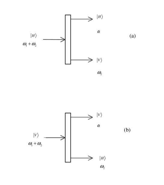
Figure 9: Type II down-conversion: (a) Case 1; (b) Case 2.

For type-II SPDC as shown in Fig.9, the changes are

$$|H\rangle_{12}\rightarrow |H\rangle_{1}|V\rangle_{2},$$

$$|V\rangle_{12}\rightarrow |V\rangle_{1}|H\rangle_{2}.$$ (38)

When the input photon has an arbitrary polarization, the corresponding changes will be the combined effects of both the horizontal polarization and the vertical polarization components. For instance, for type-I SPDC with input photon in state $a|H\rangle_{12}+b|V\rangle_{12}$, the change is

$$a|H\rangle_{12}+b|V\rangle_{12}\rightarrow a|V\rangle_{1}|V\rangle_{2}+b|H\rangle_{1}|H\rangle_{2}.$$ (39)

Similar expressions can be written out explicitly for type-II SPDC.

VI.2.2 Basic Unitary Computing Gates

The single dubit gate operations are the phase rotation gate and the rotation gate. In phase rotation gate, denoted by $P_{\lambda}$ the wave function acquires an arbitrary phase. Operating on a state $a|H\rangle+b|V\rangle$, it changes the state according to

$$P_{\lambda}|\psi\rangle=e^{i\lambda}|\psi\rangle=e^{i\lambda}(a|H\rangle+b|V\rangle).$$ (40)

This can simply be implemented with a variable wave plate.

To rotate the dubit in the 2-dimensional space span by the two orthogonal polarizations, a polarization modulator is sufficient. It rotates the polarization of a photon through angle $\theta$, so a rotation operation $R_{\theta}$ makes the following changes

$$R_{\theta}|H\rangle =\cos\theta|H\rangle+\sin\theta|V\rangle,$$

$$R_{\theta}|V\rangle =-\sin\theta|H\rangle+\cos\theta|V\rangle.$$ (41)

The controlled NOT (CNOT) gate is the most important gate operation in quantum computing and it is also an important gate operation in duality computing. Here we propose a CNOT gate operation scheme using nonlinear quantum optics. It is a generalization of the method for full Bell-basis measurement used in Ref.r20 . It is shown in Fig.10. Two photons with frequencies $\omega_{1}$ and $\omega_{2}$ are two input dubits. They are in a most general superposition of their polarization basis states

$$|\psi_{in}\rangle=a_{00}|H_{1}H_{2}\rangle+a_{01}|H_{1}V_{2}\rangle+a_{10}|V_{1}H_{2}\rangle+a_{11}|V_{1}V_{1}\rangle.$$ (42)

The effect of a CNOT gate is to perform an operation that changes the state to

$$|\psi_{in}\rangle=a_{00}|H_{1}H_{2}\rangle+a_{01}|H_{1}V_{2}\rangle+a_{10}|V_{1}V_{2}\rangle+a_{11}|V_{1}H_{1}\rangle,$$ (43)

that is when the control dubit is in $1$(V), the state of the target dubit is flipped. The nonlinear optics scheme works as follows. First the two photons enters four summed frequency generation(SFG) crystals to generate a single photon with the summed frequency $\omega_{1}+\omega_{2}$. When they enter the type-I SFG group, the crystal with optic axis aligned in the horizontal direction combines the $|H_{1}H_{2}\rangle$ component to form $|V_{12}\rangle$, and the crystal with vertical optic orientation combines the $|V_{1}V_{2}\rangle$ component to form $|H_{12}\rangle$. The component $|H_{1}V_{2}\rangle$ and $|V_{1}H_{2}\rangle$ continue to propagate into the type-II SFG crystal group and they combine to produce $|H_{12}^{\prime}\rangle$ and $|V_{12}^{\prime}\rangle$ respectively. Dichroic beamsplitters, polarization beamsplitters and mirrors are used to separate the different components. Here the state has become

$$a_{00}|V_{12}\rangle+a_{01}|V^{\prime}_{12}\rangle+a_{10}|H^{\prime}_{12}\rangle+a_{11}|H_{12}\rangle,$$ (44)

and thw different components are in different paths. To achieve the CNOT output state, we need to use the SPDC process to generate two photons with frequencies $\omega_{1}$ and $\omega_{2}$ respectively and leaving the $|H_{1}H_{2}\rangle$ and $|H_{1}V_{2}\rangle$ components unchanged, but changes the component $|V_{1}H_{2}\rangle$ and $|V_{1}V_{2}\rangle$. This can be completed by applying the type-I down conversions for $|V_{12}\rangle$ which produces component $|H_{1}H_{2}\rangle$ and for $|H_{12}^{\prime}\rangle$ which produces $|V_{1}V_{2}\rangle$ component respectively. Similarly, the type-II SPDC processes for $|H_{12}\rangle$ and $|V^{\prime}_{12}\rangle$ produces $|H_{1}V_{2}\rangle$ and $|V_{1}H_{2}\rangle$ components respectively. Then the different components are combined and put into two optical paths with frequency $\omega_{1}$ and $\omega_{2}$ respectively. Hence the final state becomes

$$a_{00}|H_{1}H_{2}\rangle+a_{01}|H_{1}V_{2}\rangle+a_{10}|V_{1}V_{2}\rangle+|V_{1}H_{2}\rangle,$$ (45)

the desired state.

The most difficult part is the QWD. We cannot simply let $n$ dubits to pass through a beamsplitter to produce a division of the wave, since there will be $2^{n}$ possibilities as has been pointed out in the preceding section. We need that the $n$ dubits system as a whole be divided into two sub-waves. To achieve this, we need the $n$ dubit photons be generated simultaneously and coherently. First we look at how to produce $n$ dubit photons coherently using SPDC. It can be realized in the setup as shown in Fig.11. Suppose we have a photon with frequency $\omega=\omega_{1}+\omega_{2}+...+\omega_{n}$ and is in state $|V\rangle$. Then we let this photon to pass through a type-I SPDC crystal so that it produces two photons in state $|H_{1}H_{1}^{\prime}\rangle$ where the first photon has frequency $\omega_{1}$ and the second photon has frequency $\omega_{1}^{\prime}=\omega_{2}+...+\omega_{n}$. Then the second photon continues to pass through a type-II SPDC crystal to produce two photons in state $|H_{2}V_{2}^{\prime}\rangle$, with the second photon having frequency $\omega_{2}^{\prime}=\omega_{3}+...+\omega_{n}$. After $n-1$ such SPDC processes, we produce $n$ photons of different frequencies. These $n$ photons can be adjusted so that they arrive in a plane perpendicular to their propagation at the same time. Unitary gate computations can be performed on them using the a series of single dubit operation and the CNOT gate.

Instead of making this $n$ photon wave to divide into two sub-waves with identical internal polarization state, we perform a quantum wave division at the source: we use a beamsplitter before the first SPDC crystal as shown in Fig.12, then the wave function of the photon with $\omega=\omega_{1}+\omega_{2}+...+\omega_{n}$ is divided into sub-waves. A half-wavelength plate is used to compensate the phase difference between transmitted and reflected waves. Each of the sub-wave will further be transformed into a sub-wave of $n$ photons with the coherent photon production process described above. Then the sub-wave in the upper path is

$${1\over\sqrt{2}}|H_{1}H_{2}...H_{n}\rangle_{u},$$ (46)

whereas in the lower path the sub-wave is

$${1\over\sqrt{2}}|H_{1}H_{2}...H_{n}\rangle_{d}.$$ (47)

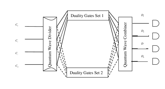
Figure 13: A Global View of Nonlinear Quantum Optics DC.

The whole duality computing process can be shown in Fig.13. The computing unitary gate operations are performed on the upper and lower paths respectively. Then the two path waves are joined finally at the QWC. Because the two paths have the same optical path, the two waves should add up together, therefore the wave after the QWC is

$${1\over 2}\sum_{i=0}^{2^{n}-1}(c_{i,u}+c_{i,d})|i\rangle.$$ (48)

A QWC can be easily constructed by directing the specific photon from the upper path and the lower path so that they coincide in space and time, for instance as in Ref.independent .

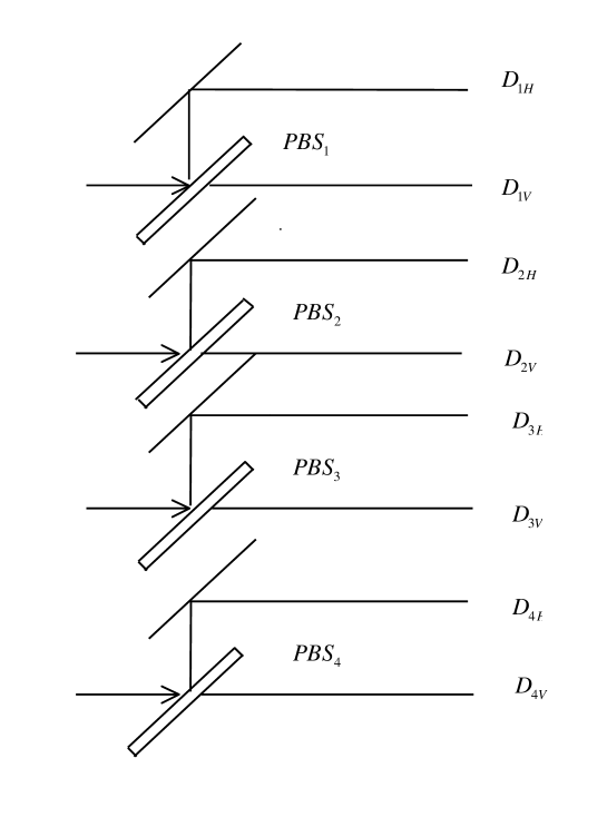
Figure 14: The read-out device in the NODC.

The measurement device is constructed as shown in Fig.14. After the QWD, each dubit is guided to a polarization beamsplitter where the horizontal and vertical components are split and they further travel to two detectors. One of the two detectors will register a click which is a projective measurement for the dubit. We can read out the state of a photon by looking at which detector clicks. If the upper detector clicks, it corresponds to 0, and if the lower detector clicks it corresponds to state 1. Altogether there are $2n$ detectors, and they corresponds to the bit value of the $n$ dubits. This measurement is a projective measurement. In this proof-of-principle design, I assume that all the components are ideal and have 100% efficiency. The up and down conversions are also of 100% efficient.

VII A Single Query Unsorted Database Search and Polynomial Algorithm for NP-complete Problems in Duality Computer

We first present an algorithm that may find an marked item from an unsorted database with a single query. This is an exponentially fast search algorithm. Then we show that NP-complete problem can be reduced to unsorted database search, hence NP-complete problem may become P problem in duality computer. However, the validity of the algorithm depends on the efficiency of measurement for a partial wave function which will be discussed shortly.

VII.1 A duality computer algorithm for unsorted database search

The unsorted database search problem is a benchmark for computing. To find a marked item from an unsorted database of $N$ items, a classical computer requires $O(N)$ steps. A quantum computer requires $O(\sqrt{N})$ steps using the Grover algorithmr25 or an improved algorithm with 100% successful rater26 . By introducing classical parallelism, the problem can be further speeded up modestly. Using the Brüschweiler algorithmbrusch , $O(\ln N)$ steps is required to find the marked state. Using the Xiao-Long algorithm, one needs only a single query to find the marked statexiaolong . However this speedup is achieved at the cost of more computing resources. Namely now there are $O(N)$ quantum computers working in parallel. In general with $N_{2}$ quantum computers working in parallel, the number of queries required to find the marked state is $O(\sqrt{N/N_{2}})$ in a parallelized quantum computingparallel . Though these algorithms achieve speedup by using more resources, they are still useful in ensemble quantum computers such as liquid nuclear magnetic resonance 7qubit .

In duality computer, the speedup may be achieved without the use of additional resource. An algorithm is presented as follows.

1. Prepare the state of the duality computer in the equally distributed state,

$$|\psi_{0}\rangle=\sqrt{1\over N}\sum_{i=0}^{N-1}|i\rangle=\sqrt{1\over N}(|0\rangle+|1\rangle+...+|\tau\rangle+...+|N-1\rangle),$$ (49)

where $\tau$ is the marked item we are searching.

2. Let the duality computer go through QWD, so that it divides the wave into two sub-waves

$$|\psi_{u}\rangle = {1\over 2\sqrt{N}}\sum_{i=0}^{N-1}|i\rangle={1\over 2\sqrt{N}}(|0\rangle+|1\rangle+...+|\tau\rangle+...+|N-1\rangle),$$ (50)

$$|\psi_{d}\rangle = {1\over 2\sqrt{N}}\sum_{i=0}^{N-1}|i\rangle={1\over 2\sqrt{N}}(|0\rangle+|1\rangle+...+|\tau\rangle+...+|N-1\rangle).$$ (51)

3. Apply the query to the lower-path sub-wave, reverse the coefficients of all basis states $|i\rangle$ except the marked state $|\tau\rangle$, the lower sub-wave becomes

$$|\psi_{d}\rangle^{\prime} = {1\over 2\sqrt{N}}(-|0\rangle-|1\rangle+...+|\tau\rangle-...-|N-1\rangle).$$ (52)

No operation is applied to the upper-path sub-wave, it remains in state as in Eq. (50).

4. Combine the sub-waves at the QWC, and the wave becomes

$$|\psi_{f}\rangle=\sqrt{1\over N}|\tau\rangle.$$ (53)

5. Make a read-out measurement, and the marked item $\tau$ will be found with some probability depending on further studies on the measurement of a partial wave function as will be discussed later. In a best case scenario, the measurement gives the marked item with certainty.

The query can be implemented using $O(\ln N)$ number of dubits. As the size of the database $N$ increases, the difficulty in constructing the query increases only logarithmically.

VII.2 Duality algorithm for NP-Complete Problems

According to the Cook-Levin theorem, all NP-complete problems are polynomially equivalent. One can reduce one NP-complete problem in polynomially equivalent steps into another NP-complete problem. Let’s look at the SATISFIABILITY problem, where one needs to find if there are solutions to a logical expression,

$$P(x_{1},x_{2},...x_{n})=1,$$ (54)

of $n$ binary variables. To find its solution, we cast the problem into an unsorted database search problem, though the reverse is not possible in general. The algorithm is as follows

1. Prepare the state of the duality computer in the equally distributed state,

$$|\psi_{0}\rangle=\sqrt{1\over N}\sum_{i=0}^{N-1}|i\rangle=\sqrt{1\over N}(|0\rangle+|1\rangle+...+|\tau_{1}\rangle++|\tau_{2}\rangle...+|N-1\rangle),$$ (55)

where $\tau_{i}$ is one of the item that satisfies the logical equation Eq.(54).

2. Let the duality computer go through QWD, so that it divides the wave into two sub-waves

$$|\psi_{u}\rangle = {1\over 2\sqrt{N}}\sum_{i=0}^{N-1}|i\rangle={1\over 2\sqrt{N}}(|0\rangle+|1\rangle+...+|\tau_{1}\rangle++|\tau_{2}\rangle+...+|N-1\rangle,$$ (56)

$$|\psi_{d}\rangle = {1\over 2\sqrt{N}}\sum_{i=0}^{N-1}|i\rangle={1\over 2\sqrt{N}}(|0\rangle+|1\rangle+...+|\tau_{1}\rangle++|\tau_{2}\rangle+...+|N-1\rangle).$$ (57)

3. Using the logical expression Eq. (54) as a query. This can be implemented by using $O(n)$ number of dubits in polynomial steps. Apply the query to the lower-path sub-wave, reverse the coefficients of all basis states $|i\rangle$ except those that satisfy Eq.(54), the lower sub-wave becomes

$$|\psi_{d}\rangle = {1\over 2\sqrt{N}}(-|0\rangle-|1\rangle-...+|\tau_{1}\rangle+|\tau_{2}\rangle+...-|N-1\rangle).$$ (58)

No operation is applied to the upper-path sub-wave, it remains in state Eq. (56).

4. Combine the sub-waves at the QWC, and the wave becomes

$$|\psi_{f}\rangle=\sum_{i=1}^{m}\sqrt{1\over m}|\tau_{i}\rangle,$$ (59)

where $m$ is the number of items that satisfies the logical expression Eq.(54).

5. Make a read-out measurement, if Eq.(54) is satisfiable one of the marked item $\tau_{i1}$ is found out. If it is not satisfiable, no state is obtained.

6. To find all the solutions to the logical expression, one repeat steps 1, 2, 3, 4. Now we let the wave in Eq. (59) go through a QWD again and divide it into two paths. We inverse the state $|\tau_{i1}\rangle$ in one path and then we combine them in a QWC. Then the $|\tau_{i1}\rangle$ component is deleted from the state Eq.(59). Another measurement reads out a solution other than $\tau_{i1}$. Continuing in this way, all the $m$ solutions to the problem are found.

VII.3 The measurement efficiency for a partial wave function

It is worth mentioning the coefficient in Eq. (53). It can not simply be renormalized to 1. For if the two sub-waves have opposite signs, they will cancel each so that the probability will be zero which corresponds to a dark point in an interference pattern. If the two sub-waves are in phase, then the probability of detection will be the greatest and it will correspond to a bright spot in an interference pattern. Then one would be expected to give the probability of $1/N$ for obtaining the marked state from state in Eq. (53) and this would make the search algorithm useless. However, it is not so simple. It depends on the interpretation of the wave function and the measurement in quantum mechanics. We suggest three possibilities, and the final answer depends on further experiment.

First we point that the probability of finding state $|\tau\rangle$ in a state in Eq. (53) and in state (49) may be different. In Eq. (53), the situation is whether we get a result for a measurement or do not get a result at all, while in Eq. (49), we always get a result which is one of the $N$ basis states, and $\tau$ will have only $1/N$ probability to be the result.

We give three possibilities:

1) The possibility is $1/N$ and there is no difference between Eq. (53) and Eq. (49). This is true for some interpretations of quantum mechanics, for instance in the ignorance interpretation where the particle is actually in some point in space and the probability is because we do not know this knowledge.

2) The probability is 100%, however one has to wait longer time to get a result. This may be reasonable as the measuring process may need some interaction between the duality computer system and the detector. The smaller the wave function exposed to the detector, the longer it takes to get a result.

3) The probability is 100% and it takes about the same period of time to get the result. But it may require that the magnitude of the amplitude be greater than a minimum value. Under the minimum value, the detector will not register a click, hence no particle will be detected when the two-sub-waves are in total cancellation. However when it is bigger than the minimum amount, the detector will register a click as if the whole wave function is exposed to the detector. This can be understood in the giant molecule scheme. If the two sub-waves have opposite signs so that total cancellation takes place, it means that the giant molecule is trapped inside the tube as a standing wave. If partial cancellation occurs, for instance in Eq.(53), the major part of the wave function is inside the tube as standing wave, and only a small part is exposed to the detector. However here we just make measurement on this part of the wave function, the other part of the wave function is not measured and they can not collapse. Hence if no absorption takes place inside the tube, the detector always obtains a result. If detectors were placed everywhere inside the tube, then the detector would have $1/N$ probability to get a result as it is competing with other detectors. However as no competing detectors are present, the detector at the final point will always obtain a result in normal time span. For instance if we have a balloon, and we use a board full of needles to punch it. Any one of the needles can punch the balloon so that collapse it. However we can break the balloon with the same ease if we just use one needle to punch the balloon in just a small area.

As a test, we propose the following thought experiment that may also be performed practically. One traps a single electron in a Penning trap. Then putting different number of detectors inside the Penning trap such as that in Ref.penning , and switch on the detectors study the time period when one of the detectors registers a click. The more the detectors, the larger the electron wave function being measured.

We leave the problem open at this stage, and a detailed discussion will be published elsewhere. For use in computing, the third possibility is preferred, and if it is true duality computer will be the most powerful computing machine so far. It will be interesting to study if it is possible to improve the efficiency by repetition or by placing more detectors at other spatial phase difference points, or using the quantum Zeno effect, in the worst scenario.

However, it should be emphasized that irrespective of the result on the measurement efficiency, the duality computer can be made to work as a quantum computer: the upper and lower sub-waves experience the same gate operation. Thus the computing power of duality computer is at least as powerful as the quantum computer, even in the worst case of the measurement efficiency.

VIII Concluding Remarks

We have proposed a general principle of quantum interference. Whenever the sub-waves of a quantum system, whether single, bound or loose, coincide in space and time, interference may occur.

The quantum computer uses only the particle nature of quantum system, and it does not use the full power of quantum mechanics.

We propose the duality computer. Quantum wave can be divided and recombine. Different computing gate operations can be performed at the different paths. This enables us to perform computation using not only products of unitary operations, but also linear combinations of unitary operations. This provides duality parallelism which may outperform quantum parallelism in quantum computer.

Two conceptual designs of duality computer are proposed. The giant molecule scheme and the nonlinear quantum optics scheme.

Searching a marked item from an unsorted database may require only a single query in duality computer. This is the holy grail of unsorted database search problem.

NP-complete problem can be cast into an unsorted database search problem. Thus NP-complete problem may become P problem in duality computer. This may be the first possible computing machine to answer the question if NP-complete is equivalent to P.

Open problem exists on the detection efficiency in the duality computer. Three possibilities are proposed which are closely related to fundamental issues in quantum mechanics. The final answer depends on further experimental result, though a specific answer is favored for duality computing.

Building a duality computer maybe difficult. However taking into account the enormous power it may provide, experimental endeavors are worthwhile, in particular the test of the general interference principle for complicated quantum systems and to find out the measurement efficiency of a partial wave function.

This work is supported by the National Fundamental Research Program Grant No. 001CB309308, China National Natural Science Foundation Grant No. 10325521, 60433050, and the SRFDP program of Education Ministry of China.

It should be noted that quantum interference also exists in quantum computer, for instance in the Shor algorithm where wanted components are strengthened and unwanted components are suppressed. However, in the quantum computer, unitarity of gate operations are always obeyed. The quantum computer system as a whole exhibits particle nature. The role of quantum interference in quantum computing has been studied by Ekert ekert , Galindo and Martin-Delgado martin , Shiekhshiekh and Finkelsteinshiekh .

Caufield and Shamir proposed an optical computer employing the particle and wave duality nature of light where one or several coherent light sources illuminate an optical system containing the input variables and a detector array that records the outputswpd1 . Our model is different from their model in that the particle wave duality nature is exhibited in a different manner. In the duality computer, the whole quantum system of the computer system exhibits the particle wave duality nature whereas inthe Caufield and Shamir computer model the computer system as a whole does not exhibit the particle wave duality: it is always present there as a particle, and the particle wave duality nature is only exhibited by the individual lights, thus it may be a hybrid computer model of classical computer and quantum computer.

Figure 2: A quantum wave divider and a quantum wave combiner

Figure 10: The CNOT gate in Nonlinear Quantum Optics DC.

Figure 11: Coherent generation of multi-dubits in the Nonlinear Quantum Optics DC using cascade down-conversions

Figure 12: A QWD in Nonlinear Quantum Optics DC. The 4-dubits in the upper path and lower path have identical polarization states.

References

- (1) N. Bohr, The quantum postulate and the recent development of atomic theory, Naturwissenschaften, 16, 245-257 (1928).
- (2) R. F. Feynman, R. B. Leighton, M. Sands, The Feynman Lectures on Physics, Addison-Wesley Publishing Company, Reading, 1963, Vol. 1, p.37-2.
- (3) S. Dürr, T. Nonn and G. Rempe, Origin of quantum-mechanical complementarity probed by a ’which-way’ experiment in an atom interferometer, Nature, (London) 395, 33-37 (1998).
- (4) Thomas Young, Philosophical Transactions of the Royal Society of London, 94, 1-16 (1804)
- (5) C Jönsson,Zeitschrift für Physik 161, 454-474 (1961).
- (6) P G Merli, G F Missiroli and G Pozzi, On the statistical aspect of electron interference phenomena, American Journal of Physics, 44 306-7 (1976)
- (7) A Tonomura, J Endo, T Matsuda, T Kawasaki and H Ezawa, Demonstration of single-electron build-up of an interference pattern, American Journal of Physics, 57, 117-120 (1989).
- (8) D. F. Walls, A simple field theoretic treatment of photon interference, American Journal Physics 45, 952-956 (1977).
- (9) P. A. M. Dirac, The principles of quantum mechanics, 3rd edition, Oxford University Press, Oxford, 1947, P.9
- (10) C. Santori, D. Fattal, J. Vučković, G. S. Solomon and Y. Yamamoto, Indistinguishable photons from a single-photon device, Nature, (London), 419, 594 (2002).
- (11) A. Church, An unsolvable problem of elementary number theory, Am. J. Math. 58, 345 (1936).
- (12) A. M. Turing, On Computable numbers, with an application to the entscheidungsproblem, Proc. Lond. Math. Soc. Ser.2, 442, 230 (1936).
- (13) R. Landauer, IBM J. Res. Develop. 3, 183 (1961); R. W. Keyes and R. Landauer, IBM J. Res. Develop., 14, 152 (1970).
- (14) C. H. Bennett, Logical Reversibility of Computation, IBM J. Res. Develop. 17, 525 (1973).
- (15) P. Benioff, Quantum mechanical models of Turing machines that dissipate no energy, Phys. Rev. Lett. 48, 1581 (1982).
- (16) R. P. Feynman, Simulating physics with computers, Int. J. Thoer. Phys., 21, 467-488, (1982).
- (17) D. Deutsch, Quantum theory, the Church-Turing principle and the universal quantum computer, Proc. R. Soc. Lond. A 400, 97 (1985).
- (18) A. C. C. Yao, Quantum circuit Complexity, in Proc. 34th Annual IEEE Symposium on Foundations of Computer Science, IEEE Press, Picataway, NJ, 1993, pp.352-361.
- (19) S.A. Cook, The complexity of theorem-proving procedures. In Proc. 3rd Annual ACM Symposium on Theory of Computing, pages 151-158, 1971; L. Levin Universalnyie Perebomyie Zadachi, Problemy Peredachi Informatiss, 9 (3): 265-266, 1973.
- (20) W. Wootters and W. Zurek, A simple quantum cannot be cloned, Nature, 299, 802-803 (1982).
- (21) M. Arndt, O. Nairz, J. Vos-Andreae, C. Keller, G. Van der Zouw and A. Zeilinger, Nature, 401, 680-682, (1999)
- (22) Yanhua Shih, Two-photon entanglement and quantum reality, Advances in Atomic, Molecular and Optical, 41, 1-41 (1999).
- (23) P. Zhang and C. P. Sun, Two photon interference and optical free induction decay, arXiv: quant-ph/0209154.
- (24) G. Badurek, H. Rauch and D. Tuppinger, neutron interferometric double-resonance experiment, Phys. Rev. A 34, 2600 (1976).
- (25) C. K. Hong, Z. Y. Ou and L. Mandel, Measurement of subpicosecond time intervals between two photons by interference, Phys. Rev. Lett. , 59, 2044-2046, (1987).
- (26) R. L. Pfleegor and L. Mandel, Phys. Rev. 159, 1084 (1967).
- (27) P. Shor, Algorithms for quantum computation: discrete log and factoring, in Proc. 35th Annual IEEE Symposium on Foundations of Computer Science, IEEE Press, Picataway, NJ, 1994, pp.124-134.
- (28) L. Grover, A fast quantum mechanical algorithm for database search, in Proc. 28th Annual ACM Symposium on Theory of Computing, ACM, New York, 1996, pp.212-219.
- (29) G. L. Long, Grover algorithm with zero failure rate, Phys. Rev. A64, 022307 (2001).
- (30) M. Boyer, G. Brassard, P. Hoyer, and A. Tapp, Strength and weakness of quantum computation, Fortschr. Phys. 46, 493 (1998).
- (31) D. Deutsch, Quantum Computational Networks, Proc. R. Soc. Lond. A425, 73-90 (1989).
- (32) A. Barenco, C. H. Bennett, R. Cleve, D. P. DiVincenzo, N. Margolus, P. Shor, T. Sleator, J. A. Smolin and H. Weinfurter, Phys. Rev. A52, 3457 (1996).
- (33) Y. H. Kim, S. P. Kulik and Y. H. Shih, Quantum teleportation of a polarization state with a complete Bell state measurement, Phys. Rev. Lett. 86, 1370 (2001).
- (34) R. Bruüschweiler, Phys. Rev. Lett. 85, 4815 (2000).
- (35) L. Xiao and G. L. Long, Fetching marked items from an unsorted database using NMR ensemble computing, Phys. Rev. A 66, 052320 (2002).
- (36) Gui Lu Long and L. Xiao, Parallel quantum computing in a single ensemble quantum computer, Phys. Rev. A 69, 052303 (2004)
- (37) G L Long and L Xiao, Experimental realization of a fetching algorithm in a 7-qubit NMR Liouville space computer, J. Chem. Phys. 119, 8473-8481 (2003)
- (38) H. Dehmelt, Less is more: experiments with an individual atomic particle at rest in free space, Ameri. J. Phys. 58, 17-27 (1990)
- (39) This scheme was first reported briefly in an unpublished abstract submitted to SPIE conference ”Fluctuations and Noise in Photonics and Quantum Optics” in 2002 where it was mentioned that in this scheme NP=Prabs .
- (40) A. Ekert, Quantum interferometers as quantum computers Phys. Scripta, T 76: 218-222 (1998)
- (41) A. Galindo, M. A. Martin-Delgado, Information and Computation: Classical and Quantum Aspect, Rev. Mod. Phys. 74: 347-423 (2002).
- (42) A. Shiekh, arXiv:cs.cc/0507003, accepted in Int. J. Theo. Phys.
- (43) H John Caulfield and Joseph Shamir, Wave particle duality considerations inoptical computing, Appl. Optics, 28: 2184 (1989)