Time evolution of the relativistic unstable electromagnetic system in the unified formulation of quantum and kinetic dynamics

Abstract

Description of time evolution of the relativistic unstable electromagnetic system consisting of Fermi - Dirac particle interacting with electromagnetic field, in the framework of the Liouville space extension of quantum mechanics is done. The work was carried out on the basis of Prigogine’s unified formulation of quantum and kinetic dynamics. The eigenvalues problem for the relativistic Hamiltonian of the electromagnetic system was solved. The obtained results can be used as the ground for the further studies of the observed physical processes such as bremsstrahlung, relaxation of excited states of atoms and atomic nuclei, particles decay.

1 Introduction

It is known that the description of physical world on the basis of fundamental classical and quantum theories is defined by the laws of the nature as deterministic, time reversible. The time in the usual formulation of dynamics does not have the chosen direction and the future, and the past are not distinguished. However, it is also noted that the facts given before are in the contradiction to our experience, because the world surrounding us has obvious irreversible nature. In this world the symmetry in the time is disrupted and the future and the past play different roles. Difference between the classical description of the nature and those processes in the nature which we observe creates the conflict situation. I. Prigogine noted that the solution of this problem is impossible (at least accurately) on the basis of the conventional formulation of quantum mechanics. Therefore one should speak about the alternative formulation of dynamics that makes it possible to include the irreversibility in a natural way. In this connection the studies of the irreversible processes at the microscopic level - the microscopic formulation of the irreversibility represents for me the special interest.
The alternative formulation of dynamics found its embodiment in the works of Brussels-Austin group that was headed by I. Prigogine for many years. The authors of the approach deny the conventional opinion that the irreversibility appears only at the macroscopic level, while the microscopic level must be described by the laws, reversed in the time. The mechanism of the asymmetry of processes in the time, which made it possible to accomplish a passage from the reversible dynamics to the irreversible time evolution one was developed. In the approach the law of the increase of entropy is accepted as the fundamental that determines the ”arrow of time”, the difference between the past and the future. Thus, new irreversible dynamics with the disrupted symmetry in the time was formulated. In the approach of Brussels-Austin group the irreversibility is presented as the property of material itself and is not defined by the active role of the observer. From the other side the approach allows to solve the problems, which could not be solved within the framework of classical and quantum mechanics. For example, now we can realize the program of Heisenberg - to solve the eigenvalues problem for the Poincare’s non-integrable systems, which could not be solved within the framework of traditional methods. The approach solves the basic problem, designated by Boltzmann and Planck - to formulate the second law of thermodynamics at the microscopic level.
The general formalism of Brussels-Austin group approach was developed in works [1] - [22]. In these papers the basic ideas of the transition from deterministic dynamics to the irreversible description are formulated. In monographs [1], [2] the universal survey of ideas and principles of the alternative formulation of dynamics is given. A unified formulation of dynamics and thermodynamics is done, for example, in works [4], [5]. It is carried out the study of the non-integrable systems, where the alternative formulation of quantum mechanics for non-integrable systems is proposed [6], [10]. The ”subdynamics” approach is developed in works [3], [7], [8], [11]. In paper [15] the method was adapted for the explicit computation of the eigenvalues problem for the Renyi maps, baker’s transformations, Fridrichs model. The eigenvalues problem for the Liouville operator $L$ is solved in the framework of a complex, irreducible spectral representation [17], [18]. The role of the thermodynamic limit for Large Poincare systems is investigated in work [22]. In works [23], [24], scattering theory in superspace and the three-body scattering theory for finite times is developed. In [25] - [27] in the framework of Friedrichs model the problem of description of quantum unstable states including their dressing is investigated. The problem of the complex spectral representation of Liouville operator in the extended Liouville space outside the Hilbert space is solved. It is shown that the dressed unstable state described by a density matrix can be expressed in the terms of the Gamow vectors. The Gamow vectors are investigated also in works [28] - [32]. The formalism determines the operator of microscopic entropy $M$ and also the time operator $T$ [33]. The time operator $T$ is constructed for a quantum system with unstable particle. In work [34] one-dimensional gas with $\delta$-function interaction is examined. Formalism found its further development in works [40] - [46]. So in work [40] on basis of Friedrichs model a microscopic expression for entropy is obtained. The simple model of interaction harmonic oscillator with a field is developed in work [41]. A problem of quantum decoherence for a particle coupled with a field was considered in work [42]. It was shown that the decoherence in the field is the result of irreversible process. In work [43] analysis of the Hegerfeldt’s theorem is carried out. The analysis of the short-time behaviour of the survival probability in the framework of the Friedrichs model was done in work [44]. The two models of relativistic interaction are examined in the work [45]. The models involve two relativistic quantum fields. They are coupled by the simplest cubic and quadratic interaction. A pair of identical two-level atoms interacting with a scalar field are considered in the work [46]. The questions of irreversibility are developed also in works [47] - [58].
At present in the framework of Prigogine’s ideas the great number of works with the use of different models of interaction was executed. They are the Friedrichs model (see [35] - [39]), the models used interaction of simple cubic, or quadratic form as, for example, in works [28], [45] or $\delta$-function interaction [34]. Therefore, at present moment, it is very interesting and necessary to continue further development of the formalism with the use of realistic relativistic Hamiltonians.
In the paper I examine the possibility of application Brussels-Austin group’s ideas, for the description of time irreversible evolution of the quantum unstable electromagnetic system consisting of Fermi - Dirac particle interacting with electromagnetic field. The model of relaxation of the system with photon emission is investigated. It is important that the Hamiltonian of interaction is determined on the basis of the requirement of the gauge invariance of the model. The definition of the interaction model is done in section 2. In section 3 I present the Liouville formalism, ”subdynamics” approach. In section 4 the initial expression for the density matrix is formulated. The task of the complex spectral representation of Hamiltonian is solved in section 5. The expression for the density matrix describing the evolution of the relativistic, unstable electromagnetic system depending on the time is obtained in section 6. Numerical calculation are given in section 7.

2 Definition of the interaction model

For the operator of fermion field $\psi(x)$ we have the following decomposition [59]

$$\begin{split}&\psi(x)=\psi^{(+)}(x)+\psi^{(-)}(x),\\ \psi^{(+)}(x)&=\frac{1}{(2\pi)^{3/2}}\int\Bigl{(}\frac{m}{p_{0}}\Bigr{)}^{1/2}u^{r}(p)e^{ipx}c_{r}(p)d\textbf{p},\\ \psi^{(-)}(x)&=\frac{1}{(2\pi)^{3/2}}\int\Bigl{(}\frac{m}{p_{0}}\Bigr{)}^{1/2}u^{r}(-p)e^{-ipx}d^{{\dagger}}_{r}(p)d\textbf{p},\end{split}$$ (1)

where $c_{r}(p)$ ($c^{{\dagger}}_{r}(p)$) is the operator of destruction (creation) of the particle, $d^{{\dagger}}_{r}(p)$ ($d_{r}(p)$) is the operator of creation (destruction) of antiparticle. Symbol $"{\dagger}"$ indicates the Hermitian conjugate. Operator $\psi(x)$ satisfies the Dirac equation and evolves according to the Dirac representation, satisfying the expression

$$i\frac{\partial\psi(x)}{\partial t}=[\psi(x),H_{0}].$$ (2)

$H_{0}$ in eq. (2) is a free Hamiltonian. Note that we will write 4 - vectors in the form $A=(\textbf{A},iA_{0})$. In this case the following equalities are valid $A^{2}=\textbf{A}^{2}+A_{4}^{2}=\textbf{A}^{2}-A^{2}_{0}$ and $px=p_{\mu}x_{\mu}=\textbf{px}-p_{0}x_{0}$; $p_{0}=\sqrt{\textbf{p}^{2}+m^{2}}$, $m$ - is mass of the quantum of field. We use units with $\hbar$, and the speed of light $c$ taken to be unity ($\hbar=c=1$). Spinors $u^{r}(p)$, $u^{r}(-p)$ correspond to the particles with helicity $r=\pm 1$.
We determine the operator of electromagnetic field as follows

$$\begin{split}&A_{\mu}(x)=A^{(+)}_{\mu}(x)+A^{(-)}_{\mu}(x),\\ A^{(+)}_{\mu}(x)&=\frac{1}{(2\pi)^{3/2}}\int\frac{1}{\sqrt{2k_{0}}}\sum\limits_{\lambda}e^{\lambda}_{\mu}(k)a_{\lambda}(k)e^{ikx}d\textbf{k},\\ A^{(-)}_{\mu}(x)&=\frac{1}{(2\pi)^{3/2}}\int\frac{1}{\sqrt{2k_{0}}}\sum\limits_{\lambda}e^{\lambda}_{\mu}(k)a^{{\dagger}}_{\lambda}(k)e^{-ikx}d\textbf{k},\end{split}$$ (3)

where $k_{0}=|\textbf{k}|$, $a_{\lambda}(k)$ ($a^{{\dagger}}_{\lambda}(k)$) is the operator of destruction (creation) of $\gamma$-quantum. Operators of the electromagnetic field $A_{\mu}(x)$ evolve according to the Dirac representation as well. Polarization vector $e^{\lambda}_{\mu}(k)$ is determined by the relations

$$e^{\lambda}(k)=(\textbf{e}^{\lambda}(\textbf{k}),0),~{}e^{4}(k)=(\textbf{0},i),~{}\lambda=1,2,3~{}(\text{polarization index}).$$ (4)

$\textbf{e}^{1}(\textbf{k})$, $\textbf{e}^{2}(\textbf{k})$ are unit vectors orthogonal to each other and to the momentum of $\gamma$ - quantum k, $\textbf{e}^{3}(\textbf{k})$ is unit vector directed along vector k.
On the basis of the requirement of gauge invariance of the model the Hamiltonian of interaction must be determined in the conventional form [59] (see also [60])

$$H_{I}(t)=-ie\int N(\overline{\psi}(x)\gamma_{\mu}\psi(x))A_{\mu}(x)d\textbf{x}.$$ (5)

$\gamma_{\mu}$- Hermitian 4$\times$4 matrices ($\gamma_{\mu}$$\gamma_{\nu}$ + $\gamma_{\nu}$$\gamma_{\mu}$ = 2$\delta_{\mu\nu}$, $\gamma^{{\dagger}}_{\mu}=\gamma_{\mu}$), $\overline{\psi}$ = $\psi^{{\dagger}}$$\gamma_{4}$, $N$ is the symbol of the normal ordering of operators, $e$ is the charge of the electron so that the fine structure constant is: $\alpha=e^{2}/4\pi\simeq 1/137$.

3 Liouville formalism, ”subdynamics”

Now let me briefly examine the Liouville formalism (see for example [25], [27]). The time evolution of the density matrix $\rho$ is determined by the Liouville-von Neumann equation

$$i\frac{\partial\rho}{\partial t}=L\rho.$$ (6)

Liouville operator has the form

$$L=H\times 1-1\times H,$$ (7)

here symbol ”$\times$” denotes the operation (A$\times$B)$\rho$=A$\rho$B. In accordance with formula (7), $L$ can be written down in the sum of free part $L_{0}$ that depends on the free Hamiltonian $H_{0}$ and interaction part $L_{I}$ that depends on $H_{I}$: $L=L_{0}+L_{I}$. Let state $|\alpha\rangle$ be the eigenstate of the free Hamiltonian $H_{0}|\alpha\rangle$=$E_{\alpha}|\alpha\rangle$ with the energy $E_{\alpha}$. Then dyad of the states $|\alpha\rangle\langle\beta|$ is the eigenstate of operator $L_{0}$: $L_{0}|\alpha\rangle\langle\beta|=(E_{\alpha}-E_{\beta})|\alpha\rangle\langle\beta|$ or $L_{0}|\nu\rangle\rangle=w^{\nu}|\nu\rangle\rangle$, where the designations $|\nu\rangle\rangle\equiv|\alpha\rangle\langle\beta|$ and $w^{\nu}=E_{\alpha}-E_{\beta}$ were used. $\nu$ is the correlation index: $\nu=0$ if $\alpha=\beta$ - diagonal case (vacuum of correlation) and $\nu\neq 0$ in the remaining off-diagonal case (the details of the theory of correlations can be found in works [2], [10], [25]). In the Liouville space for the dyadic operators we have the relations: inner product defined by (where symbol $Tr$ denotes the calculation of the trace)

$$\langle\langle A|B\rangle\rangle\equiv Tr(A^{{\dagger}}B),$$ (8)

the matrix elements are given by

$$\langle\langle\alpha\beta|A\rangle\rangle\equiv\langle\alpha|A|\beta\rangle,$$ (9)

the biorthogonality and bicompleteness relations have the form

$$\langle\langle\alpha^{{}^{\prime}}\beta^{{}^{\prime}}|\alpha\beta\rangle\rangle=\delta_{\alpha^{\prime}\alpha}\delta_{\beta^{\prime}\beta},~{}\sum\limits_{\alpha,\beta}|\alpha\beta\rangle\rangle\langle\langle\alpha\beta|=1.$$ (10)

It was shown that the description of the irreversible processes at the microscopic level is possible if eigenvalues of Liouvillian $Z^{\nu}_{j}$ are generally complex. Thus, for the Liouville operator $L$ the eigenvalues problem is formulated for the right-eigenstates $|\Psi^{\nu}_{j}\rangle\rangle$ and for the left-eigenstates $\langle\langle\widetilde{\Psi}^{\nu}_{j}|$ [25]

$$L|\Psi^{\nu}_{j}\rangle\rangle=Z^{\nu}_{j}|\Psi^{\nu}_{j}\rangle\rangle,~{}\langle\langle\widetilde{\Psi}^{\nu}_{j}|L=\langle\langle\widetilde{\Psi}^{\nu}_{j}|Z^{\nu}_{j}.$$ (11)

Since $L$ is Hermitian the eigenstates are outside the Hilbert space [27]. In this case the corresponding eigenstates have no Hilbert norm [11], [25]. For $|\Psi^{\nu}_{j}\rangle\rangle$ and $\langle\langle\widetilde{\Psi}^{\nu}_{j}|$ we have the following biorthogonality and bicompleteness relations

$$\langle\langle\widetilde{\Psi}^{\nu}_{j}|\Psi^{\mu}_{j^{\prime}}\rangle\rangle=\delta_{\nu\mu}\delta_{jj^{\prime}},~{}\sum\limits_{\nu,j}|\Psi^{\nu}_{j}\rangle\rangle\langle\langle\widetilde{\Psi}^{\nu}_{j}|=1.$$ (12)

Index $j$ is a degeneracy index since one type of correlation $\nu$ can correspond to different states.
It is shown in work [25] that the eigenstates of $L$ can be written in terms of kinetic operators $C^{\nu}$ and $D^{\nu}$ [61], [62]. Operator $C^{\nu}$ creates correlations other than the $\nu$ correlations, $D^{\nu}$ is destruction operator. The use of the kinetic operators allows to write down the expressions for the eigenstates of Liouville operator in the following form

$$|\Psi^{\nu}_{j}\rangle\rangle=(N^{\nu}_{j})^{1/2}\Phi^{\nu}_{C}|u^{\nu}_{j}\rangle\rangle,~{}\langle\langle\widetilde{\Psi}^{\nu}_{j}|=\langle\langle\widetilde{v}^{\nu}_{j}|\Phi^{\nu}_{D}(N^{\nu}_{j})^{1/2},$$ (13)

where

$$\Phi^{\nu}_{C}\equiv P^{\nu}+C^{\nu},~{}\Phi^{\nu}_{D}\equiv P^{\nu}+D^{\nu}$$ (14)

and $N^{\nu}_{j}$ - is a normalization constant. In the general case the operators $P^{\nu}$ satisfy the following condition [11]

$$P^{\nu}=\sum\limits_{j}|u^{\nu}_{j}\rangle\rangle\langle\langle\widetilde{u}^{\nu}_{j}|,~{}\langle\langle\widetilde{u}^{\nu}_{j}|u^{\mu}_{j^{\prime}}\rangle\rangle=\delta_{\nu\mu}\delta_{jj^{\prime}}.$$ (15)

Similarly for $P^{\nu}$ and $\langle\langle\widetilde{v}^{\nu}_{j}|$ we have

$$P^{\nu}=\sum\limits_{j}|v^{\nu}_{j}\rangle\rangle\langle\langle\widetilde{v}^{\nu}_{j}|,~{}\langle\langle\widetilde{v}^{\nu}_{j}|v^{\mu}_{j^{\prime}}\rangle\rangle=\delta_{\nu\mu}\delta_{jj^{\prime}}.$$ (16)

The determination of the states $|u^{\nu}_{j}\rangle\rangle$, $\langle\langle\widetilde{v}^{\nu}_{j}|$ can be found in work [25]. Substituting (13) in (11) and multiplying $P^{\nu}$ from left on both sides, we obtain [25]

$$\theta^{\nu}_{C}|u^{\nu}_{j}\rangle\rangle=Z^{\nu}_{j}|u^{\nu}_{j}\rangle\rangle,$$ (17)

where

$$\theta^{\nu}_{C}\equiv P^{\nu}L\Phi^{\nu}_{C}=L_{0}P^{\nu}+P^{\nu}L_{I}\Phi^{\nu}_{C}P^{\nu}.$$ (18)

$\theta^{\nu}_{C}$ is the collision operator connected with the kinetic operator $C^{\nu}$. This is non-Hermitian dissipative operator, which plays a main role in nonequilibrium dynamics. As was shown in ref. [11] the case $\nu=0$ leads $\theta^{0}_{C}$ to the collision operator in the Pauli master equation for weakly coupled systems.
Analogously it is possible to obtain equation for operator $\theta^{\nu}_{D}$, which is connected with the destruction kinetic operator $D^{\nu}$.

$$\langle\langle\widetilde{v}^{\nu}_{j}|\theta^{\nu}_{D}=\langle\langle\widetilde{v}^{\nu}_{j}|Z^{\nu}_{j},$$ (19)

where

$$\theta^{\nu}_{D}\equiv L_{0}P^{\nu}+P^{\nu}\Phi^{\nu}_{D}L_{I}P^{\nu}.$$ (20)

Comparing eqs. (11), (17), (19) we can see that $|u^{\nu}_{j}\rangle\rangle$ and $\langle\langle\widetilde{v}^{\nu}_{j}|$ are eigenstates of collision operator $\theta^{\nu}_{C(D)}$ with the same eigenvalues $Z^{\nu}_{j}$ as $L$.
Thus, determination of the eigenvalues problem for the Liouville operator $L$ outside the Hilbert space leads to the connection of quantum mechanics with kinetic dynamics.
Operators $\Phi^{\nu}_{C}$, $\Phi^{\nu}_{D}$ satisfy so-called ”nonlinear Lippmann-Schwinger equation”. For the $\Phi^{\nu}_{C}$ we have [25]

$$\Phi^{\nu}_{C}=P^{\nu}+\sum\limits_{\mu\neq\nu}P^{\mu}\frac{-1}{w^{\mu}-w^{\nu}-i\varepsilon_{\mu\nu}}[L_{I}\Phi^{\nu}_{C}-\Phi^{\nu}_{C}L_{I}\Phi^{\nu}_{C}]P^{\nu},$$ (21)

where the time ordering is introduced. For the determination of the sign of the infinitesimals $\varepsilon_{\mu\nu}$ it is necessary to determine the degree of correlation $d_{\mu(\nu)}$. This was defined as the minimum number of interactions $L_{I}$ by which a given state can reach the vacuum of correlation. It is assumed that the directions to the higher degrees of correlation are oriented in the future, and the directions to the lowest degrees of correlation are oriented in the past. This leads to the relations [25], [63]

$$\varepsilon_{\mu\nu}=+\varepsilon~{}\text{if}~{}d_{\mu}\geq d_{\nu}~{}(t>0);~{}\varepsilon_{\mu\nu}=-\varepsilon~{}\text{if}~{}d_{\mu}<d_{\nu}~{}(t<0).$$ (22)

For the $\Phi^{\nu}_{D}$ we have the equation

$$\Phi^{\nu}_{D}=P^{\nu}+P^{\nu}[\Phi^{\nu}_{D}L_{I}-\Phi^{\nu}_{D}L_{I}\Phi^{\nu}_{D}]\sum\limits_{\mu\neq\nu}P^{\mu}\frac{1}{w^{\nu}-w^{\mu}-i\varepsilon_{\nu\mu}}.$$ (23)

Eqs. (21), (23) determine the kinetic operators of creation $C^{\nu}$ and destruction $D^{\nu}$ as follows

$$\begin{split}C^{\nu}&=\sum\limits_{\mu\neq\nu}P^{\mu}\frac{-1}{w^{\mu}-w^{\nu}-i\varepsilon_{\mu\nu}}[L_{I}\Phi^{\nu}_{C}-\Phi^{\nu}_{C}L_{I}\Phi^{\nu}_{C}]P^{\nu},\\ D^{\nu}&=P^{\nu}[\Phi^{\nu}_{D}L_{I}-\Phi^{\nu}_{D}L_{I}\Phi^{\nu}_{D}]\sum\limits_{\mu\neq\nu}P^{\mu}\frac{1}{w^{\nu}-w^{\mu}-i\varepsilon_{\nu\mu}}.\end{split}$$ (24)

The spectral representation of the Liouville operator can be written down in the form

$$L=\sum\limits_{\nu,j}Z^{\nu}_{j}|\Psi^{\nu}_{j}\rangle\rangle\langle\langle\widetilde{\Psi}^{\nu}_{j}|.$$ (25)

In the Brussels-Austin group approach ”subdynamics” is called the construction of a complete set of spectral projectors $\Pi^{\nu}$  [8], [47], [51]

$$\Pi^{\nu}=\sum\limits_{j}|\Psi^{\nu}_{j}\rangle\rangle\langle\langle\widetilde{\Psi}^{\nu}_{j}|.$$ (26)

The projectors $\Pi^{\nu}$ satisfy the following relations

$$\begin{split}&\Pi^{\nu}L=L\Pi^{\nu},~{}(\text{commutativity});~{}\sum\limits_{\nu}\Pi^{\nu}=1,~{}(\text{completeness});\\ &\Pi^{\nu}\Pi^{\nu^{\prime}}=\Pi^{\nu}\delta_{\nu\nu^{\prime}},~{}(\text{orthogonality});~{}\Pi^{\nu}=(\Pi^{\nu})^{\ast},~{}(\text{star-Hermiticity}),\end{split}$$ (27)

where the action ”$\ast$” corresponds to the ”star” conjugation, which is Hermitian conjugation plus the change $\varepsilon_{\mu\nu}\rightarrow\varepsilon_{\nu\mu}$ [10] [11]. Oprerator $\Pi^{\nu}$ can be represented in the following form [25]

$$\Pi^{\nu}=(P^{\nu}+C^{\nu})A^{\nu}(P^{\nu}+D^{\nu}),$$ (28)

where $A^{\nu}$ is the star-Hermitian operator

$$A^{\nu}=P^{\nu}(P^{\nu}+D^{\nu}C^{\nu})^{-1}P^{\nu}.$$ (29)

Taking (27) it is possible to write down the density matrix $\rho$ as follows

$$\rho=\sum\limits_{\nu}\Pi^{\nu}\rho=\sum\limits_{\nu}\rho^{\nu},$$ (30)

where $\rho^{\nu}=\Pi^{\nu}\rho$. Projectors $\Pi^{\nu}$ can be associated with the introduction of the concept of ”subdynamics” because the components $\rho^{\nu}$ satisfy separate equations. In the framework of the ”subdynamics” approach the time evolution of the density matrix has the form (see, for example, work [11])

$$\begin{split}&\rho^{\nu}(t)\equiv\Pi^{\nu}\rho(t)=exp(-iLt)\Pi^{\nu}\rho(0)=\\ &=(P^{\nu}+C^{\nu})e^{-i\theta^{\nu}_{C}t}A^{\nu}(P^{\nu}+D^{\nu})\rho(0).\end{split}$$ (31)

4 Time evolution of the density matrix

Multiplying $\Pi^{\nu}$ and $P^{\nu}$ from the left on both sides of eq. (6) we obtain

$$i\frac{\partial}{\partial t}P^{\nu}\rho^{\nu}=P^{\nu}L\rho^{\nu}.$$ (32)

Let operators $Q^{\nu}$ determine subspace ortogonal $P^{\nu}$. The states belonging to subspace $Q^{\nu}$ have a degree of correlation differing from those which have the states belonging to subspace $P^{\nu}$

$$P^{\nu}Q^{\nu}=Q^{\nu}P^{\nu}=0,$$ (33)

$$~{}P^{\nu}+Q^{\nu}=1.$$ (34)

Using oprerators $P^{\nu}$ and $Q^{\nu}$ we can rewrite eqs. (24): $C^{\nu}=Q^{\nu}C^{\nu}P^{\nu}$, $D^{\nu}=P^{\nu}D^{\nu}Q^{\nu}$. It is easy to see that operators $C^{\nu}$ describe transitions from $P^{\nu}$ correlation subspace to the $Q^{\nu}$ correlation subspace and operators $D^{\nu}$ describe transitions from the correlation subspaces other than $\nu$ to the $\nu$ subspace. The expressions (28), (32) and (34) result into [25]

$$i\frac{\partial}{\partial t}P^{\nu}\rho^{\nu}=\theta^{\nu}_{C}P^{\nu}\rho^{\nu}.$$ (35)

The case $\nu$=0 leads (35) to the kinetic Pauli master equation for $P^{\nu}\rho^{\nu}$ - component. Eq. (35) describes the time irreversible evolution of the unstable state. Our great interest is to investigate eq. (35) for the system of interacting relativistic Fermi - Dirac particle and electromagnetic field. For this purpose we will obtain the Liouville - von Neumann equation for $P^{\nu}\rho^{\nu}$- component in the Dirac representation. In the Dirac representation for eq. (35) we have

$$i\frac{\partial}{\partial t}P^{\nu}\rho^{\nu}(t)=P^{\nu}L_{I}(t)C^{\nu}P^{\nu}[P^{\nu}\rho^{\nu}(t)].$$ (36)

Determining operator

$$\vartheta^{\nu}(t)\equiv P^{\nu}L_{I}(t)C^{\nu}P^{\nu}$$ (37)

for eq. (36) we get

$$i\frac{\partial}{\partial t}P^{\nu}\rho^{\nu}(t)=\vartheta^{\nu}(t)P^{\nu}\rho^{\nu}(t),$$ (38)

where the previous designations of operators are preserved.
The general solution of eq. (38) can be found after examining the equivalent integral equation. The solution of eq. (38) we will search for the component $P^{\nu}\rho^{\nu}(t)$

$$P^{\nu}\rho^{\nu}(t)=P^{\nu}\rho^{\nu}(t_{0})~{}+~{}(-i)\int\limits^{t}_{t_{0}}dt_{1}\vartheta^{\nu}(t_{1})P^{\nu}\rho^{\nu}(t_{1}),$$ (39)

where $P^{\nu}\rho^{\nu}(t_{0})$ is the component into initial $t=t_{0}$ moment of the time. Substituting in the right side of the expression (39) instead of $P^{\nu}\rho^{\nu}(t_{1})$ the sum

$$P^{\nu}\rho^{\nu}(t_{0})~{}+~{}(-i)\int\limits^{t_{1}}_{t_{0}}dt_{2}\vartheta^{\nu}(t_{2})P^{\nu}\rho^{\nu}(t_{2})$$ (40)

and consecutively continuing this procedure we find

$$\begin{split}&P^{\nu}\rho^{\nu}(t)=\Bigl{(}1~{}+~{}(-i)\int\limits^{t}_{t_{0}}dt_{1}\vartheta^{\nu}(t_{1})~{}+~{}(-i)^{2}\int\limits^{t}_{t_{0}}\int\limits^{t_{1}}_{t_{0}}dt_{1}dt_{2}\vartheta^{\nu}(t_{1})\vartheta^{\nu}(t_{2})~{}+~{}\\ &...~{}+~{}(-i)^{n}\int\limits^{t}_{t_{0}}\int\limits^{t_{1}}_{t_{0}}~{}...~{}\int\limits^{t_{n-1}}_{t_{0}}dt_{1}dt_{2}~{}...~{}dt_{n}\vartheta^{\nu}(t_{1})\vartheta^{\nu}(t_{2})~{}...~{}\vartheta^{\nu}(t_{n})~{}+~{}...\Bigr{)}\times\\ &\times P^{\nu}\rho^{\nu}(t_{0}).\end{split}$$ (41)

The obtained expression can be written down in the form

$$P^{\nu}\rho^{\nu}(t)=\Omega^{\nu}(t,~{}t_{0})P^{\nu}\rho^{\nu}(t_{0}),$$ (42)

where

$$\Omega^{\nu}(t,~{}t_{0})=\sum\limits^{\infty}_{n=0}(-i)^{n}\int\limits^{t}_{t_{0}}\int\limits^{t_{1}}_{t_{0}}~{}...~{}\int\limits^{t_{n-1}}_{t_{0}}dt_{1}dt_{2}~{}...~{}dt_{n}\vartheta^{\nu}(t_{1})\vartheta^{\nu}(t_{2})~{}...~{}\vartheta^{\nu}(t_{n}).$$ (43)

Operator $\Omega^{\nu}(t,~{}t_{0})$ in expression (42) plays the role of the evolution operator. The non-Hermitian operator $\Omega^{\nu}(t,~{}t_{0})$ determines the time irreversible evolution of the density matrix - the time irreversible evolution of the relativistic unstable state.

5 Complex spectral representation of Hamiltonian

Let me examine the eigenvalues problem for the Hamiltonian $H=H_{0}+H_{I}$. As for the Liouville operator the problem will be formulated outside the Hilbert space. In this case as earlier we must distinguish equations for the right-eigenstates $|\varphi_{\gamma}\rangle$ and for the left-eigenstates $\langle\widetilde{\varphi}_{\gamma}|$ of Hamiltonian, where $\gamma$ is the index of the state

$$(H_{0}+H_{I})|\varphi_{\gamma}\rangle=Z_{\gamma}|\varphi_{\gamma}\rangle,~{}\langle\widetilde{\varphi}_{\gamma}|(H_{0}+H_{I})=\langle\widetilde{\varphi}_{\gamma}|Z_{\gamma},$$ (44)

eigenvalue $Z_{\gamma}$ is the complex number. Since $H$ is Hermitian the corresponding eigenstates $|\varphi_{\gamma}\rangle$, $\langle\widetilde{\varphi}_{\gamma}|$ have no Hilbert norm.

$$<\varphi_{\gamma}\mid\varphi_{\gamma}>=<{{\tilde{\varphi}}_{\gamma}}\mid{\tilde{\varphi}_{\gamma}}>=0.$$ (45)

The ”usual” norms of the states $|\varphi_{\gamma}\rangle$, $\langle\widetilde{\varphi}_{\gamma}|$ disappear as required to preserve the Hermiticity of $H$ [10] (the details of the complex eigenvalues problem can be found in works [2], [26]). Let me write down the Hamiltonian of interaction in the form $H_{I}=gV$, determining explicitly coupling constant $g$. The value of coupling constant depends on the model of interaction and will be determined later. Solutions of the eqs. (44) can be found after presenting values $|\varphi_{\gamma}\rangle$, $\langle\widetilde{\varphi}_{\gamma}|$, $Z_{\gamma}$ in the perturbation series

$$|\varphi_{\gamma}\rangle=\sum\limits_{n=0}^{\infty}g^{n}|\varphi_{\gamma}^{(n)}\rangle,~{}\langle\widetilde{\varphi}_{\gamma}|=\sum\limits_{n=0}^{\infty}g^{n}\langle\widetilde{\varphi}_{\gamma}^{(n)}|,~{}Z_{\gamma}=\sum\limits_{n=0}^{\infty}g^{n}Z_{\gamma}^{(n)},$$ (46)

where

$$|\varphi_{\gamma}^{(0)}\rangle=|\gamma\rangle,~{}\langle\widetilde{\varphi}_{\gamma}^{(0)}|=\langle\gamma|,~{}Z_{\gamma}^{(0)}=E_{\gamma}.$$ (47)

As it was shown in ref. [10] from relations (46), (47) we can obtain

$$Z_{\gamma}^{(n)}=\langle\gamma|V|\varphi_{\gamma}^{(n-1)}\rangle~{}-~{}\sum\limits_{l=1}^{n-1}Z_{\gamma}^{(l)}\langle\gamma|\varphi_{\gamma}^{(n-1)}\rangle,$$ (48)

$$\langle\beta|\varphi_{\gamma}^{(n)}\rangle=\frac{-1}{E_{\beta}-E_{\gamma}-i\varepsilon_{\beta\gamma}}(\langle\beta|V|\varphi_{\gamma}^{(n-1)}\rangle~{}-~{}\sum\limits_{l=1}^{n}Z_{\gamma}^{(l)}\langle\beta|\varphi_{\gamma}^{(n-1)}\rangle),$$ (49)

where in accordance with Brussels - Austin group approach the time ordering is introduced. The sign of infinitesimal $\varepsilon_{\beta\gamma}$ depends on the direction of the processes: the transition $\gamma\rightarrow\beta$ we will associate with $\varepsilon_{\beta\gamma}=\varepsilon>0$.
Define $|\gamma\rangle$ as a bare state, which corresponds to relativistic Fermi-Dirac particle and $|\beta\rangle$ as a state consisting of the bare Fermi-Dirac particle and photon: $|\gamma\rangle\equiv|\mathbf{p},r\rangle$, $|\beta\rangle\equiv|\mathbf{p}^{\prime},r^{\prime};\mathbf{k},\lambda\rangle$, where $|\mathbf{p},r\rangle$ refers to a one - particle state, $|\mathbf{p}^{\prime},r^{\prime};\mathbf{k},\lambda\rangle$ is a two - particles state, $\mathbf{p}$ $(\mathbf{p}^{\prime})$, $r$ ($r^{\prime}$) - momentum and helicity of the particle and $\mathbf{k}$, $\lambda$ - momentum and polarization index of photon. In the model, states $|\mathbf{p},r\rangle$ $(|\mathbf{p}^{\prime},r^{\prime}\rangle)$, $|\mathbf{k},\lambda\rangle$ are eigenstates of the free Hamiltonian $H_{0}$: $H_{0}|\mathbf{p},r\rangle=E_{\mathbf{p}}|\mathbf{p},r\rangle$, $H_{0}|\mathbf{k},\lambda\rangle=\omega_{\mathbf{k}}|\mathbf{k},\lambda\rangle$ with $E_{\mathbf{p}}=\sqrt{\mathbf{p}^{2}+m^{2}}$ and $\omega_{\mathbf{k}}=|\mathbf{k}|$ ($m$ - Fermi-Dirac particle’s mass). Hamiltonian $H_{I}$ is determined by the expression (5), $g\equiv e$ is the charge of the electron. Substituting the expressions for $\psi(x)$ (1), $A_{\mu}(x)$ (3) in (48), multiplying by $e^{n}$ and summing with respect to $n$, we obtain

$$\begin{split}&Z_{\mathbf{p},r}=E_{\mathbf{p}}~{}-~{}ie\frac{m}{(2\pi)^{3/2}}\int\sum\limits_{\lambda^{\prime},r^{\prime}}\frac{d\mathbf{p}^{\prime}d\mathbf{k}^{\prime}}{(E_{\mathbf{p}}E_{\mathbf{p}^{\prime}}2\omega_{\mathbf{k}^{\prime}})^{1/2}}~{}\delta(\mathbf{p}^{\prime}-\mathbf{p}+\mathbf{k}^{\prime})~{}\times~{}\\ &\times e^{i(E_{\mathbf{p}}-E_{\mathbf{p}^{\prime}}-\omega_{\mathbf{k}^{\prime}})t}e^{\lambda^{\prime}}_{\mu}(k^{\prime})\overline{u}^{r}(p)\gamma_{\mu}u^{r^{\prime}}(p^{\prime})\frac{\langle\mathbf{p}^{\prime},r^{\prime};~{}\mathbf{k}^{\prime},\lambda^{\prime}|\varphi_{\mathbf{p},r}\rangle}{\langle\mathbf{p},r|\varphi_{\mathbf{p},r}\rangle}.\end{split}$$ (50)

The expression for $\langle\mathbf{p}^{\prime},r^{\prime};~{}\mathbf{k}^{\prime},\lambda^{\prime}|\varphi_{\mathbf{p},r}\rangle$ can be obtained from relation (49). In our case we get

$$\begin{split}&\langle\mathbf{p}^{\prime},r^{\prime};~{}\mathbf{k}^{\prime},\lambda^{\prime}|\varphi_{\mathbf{p},r}\rangle=ie\frac{m}{(2\pi)^{3/2}}\int\sum\limits_{r^{\prime\prime}}\frac{d\mathbf{p}^{\prime\prime}}{(E_{\mathbf{p}^{\prime}}E_{\mathbf{p}^{\prime\prime}}2\omega_{\mathbf{k}^{\prime}})^{1/2}}~{}\times\\ &\times\delta(\mathbf{p}^{\prime\prime}-\mathbf{p}^{\prime}-\mathbf{k}^{\prime})e^{i(E_{\mathbf{p}^{\prime}}-E_{\mathbf{p}^{\prime\prime}}+\omega_{\mathbf{k}^{\prime}})t}e^{\lambda^{\prime}}_{\mu}(k^{\prime})\overline{u}^{r^{\prime}}(p^{\prime})\gamma_{\mu}u^{r^{\prime\prime}}(p^{\prime\prime})~{}\times\\ &\times\frac{\langle\mathbf{p}^{\prime\prime},r^{\prime\prime}|\varphi_{\mathbf{p},r}\rangle}{E_{\mathbf{p}^{\prime},\mathbf{k}^{\prime}}-Z_{\mathbf{p},r}-i\varepsilon},\end{split}$$ (51)

where $E_{\mathbf{p}^{\prime},\mathbf{k}^{\prime}}\equiv E_{\mathbf{p}^{\prime}}+\omega_{\mathbf{k}^{\prime}}$. Substituting the expression (51) into (50) for $Z_{\mathbf{p},r}$ we obtain

$$\begin{split}&Z_{\mathbf{p},r}=E_{\mathbf{p}}~{}+~{}e^{2}\frac{m^{2}}{(2\pi)^{3}}\int\sum\limits_{\lambda^{\prime},r^{\prime}}\frac{d\mathbf{p}^{\prime}d\mathbf{k}^{\prime}}{E_{\mathbf{p}}E_{\mathbf{p}^{\prime}}2\omega_{\mathbf{k}^{\prime}}}~{}\delta(\mathbf{p}^{\prime}-\mathbf{p}+\mathbf{k}^{\prime})~{}\times~{}\\ &\times~{}\frac{e^{\lambda^{\prime}}_{\mu}(k^{\prime})\overline{u}^{r}(p)\gamma_{\mu}u^{r^{\prime}}(p^{\prime})e^{\lambda^{\prime}}_{\nu}(k^{\prime})\overline{u}^{r^{\prime}}(p^{\prime})\gamma_{\nu}u^{r}(p)}{E_{\mathbf{p}^{\prime},\mathbf{k}^{\prime}}-Z_{\mathbf{p},r}-i\varepsilon}~{}.\end{split}$$ (52)

Using the formal expression $\frac{1}{w\pm i\varepsilon}\rightarrow\wp\frac{1}{w}\mp i\pi\delta(w)$ rewrite (52) in the form

$$Z_{\mathbf{p},r}=\widetilde{E}_{\mathbf{p},r}~{}-~{}i\gamma_{\mathbf{p},r},$$ (53)

where

$$\begin{split}&\widetilde{E}_{\mathbf{p},r}=E_{\mathbf{p}}~{}+~{}e^{2}\frac{m^{2}}{(2\pi)^{3}}\wp\int\sum\limits_{\lambda^{\prime},r^{\prime}}\frac{d\mathbf{p}^{\prime}d\mathbf{k}^{\prime}}{E_{\mathbf{p}}E_{\mathbf{p}^{\prime}}2\omega_{\mathbf{k}^{\prime}}}~{}\delta(\mathbf{p}^{\prime}-\mathbf{p}+\mathbf{k}^{\prime})~{}\times~{}\\ &\times~{}\frac{e^{\lambda^{\prime}}_{\mu}(k^{\prime})\overline{u}^{r}(p)\gamma_{\mu}u^{r^{\prime}}(p^{\prime})e^{\lambda^{\prime}}_{\nu}(k^{\prime})\overline{u}^{r^{\prime}}(p^{\prime})\gamma_{\nu}u^{r}(p)}{E_{\mathbf{p}^{\prime},\mathbf{k}^{\prime}}-Z_{\mathbf{p}r}}\end{split}$$ (54)

is the renormalized energy ($\wp$ stands for the principal part) and

$$\begin{split}&\gamma_{\mathbf{p},r}~{}=~{}-e^{2}\frac{m^{2}}{8\pi^{2}}\int\sum\limits_{\lambda^{\prime},r^{\prime}}\frac{d\mathbf{p}^{\prime}d\mathbf{k}^{\prime}}{E_{\mathbf{p}}E_{\mathbf{p}^{\prime}}2\omega_{\mathbf{k}^{\prime}}}~{}\delta(\mathbf{p}^{\prime}-\mathbf{p}+\mathbf{k}^{\prime})~{}\times~{}\\ &\times~{}e^{\lambda^{\prime}}_{\mu}(k^{\prime})\overline{u}^{r}(p)\gamma_{\mu}u^{r^{\prime}}(p^{\prime})e^{\lambda^{\prime}}_{\nu}(k^{\prime})\overline{u}^{r^{\prime}}(p^{\prime})\gamma_{\nu}u^{r}(p)\delta(E_{\mathbf{p}^{\prime},\mathbf{k}^{\prime}}-Z_{\mathbf{p},r}).\end{split}$$ (55)

The expression (52) leads to the relation

$$\begin{split}&E_{\mathbf{p}}-Z_{\mathbf{p},r}~{}-~{}e^{2}\frac{m^{2}}{(2\pi)^{3}}\int\sum\limits_{\lambda^{\prime},r^{\prime}}\frac{d\mathbf{p}^{\prime}d\mathbf{k}^{\prime}}{E_{\mathbf{p}}E_{\mathbf{p}^{\prime}}2\omega_{\mathbf{k}^{\prime}}}~{}\delta(\mathbf{p}^{\prime}-\mathbf{p}+\mathbf{k}^{\prime})~{}\times~{}\\ &\times~{}\frac{|e^{\lambda^{\prime}}_{\mu}(k^{\prime})\overline{u}^{r}(p)\gamma_{\mu}u^{r^{\prime}}(p^{\prime})|^{2}}{E_{\mathbf{p}^{\prime},\mathbf{k}^{\prime}}-Z_{\mathbf{p},r}-i\varepsilon}=0.\end{split}$$ (56)

From eq. (56) we can obtain the connection

$$\frac{1}{E_{\mathbf{p}^{\prime},\mathbf{k}^{\prime}}-Z_{\mathbf{p},r}-i\varepsilon}=\frac{1}{E_{\mathbf{p}^{\prime},\mathbf{k}^{\prime}}-E_{\mathbf{p}}-i\varepsilon}+O(e),$$ (57)

where $O(e)$ determines the terms of higher orders on $e$. Limiting the expression (55) by order $e^{2}$ we have

$$\begin{split}&\gamma_{\mathbf{p},r}\approx~{}e^{2}\frac{m^{2}}{8\pi^{2}}\int\sum\limits_{\lambda^{\prime},r^{\prime}}\frac{d\mathbf{p}^{\prime}d\mathbf{k}^{\prime}}{E_{\mathbf{p}}E_{\mathbf{p}^{\prime}}2\omega_{\mathbf{k}^{\prime}}}~{}\delta(\mathbf{p}^{\prime}-\mathbf{p}+\mathbf{k}^{\prime})\delta(E_{\mathbf{p}^{\prime},\mathbf{k}^{\prime}}-E_{\mathbf{p}})~{}\times~{}\\ &\times~{}|e^{\lambda^{\prime}}_{\mu}(k^{\prime})\overline{u}^{r}(p)\gamma_{\mu}u^{r^{\prime}}(p^{\prime})|^{2}~{}>~{}0,\end{split}$$ (58)

where for the photon $\lambda^{\prime}=1,2.$ Since the expressions (56) (57) contain two complex terms $i\gamma_{\mathbf{p},r}$ and $i\varepsilon$, which determine a pole in the lower half plane and a pole in the upper half plane, the operation of integration of the expressions, which contain the values of the form $\frac{1}{E_{\mathbf{p}^{\prime},\mathbf{k}^{\prime}}-Z_{\mathbf{p},r}-i\varepsilon}$ is accepted to determine as follows [10], [11], [48]: we first have to evaluate the integration on the upper half-plane $(C^{+})$ and then the limit of $z\rightarrow-i\gamma_{\mathbf{p},r}$ must be taken. For example the integration over $E_{\mathbf{p}^{\prime}}$ with a test function $g(E_{\mathbf{p}^{\prime}})$ can be presented as follows

$$\begin{split}&\lim\limits_{z\rightarrow-i\gamma_{\mathbf{p},r}}\Bigr{(}\int\limits_{0}^{\infty}dE_{\mathbf{p}^{\prime}}\frac{g(E_{\mathbf{p}^{\prime}})}{E_{\mathbf{p}^{\prime}}+\omega_{\mathbf{k}^{\prime}}-\widetilde{E}_{\mathbf{p}}~{}-~{}z}\Bigl{)}_{z\in C^{+}}\equiv\\ &\equiv\int\limits_{0}^{\infty}dE_{\mathbf{p}^{\prime}}\frac{g(E_{\mathbf{p}^{\prime}})}{(E_{\mathbf{p}^{\prime}}+\omega_{\mathbf{k}^{\prime}}-\widetilde{E}_{\mathbf{p}}~{}-~{}z)^{+}_{-i\gamma_{\mathbf{p},r}}}.\end{split}$$ (59)

This special feature will be used below for the determination of the expression for the density matrix.

6 Expression for the density matrix

Determination of the expression (42) we will carry out for the diagonal ($\nu$=0) matrix element of the form $\langle\langle\gamma\gamma|\rho^{0}(t)\rangle\rangle\equiv\rho^{0}_{\gamma\gamma}(t)$. Let initial moment of time be zero. In this case the expression (42) can be represented as follows

$$\begin{split}&\rho^{0}_{\gamma\gamma}(t)=\rho^{0}_{\gamma\gamma}(0)~{}+~{}(-i)\int\limits^{t}_{0}dt_{1}\langle\langle\gamma\gamma|\vartheta^{0}(t_{1})|\alpha\alpha\rangle\rangle\rho^{0}_{\alpha\alpha}(0)~{}+~{}\\ &+~{}(-i)^{2}\int\limits^{t}_{0}\int\limits^{t_{1}}_{0}dt_{1}dt_{2}\langle\langle\gamma\gamma|\vartheta^{0}(t_{1})|\gamma^{\prime}\gamma^{\prime}\rangle\rangle\langle\langle\gamma^{\prime}\gamma^{\prime}|\vartheta^{0}(t_{2})|\alpha\alpha\rangle\rangle\rho^{0}_{\alpha\alpha}(0)~{}+~{}\\ &+~{}(-i)^{3}\int\limits^{t}_{0}\int\limits^{t_{1}}_{0}\int\limits^{t_{2}}_{0}dt_{1}dt_{2}dt_{3}\langle\langle\gamma\gamma|\vartheta^{0}(t_{1})|\gamma^{\prime}\gamma^{\prime}\rangle\rangle\langle\langle\gamma^{\prime}\gamma^{\prime}|\vartheta^{0}(t_{2})|\gamma^{\prime\prime}\gamma^{\prime\prime}\rangle\rangle\times~{}\\ &\times\langle\langle\gamma^{\prime\prime}\gamma^{\prime\prime}|\vartheta^{0}(t_{3})|\alpha\alpha\rangle\rangle\rho^{0}_{\alpha\alpha}(0)~{}+~{}...,~{}\end{split}$$ (60)

where summation (integration) over all internal indices $\gamma^{\prime}$, $\gamma^{\prime\prime}$,..,$~{}\alpha$ is implied (It is necessary to note that for the simplification of the expressions the normalizing volume is implied, but it is not written.). Eq. (21) leads to the following approximation for the collision operator $\theta^{\nu}_{C}$

$$\theta^{\nu}_{C}\approx L_{0}P^{\nu}~{}+~{}P^{\nu}L_{I}C^{\nu}P^{\nu},$$ (61)

where

$$C^{\nu}=\sum\limits_{\mu\neq\nu}P^{\mu}\frac{-1}{w^{\mu}-w^{\nu}-i\varepsilon_{\mu\nu}}L_{I}P^{\nu}.$$ (62)

From the expressions (37), (62) it follows the expression for the operator $\vartheta^{\nu}(t)$

$$\vartheta^{\nu}(t)=\sum\limits_{\mu\neq\nu}P^{\nu}L_{I}(t)P^{\mu}\frac{-1}{w^{\mu}-w^{\nu}-i\varepsilon_{\mu\nu}}L_{I}(t)P^{\nu}.$$ (63)

Then for the $\vartheta^{0}(t)$ taking into account the condition $d_{\mu}>d_{0}$ we obtain

$$\vartheta^{0}(t)=\sum\limits_{\mu\neq 0}P^{0}L_{I}(t)P^{\mu}\frac{-1}{w^{\mu}-i\varepsilon}L_{I}(t)P^{0}.$$ (64)

Using result (64) we examine the second term of expression (60)

$$\begin{split}&(-i)\int\limits^{t}_{0}dt_{1}\langle\langle\gamma\gamma|\vartheta^{0}(t_{1})|\alpha\alpha\rangle\rangle\rho^{0}_{\alpha\alpha}(0)~{}=~{}\\ =~{}&(-i)\int\limits^{t}_{0}dt_{1}\int\limits_{\alpha}\Bigl{[}\frac{\langle\gamma|H_{I}|\alpha\rangle\langle\alpha|H_{I}|\gamma\rangle}{w^{\alpha\gamma}-i\varepsilon}~{}+~{}\frac{\langle\alpha|H_{I}|\gamma\rangle\langle\gamma|H_{I}|\alpha\rangle}{w^{\gamma\alpha}-i\varepsilon}\Bigr{]}\rho^{0}_{\alpha\alpha}(0)~{}-~{}\\ -~{}&(-i)\int\limits^{t}_{0}dt_{1}\int\limits_{\rho}\Bigl{[}\frac{\langle\gamma|H_{I}|\rho\rangle\langle\rho|H_{I}|\gamma\rangle}{w^{\rho\gamma}-i\varepsilon}~{}+~{}\frac{\langle\rho|H_{I}|\gamma\rangle\langle\gamma|H_{I}|\rho\rangle}{w^{\gamma\rho}-i\varepsilon}\Bigr{]}\rho^{0}_{\gamma\gamma}(0).\end{split}$$ (65)

Symbol $\int\limits_{\alpha,\rho}$ in (65) indicates summation over discrete and integration over continuous variables. Selecting the state $|\gamma\rangle$ in the form $|\mathbf{p},r\rangle$ and taking into account the expressions (5), (57), (59) we obtain

$$\begin{split}&(-i)\int\limits_{\alpha}\Bigl{[}\frac{\langle\gamma|H_{I}|\alpha\rangle\langle\alpha|H_{I}|\gamma\rangle}{w^{\alpha\gamma}-i\varepsilon}~{}+~{}\frac{\langle\alpha|H_{I}|\gamma\rangle\langle\gamma|H_{I}|\alpha\rangle}{w^{\gamma\alpha}-i\varepsilon}\Bigr{]}\rho^{0}_{\alpha\alpha}(0)=~{}2\gamma_{\mathbf{p},r}e^{2}~{}\times~{}\\ &\times\int\sum\limits_{\lambda^{\prime},r^{\prime}}d\mathbf{p}^{\prime}d\mathbf{k}^{\prime}\frac{\langle\mathbf{p},r|U|\mathbf{p}^{\prime},r^{\prime};~{}\mathbf{k}^{\prime},\lambda^{\prime}\rangle\langle\mathbf{p}^{\prime},r^{\prime};~{}\mathbf{k}^{\prime},\lambda^{\prime}|U|\mathbf{p},r\rangle}{(E_{\mathbf{p}^{\prime},\mathbf{k}^{\prime}}-\widetilde{E}_{\mathbf{p}}~{}-~{}z)^{+}_{-i\gamma_{\mathbf{p},r}}(E_{\mathbf{p}^{\prime},\mathbf{k}^{\prime}}-\widetilde{E}_{\mathbf{p}}~{}-~{}z)^{-}_{+i\gamma_{\mathbf{p},r}}}~{}\times~{}\\ &\times\rho^{0}_{\mathbf{p}^{\prime},r^{\prime};\mathbf{k}^{\prime},\lambda^{\prime}~{}\mathbf{p}^{\prime},r^{\prime};\mathbf{k}^{\prime},\lambda^{\prime}}(0),\end{split}$$ (66)

where $U=\int N(\overline{\psi}(x)\gamma_{\mu}\psi(x))A_{\mu}(x)d\mathbf{x}$ and $\gamma_{\mathbf{p},r}$ is determined (55). The designation $(E_{\mathbf{p}^{\prime},\mathbf{k}^{\prime}}-\widetilde{E}_{\mathbf{p}}~{}-~{}z)^{-}_{+i\gamma_{\mathbf{p},r}}$ corresponds to the integration, which first of all is carried out in the lower half complex plane $(C^{-})$ and, after that, the limit of $z\rightarrow+i\gamma_{\mathbf{p},r}$ is taken.
For convenience of the further consideration let me introduce the new designations. We define the function

$$\Gamma_{\tau i}\equiv 2\gamma_{\tau}e^{2}\frac{\langle\tau|U|i\rangle\langle i|U|\tau\rangle}{(E_{i}-\widetilde{E}_{\tau}-z)^{+}_{-i\gamma_{\tau}}(E_{i}-\widetilde{E}_{\tau}-z)^{-}_{+i\gamma_{\tau}}},$$ (67)

where Greek and Roman indices $|\tau\rangle$, $|i\rangle$ correspond to the one-particle and two-particles states, respectively. For the function $\Gamma_{\tau i}$ it is possible to determine the rules

$$\begin{split}&\Gamma_{\tau i}\rho^{0}_{ii}(0)\equiv 2\gamma_{\tau}e^{2}\int\limits_{i}\frac{\langle\tau|U|i\rangle\langle i|U|\tau\rangle}{(E_{i}-\widetilde{E}_{\tau}-z)^{+}_{-i\gamma_{\tau}}(E_{i}-\widetilde{E}_{\tau}-z)^{-}_{+i\gamma_{\tau}}}\rho^{0}_{ii}(0),\\ &\Gamma_{\tau i}\Gamma_{\beta i}\rho^{0}_{ii}(0)\equiv 2\gamma_{\tau}e^{2}\int\limits_{i}\frac{\langle\tau|U|i\rangle\langle i|U|\tau\rangle}{(E_{i}-\widetilde{E}_{\tau}-z)^{+}_{-i\gamma_{\tau}}(E_{i}-\widetilde{E}_{\tau}-z)^{-}_{+i\gamma_{\tau}}}~{}\times~{}\\ &\times~{}2\gamma_{\beta}e^{2}\frac{\langle\beta|U|i\rangle\langle i|U|\beta\rangle}{(E_{i}-\widetilde{E}_{\beta}-z)^{+}_{-i\gamma_{\beta}}(E_{i}-\widetilde{E}_{\beta}-z)^{-}_{+i\gamma_{\beta}}}\rho^{0}_{ii}(0).\end{split}$$ (68)

The rules (68) lead to the following expression

$$\begin{split}&(-i)\int\limits_{\alpha}\Bigl{[}\frac{\langle\gamma|H_{I}|\alpha\rangle\langle\alpha|H_{I}|\gamma\rangle}{w^{\alpha\gamma}-i\varepsilon}~{}+~{}\frac{\langle\alpha|H_{I}|\gamma\rangle\langle\gamma|H_{I}|\alpha\rangle}{w^{\gamma\alpha}-i\varepsilon}\Bigr{]}\rho^{0}_{\alpha\alpha}(0)=\\ &=\Gamma_{\mathbf{p},r~{}\mathbf{p}^{\prime},r^{\prime};\mathbf{k}^{\prime},\lambda^{\prime}}\rho^{0}_{\mathbf{p}^{\prime},r^{\prime};\mathbf{k}^{\prime},\lambda^{\prime}~{}\mathbf{p}^{\prime},r^{\prime};\mathbf{k}^{\prime},\lambda^{\prime}}(0).\end{split}$$ (69)

Substituting (1), (3), (5), (57), (59) in the second term of expression (65) we obtain

$$\begin{split}&(-i)\int\limits_{\rho}\Bigl{[}\frac{\langle\gamma|H_{I}|\rho\rangle\langle\rho|H_{I}|\gamma\rangle}{w^{\rho\gamma}-i\varepsilon}~{}+~{}\frac{\langle\rho|H_{I}|\gamma\rangle\langle\gamma|H_{I}|\rho\rangle}{w^{\gamma\rho}-i\varepsilon}\Bigr{]}\rho^{0}_{\gamma\gamma}(0)=\\ &=2\gamma_{{\mathbf{p},r}}\rho^{0}_{\mathbf{p},r~{}\mathbf{p},r}(0).\end{split}$$ (70)

In expression (70) integration (summation) over the state $|\mathbf{p},r\rangle$ is not carried out. Finally we obtain the result

$$\begin{split}&(-i)\int\limits^{t}_{0}dt_{1}\langle\langle\gamma\gamma|\vartheta^{0}(t_{1})|\alpha\alpha\rangle\rangle\rho^{0}_{\alpha\alpha}(0)=(\Gamma_{\mathbf{p},r~{}\mathbf{p}^{\prime},r^{\prime};\mathbf{k}^{\prime},\lambda^{\prime}}~{}\times~{}\\ &\times~{}\rho^{0}_{\mathbf{p}^{\prime},r^{\prime};\mathbf{k}^{\prime},\lambda^{\prime}~{}\mathbf{p}^{\prime},r^{\prime};\mathbf{k}^{\prime},\lambda^{\prime}}(0)-2\gamma_{{\mathbf{p},r}}\rho^{0}_{\mathbf{p},r~{}\mathbf{p},r}(0))t.\end{split}$$ (71)

Analogously for the the third and fourth contributions to the expression (60) we obtain

$$\begin{split}&(-i)^{2}\int\limits^{t}_{0}\int\limits^{t_{1}}_{0}dt_{1}dt_{2}\langle\langle\gamma\gamma|\vartheta^{0}(t_{1})|\gamma^{\prime}\gamma^{\prime}\rangle\rangle\langle\langle\gamma^{\prime}\gamma^{\prime}|\vartheta^{0}(t_{2})|\alpha\alpha\rangle\rangle\rho^{0}_{\alpha\alpha}(0)~{}=~{}\\ &=~{}((2\gamma_{{\mathbf{p},r}})^{2}\rho^{0}_{\mathbf{p},r~{}\mathbf{p},r}(0)-2\gamma_{{\mathbf{p},r}}\Gamma_{\mathbf{p},r~{}\mathbf{p}^{\prime},r^{\prime};\mathbf{k}^{\prime},\lambda^{\prime}}\rho^{0}_{\mathbf{p}^{\prime},r^{\prime};\mathbf{k}^{\prime},\lambda^{\prime}~{}\mathbf{p}^{\prime},r^{\prime};\mathbf{k}^{\prime},\lambda^{\prime}}(0)~{}+\\ &+\Gamma_{\mathbf{p},r~{}\mathbf{p}^{\prime},r^{\prime};\mathbf{k}^{\prime},\lambda^{\prime}}\Gamma_{\mathbf{p}^{\prime\prime},r^{\prime\prime}~{}\mathbf{p}^{\prime},r^{\prime};\mathbf{k}^{\prime},\lambda^{\prime}}\rho^{0}_{\mathbf{p}^{\prime\prime},r^{\prime\prime};~{}\mathbf{p}^{\prime\prime},r^{\prime\prime}}(0)~{}-~{}\\ &-\Gamma_{\mathbf{p},r~{}\mathbf{p}^{\prime},r^{\prime};\mathbf{k}^{\prime},\lambda^{\prime}}\int\sum\limits_{r^{\prime\prime}}d\mathbf{p}^{\prime\prime}\Gamma_{\mathbf{p}^{\prime\prime},r^{\prime\prime}~{}\mathbf{p}^{\prime},r^{\prime};\mathbf{k}^{\prime},\lambda^{\prime}}\rho^{0}_{\mathbf{p}^{\prime},r^{\prime};\mathbf{k}^{\prime},\lambda^{\prime}~{}\mathbf{p}^{\prime},r^{\prime};\mathbf{k}^{\prime},\lambda^{\prime}}(0))\frac{t^{2}}{2!},\end{split}$$ (72)

$$\begin{split}&(-i)^{3}\int\limits^{t}_{0}\int\limits^{t_{1}}_{0}\int\limits^{t_{2}}_{0}dt_{1}dt_{2}dt_{3}\langle\langle\gamma\gamma|\vartheta^{0}(t_{1})|\gamma^{\prime}\gamma^{\prime}\rangle\rangle\langle\langle\gamma^{\prime}\gamma^{\prime}|\vartheta^{0}(t_{2})|\gamma^{\prime\prime}\gamma^{\prime\prime}\rangle\rangle~{}\times~{}\\ &\times\langle\langle\gamma^{\prime\prime}\gamma^{\prime\prime}|\vartheta^{0}(t_{3})|\alpha\alpha\rangle\rangle\rho^{0}_{\alpha\alpha}(0)=(-(2\gamma_{{\mathbf{p},r}})^{3}\rho^{0}_{\mathbf{p},r~{}\mathbf{p},r}(0)~{}+~{}\\ &+~{}(2\gamma_{{\mathbf{p},r}})^{2}\Gamma_{\mathbf{p},r~{}\mathbf{p}^{\prime},r^{\prime};\mathbf{k}^{\prime},\lambda^{\prime}}\rho^{0}_{\mathbf{p}^{\prime},r^{\prime};\mathbf{k}^{\prime},\lambda^{\prime}~{}\mathbf{p}^{\prime},r^{\prime};\mathbf{k}^{\prime},\lambda^{\prime}}(0)+2\gamma_{\mathbf{p},r}\Gamma_{\mathbf{p},r~{}\mathbf{p}^{\prime},r^{\prime};\mathbf{k}^{\prime},\lambda^{\prime}}~{}\times\\ &\times\int\sum\limits_{r^{\prime\prime}}d\mathbf{p}^{\prime\prime}\Gamma_{\mathbf{p}^{\prime\prime},r^{\prime\prime}~{}\mathbf{p}^{\prime},r^{\prime};\mathbf{k}^{\prime},\lambda^{\prime}}\rho^{0}_{\mathbf{p}^{\prime},r^{\prime};\mathbf{k}^{\prime},\lambda^{\prime}~{}\mathbf{p}^{\prime},r^{\prime};\mathbf{k}^{\prime},\lambda^{\prime}}(0)+\Gamma_{\mathbf{p},r~{}\mathbf{p}^{\prime},r^{\prime};\mathbf{k}^{\prime},\lambda^{\prime}}~{}\times\\ &\times\Gamma_{\mathbf{p}^{\prime\prime},r^{\prime\prime}~{}\mathbf{p}^{\prime},r^{\prime};\mathbf{k}^{\prime},\lambda^{\prime}}\Gamma_{\mathbf{p}^{\prime\prime},r^{\prime\prime}~{}\mathbf{p}^{\prime\prime\prime},r^{\prime\prime\prime};\mathbf{k}^{\prime\prime\prime},\lambda^{\prime\prime\prime}}\rho^{0}_{\mathbf{p}^{\prime\prime\prime},r^{\prime\prime\prime};\mathbf{k}^{\prime\prime\prime},\lambda^{\prime\prime\prime}~{}\mathbf{p}^{\prime\prime\prime},r^{\prime\prime\prime};\mathbf{k}^{\prime\prime\prime},\lambda^{\prime\prime\prime}}~{}-\\ &-\Gamma_{\mathbf{p},r~{}\mathbf{p}^{\prime},r^{\prime};\mathbf{k}^{\prime},\lambda^{\prime}}\Gamma_{\mathbf{p}^{\prime\prime},r^{\prime\prime}~{}\mathbf{p}^{\prime},r^{\prime};\mathbf{k}^{\prime},\lambda^{\prime}}2\gamma_{\mathbf{p}^{\prime\prime},r^{\prime\prime}}~{}\times\\ &\times\rho^{0}_{\mathbf{p}^{\prime\prime},r^{\prime\prime}~{}\mathbf{p}^{\prime\prime},r^{\prime\prime}}(0)-\Gamma_{\mathbf{p},r~{}\mathbf{p}^{\prime},r^{\prime};\mathbf{k}^{\prime},\lambda^{\prime}}\int\sum\limits_{r^{\prime\prime}}d\mathbf{p}^{\prime\prime}\Gamma_{\mathbf{p}^{\prime\prime},r^{\prime\prime}~{}\mathbf{p}^{\prime},r^{\prime};\mathbf{k}^{\prime},\lambda^{\prime}}~{}\times\\ &\times\Gamma_{\mathbf{p}^{\prime\prime\prime},r^{\prime\prime\prime}~{}\mathbf{p}^{\prime},r^{\prime};\mathbf{k}^{\prime},\lambda^{\prime}}\rho^{0}_{\mathbf{p}^{\prime\prime\prime},r^{\prime\prime\prime}~{}\mathbf{p}^{\prime\prime\prime},r^{\prime\prime\prime}}(0)+\Gamma_{\mathbf{p},r~{}\mathbf{p}^{\prime},r^{\prime};\mathbf{k}^{\prime},\lambda^{\prime}}\int\sum\limits_{r^{\prime\prime}}d\mathbf{p}^{\prime\prime}~{}\times\\ &\times\Gamma_{\mathbf{p}^{\prime\prime},r^{\prime\prime}~{}\mathbf{p}^{\prime},r^{\prime};\mathbf{k}^{\prime},\lambda^{\prime}}\int\sum\limits_{r^{\prime\prime\prime}}d\mathbf{p}^{\prime\prime\prime}\Gamma_{\mathbf{p}^{\prime\prime\prime},r^{\prime\prime\prime}~{}\mathbf{p}^{\prime},r^{\prime};\mathbf{k}^{\prime},\lambda^{\prime}}\rho^{0}_{\mathbf{p}^{\prime},r^{\prime};\mathbf{k}^{\prime},\lambda^{\prime}~{}\mathbf{p}^{\prime},r^{\prime};\mathbf{k}^{\prime},\lambda^{\prime}}(0)~{}-~{}\\ &-~{}2\gamma_{\mathbf{p},r}\Gamma_{\mathbf{p},r~{}\mathbf{p}^{\prime},r^{\prime};\mathbf{k}^{\prime},\lambda^{\prime}}\Gamma_{\mathbf{p}^{\prime\prime},r^{\prime\prime}~{}\mathbf{p}^{\prime},r^{\prime};\mathbf{k}^{\prime},\lambda^{\prime}}\rho^{0}_{\mathbf{p}^{\prime\prime},r^{\prime\prime}~{}\mathbf{p}^{\prime\prime},r^{\prime\prime}}(0))\frac{t^{3}}{3!},\end{split}$$ (73)

where the procedures of integration and summing are achieved on all continuous and discrete repeating indices besides the indices $\mathbf{p},r$ which correspond to the state $|\gamma\rangle$.
Studies of the expression (60) lead to the genealogical connections, where each of the foregoing contribution gives birth to the following contribution which determines the sequential term of the sum. For example, contribution $-2\gamma_{\gamma}\rho^{0}_{\gamma\gamma}(0)$, which determines second term in the expression (60), is the ancestor of the contributions $(2\gamma_{\gamma})^{2}\rho^{0}_{\gamma\gamma}(0)$, $-2\gamma_{\gamma}\Gamma_{\gamma i}\rho^{0}_{ii}(0)$, $-(2\gamma_{\gamma})^{3}\rho^{0}_{\gamma\gamma}(0)$, $(2\gamma_{\gamma})^{2}\Gamma_{\gamma i}\rho^{0}_{ii}(0),$ …,$(2\gamma_{\gamma})^{n}\rho^{0}_{\gamma\gamma}(0)$, $-(2\gamma_{\gamma})^{n-1}\Gamma_{\gamma i}\rho^{0}_{ii}(0),$ … . Analogously, contribution $\Gamma_{\gamma i}\rho^{0}_{ii}(0)$, determining second term generates contributions: $\Gamma_{\gamma i}\Gamma_{\beta i}\rho^{0}_{\beta\beta}(0)$, $-\Gamma_{\gamma i}\int\limits_{\rho}\Gamma_{\rho i}\rho^{0}_{ii}(0)$ and so on. For example, for the fifth order we have the connections
$-(2\gamma_{\gamma})^{5}\rho^{0}_{\gamma\gamma}$ $(2\gamma_{\gamma})^{6}\rho^{0}_{\gamma\gamma}$   $-(2\gamma_{\gamma})^{5}\Gamma_{\gamma i}\rho^{0}_{ii}$   $-(2\gamma_{\gamma})^{5}\Gamma_{\gamma i}\rho^{0}_{ii}$ $-(2\gamma_{\gamma})^{5}\Gamma_{\gamma i}\Gamma_{\beta i}\rho^{0}_{\beta\beta}$    $(2\gamma_{\gamma})^{5}\Gamma_{\gamma i}\int\limits_{\rho}\Gamma_{\rho i}\rho^{0}_{ii}$
$-(2\gamma_{\gamma})^{5}\Gamma_{\gamma i}\Gamma_{\beta i}\rho^{0}_{\beta\beta}$ $(2\gamma_{\gamma})^{5}\Gamma_{\gamma i}2\gamma_{\beta}\Gamma_{\beta i}\rho^{0}_{\beta\beta}$    $-(2\gamma_{\gamma})^{5}\Gamma_{\gamma i}\Gamma_{\beta i}\Gamma_{\beta k}\rho^{0}_{kk}$

where integration and summing are achieved on all repeating indices besides $\gamma$. Further analysis of the terms of the expression (60), leads to the extremely great variety of contributions of higher order on $e$. I limit my analysis by the contributions determining the structure of the density matrix in the approximate form

$$\begin{split}&\rho^{0}_{\mathbf{p},r~{}\mathbf{p},r}(t)\approx e^{-2\gamma_{\mathbf{p},r}t}\rho^{0}_{\mathbf{p},r~{}\mathbf{p},r}(0)+(1-e^{-2\gamma_{\mathbf{p},r}t})\Gamma_{\mathbf{p},r~{}\mathbf{p}^{\prime},r^{\prime};\mathbf{k}^{\prime},\lambda^{\prime}}~{}\times\\ &\times\rho^{0}_{\mathbf{p}^{\prime},r^{\prime};\mathbf{k}^{\prime},\lambda^{\prime}~{}\mathbf{p}^{\prime},r^{\prime};\mathbf{k}^{\prime},\lambda^{\prime}}(0).\end{split}$$ (74)

The expression (74) is determined so that the function $\Gamma_{\mathbf{p},r~{}\mathbf{p}^{\prime},r^{\prime};\mathbf{k}^{\prime},\lambda^{\prime}}$ does not contain the value $2\gamma_{\mathbf{p},r}$. Expression (74) follows from equation (35) and corresponds to the kinetic, irreversible evolution of the unstable electromagnetic system in the time to the equilibrium state. Thus, the ordering in the time leads to the complex eigenvalues. Such complex eigenvalues make it possible to describe the relaxation process in other words the irreversible process without appearance of the other spontaneous, unstable states.

7 Numerical calculation

I examine the first term of the expression (74) which is the probability of finding Fermi - Dirac particle with momentum $\mathbf{p}$ and helicity $r$ depending on the time. We will assume that the particle is not polarized. The averaging over $r$ leads to the following result

$$\begin{split}\frac{1}{2}\sum\limits_{r}e^{-2\gamma_{\mathbf{p},r}t}\rho^{0}_{\mathbf{p},r~{}\mathbf{p},r}(0)=e^{-2\gamma_{\mathbf{p},r=\pm 1}t}\frac{1}{2}\sum\limits_{r}\rho^{0}_{\mathbf{p},r~{}\mathbf{p},r}(0)\equiv{\rho}^{0}_{\mathbf{p}~{}\mathbf{p}}(t),\end{split}$$ (75)

where

$$\begin{split}&\gamma_{\mathbf{p},r=\pm 1}\approx~{}-e^{2}\frac{m^{2}}{8\pi^{2}}\int\sum\limits_{\lambda^{\prime}}\frac{d\mathbf{p}^{\prime}d\mathbf{k}^{\prime}}{E_{\mathbf{p}}E_{\mathbf{p}^{\prime}}2\omega_{\mathbf{k}^{\prime}}}~{}\delta(\mathbf{p}^{\prime}-\mathbf{p}+\mathbf{k}^{\prime})~{}\times\\ &\times~{}\delta(E_{\mathbf{p}^{\prime},\mathbf{k}^{\prime}}-E_{\mathbf{p}})\frac{1}{2}Tr(\mathbf{e}^{\lambda^{\prime}}(k^{\prime})\cdot{\mbox{\boldmath$\gamma$}}\Lambda(p^{\prime})\mathbf{e}^{\lambda^{\prime}}(k^{\prime})\cdot{\mbox{\boldmath$\gamma$}}\Lambda(p))\\ &\text{and}~{}\Lambda(p)=\frac{\hat{p}+im}{2im}.\end{split}$$ (76)

Using the expression (28) we represent the density matrix $\rho^{0}_{\mathbf{p},r~{}\mathbf{p},r}(0)$ in the form

$$\rho^{0}_{\mathbf{p},r~{}\mathbf{p},r}(0)=\rho_{\mathbf{p},r~{}\mathbf{p},r}(0)-(D^{0}C^{0}\rho(0))_{\mathbf{p},r~{}\mathbf{p},r}.$$ (77)

From the expression (62) and relation $D^{\nu}=(C^{\nu})^{\ast}$ [25] we can find

$$\begin{split}&\rho^{0}_{\mathbf{p},r~{}\mathbf{p},r}(0)\approx\rho_{\mathbf{p},r~{}\mathbf{p},r}(0)-e^{2}\frac{m^{2}}{(2\pi)^{3}}\int\sum\limits_{\lambda^{\prime},r^{\prime}}\frac{d\mathbf{p}^{\prime}d\mathbf{k}^{\prime}}{E_{\mathbf{p}}E_{\mathbf{p}^{\prime}}2\omega_{\mathbf{k}^{\prime}}}~{}\delta(\mathbf{p}^{\prime}-\mathbf{p}+\mathbf{k}^{\prime})~{}\times~{}\\ &\times~{}\Bigl{(}\frac{|e^{\lambda^{\prime}}_{\mu}(k^{\prime})\overline{u}^{r}(p)\gamma_{\mu}u^{r^{\prime}}(p^{\prime})|^{2}}{(E_{\mathbf{p}^{\prime},\mathbf{k}^{\prime}}-Z_{\mathbf{p},r}-i\varepsilon)^{2}}+c.c.\Bigl{)}\rho_{\mathbf{p},r~{}\mathbf{p},r}(0),\end{split}$$ (78)

where $c.c.$ means the complex conjugate. Density matrix $\rho_{\mathbf{p},r~{}\mathbf{p},r}(0)$ has the form [59]

$$\rho_{\mathbf{p},r~{}\mathbf{p},r}(0)=u^{r}(p)\overline{u}^{r}(p).$$ (79)

We determine the expression for ${\rho}^{0}_{\mathbf{p}~{}\mathbf{p}}(t)$ being limited to term of lowerst order on $e$. In this case we have

$${\rho}^{0}_{\mathbf{p}~{}\mathbf{p}}(t)\approx e^{-2\gamma_{\mathbf{p},r=\pm 1}t}{\rho}_{\mathbf{p}~{}\mathbf{p}}(0)$$ (80)

with

$${\rho}_{\mathbf{p}~{}\mathbf{p}}(0)=\frac{1}{2}\sum\limits_{r}u^{r}(p)\overline{u}^{r}(p)=\frac{1}{2}\Lambda(p){~{}\text{-}}$$ (81)

relativistic density matrix of the Fermi-Dirac particle. Let estimate the density matrix summing up the diagonal elements of the expression (80). This procedure results into

$$({\rho}^{0}_{\mathbf{p}~{}\mathbf{p}}(t))_{diag}\approx e^{-2\gamma_{\mathbf{p},r=\pm 1}t}({\rho}_{\mathbf{p}~{}\mathbf{p}}(0))_{diag},~{}{\text{where}~{}({\rho}_{\mathbf{p}~{}\mathbf{p}}(0))_{diag}=1.}$$ (82)

Since $\gamma_{\mathbf{p},r=\pm 1}$ depends on the momentum $\mathbf{p}$ we examine the special case, when the angle $\vartheta_{\mathbf{p}}$ of vector $\mathbf{p}$ (in spherical coordinates) is zero. Summation over $\lambda^{\prime}$ and integration over $\delta$ - functions give the result

$$\begin{split}\gamma_{\mathbf{\mid p\mid},r=\pm 1}=\frac{\alpha}{2\pi}(I_{1}+I_{2}+I_{3}+I_{4}),\end{split}$$ (83)

where

$$\begin{split}I_{1}=-\frac{\omega|\mathbf{p}|^{2}}{2E_{\mathbf{p}}}\int\frac{\cos^{2}(\vartheta_{\mathbf{k}^{\prime}})d\Omega_{\mathbf{k}^{\prime}}}{(|\mathbf{p}|^{2}+\omega^{2}+m^{2}-2|\mathbf{p}|\omega\cos(\vartheta_{\mathbf{k}^{\prime}}))^{1/2}+\omega-|\mathbf{p}|\cos(\vartheta_{\mathbf{k}^{\prime}})},\end{split}$$ (84)

$$\begin{split}I_{2}=\frac{\omega^{2}|\mathbf{p}|}{2E_{\mathbf{p}}}\int\frac{\cos(\vartheta_{\mathbf{k}^{\prime}})d\Omega_{\mathbf{k}^{\prime}}}{(|\mathbf{p}|^{2}+\omega^{2}+m^{2}-2|\mathbf{p}|\omega\cos(\vartheta_{\mathbf{k}^{\prime}}))^{1/2}+\omega-|\mathbf{p}|\cos(\vartheta_{\mathbf{k}^{\prime}})},\end{split}$$ (85)

$$\begin{split}I_{3}=\frac{\omega}{2}\int\frac{(|\mathbf{p}|^{2}+\omega^{2}+m^{2}-2|\mathbf{p}|\omega\cos(\vartheta_{\mathbf{k}^{\prime}}))^{1/2}d\Omega_{\mathbf{k}^{\prime}}}{(|\mathbf{p}|^{2}+\omega^{2}+m^{2}-2|\mathbf{p}|\omega\cos(\vartheta_{\mathbf{k}^{\prime}}))^{1/2}+\omega-|\mathbf{p}|\cos(\vartheta_{\mathbf{k}^{\prime}})},\end{split}$$ (86)

$$\begin{split}I_{4}=-\frac{\omega m^{2}}{2E_{\mathbf{p}}}\int\frac{d\Omega_{\mathbf{k}^{\prime}}}{(|\mathbf{p}|^{2}+\omega^{2}+m^{2}-2|\mathbf{p}|\omega\cos(\vartheta_{\mathbf{k}^{\prime}}))^{1/2}+\omega-|\mathbf{p}|\cos(\vartheta_{\mathbf{k}^{\prime}})}\end{split}$$ (87)

and $\omega$ is the energy of photon (without the Doppler effect. In our case the Doppler effect is not significant). The calculation of the expression (82) was accomplished numerically with the use of program Mathematica and the following approximation

$$\begin{split}(|\mathbf{p}|^{2}+\omega^{2}+m^{2}-2|\mathbf{p}|\omega\cos(\vartheta_{\mathbf{k}^{\prime}}))^{1/2}\approx\frac{|\mathbf{p}|^{2}+\omega^{2}+m^{2}-|\mathbf{p}|\omega\cos(\vartheta_{\mathbf{k}^{\prime}})}{(|\mathbf{p}|^{2}+\omega^{2}+m^{2})^{1/2}}.\end{split}$$ (88)

The calculated results are represented in figs.1-3, where the process like $e\rightarrow e+\gamma$ (bremsstrahlung of electron) is examined. The calculations are executed for the different values of momentum $|\mathbf{p}|$ of electron. It is seen, the time evolution of the density matrix depends on the value of momentum of particle: the density matrix is decreased with an increasing of momentum $|\mathbf{p}|$.
It is necessary to note that these calculations do not determine the physical bremsstrahlung. First of all because the used model of interaction is determined for the bare not dressed particles. Furthermore it is known that electron in the bare, free state cannot either absorb or radiate the photons. Strictly speaking, the energy $\omega$ of the radiated photon in the expressions (84) - (87) must be zero. Nevertheless, in the model it is assumed that electron interacts with the external electromagnetic field. Therefore, the energy $\omega$ of the radiated photon was forced different from zero. The model makes it possible to develop the procedure for the description of the realizable irreversible processes. In the work [64] in the framework of Prigogine’s principles the weak interaction like $\pi^{\pm}$ - meson decay is investigated.

8 Concluding remarks

Let me briefly summarize the results. The time irreversible evolution of the relativistic, unstable electromagnetic system is investigated in the framework of Prigogine’s principles of description of nonequilibrium states on the basis of unified formulation of quantum and kinetic dynamics. As a result the expression for the density matrix determining irreversible evolution of the relativistic unstable system in the time was obtained. Although I do not examine the question of the determination of observed physical process, the approach makes it possible to define the expression, which can be initial for the further construction of the irreversible relativistic model of time evolution of the physical relativistic unstable systems. It is interesting to investigate the possibility of applying the developed procedure for the time irreversible description of the observed physical processes such as relaxation of the unstable states of atoms and atomic nuclei, bremsstrahlung, particle decay. All these problems are very debatable and require further consideration.

Acknowledgements

I am grateful to Dr.A.A. Goy for the helpful suggestions and Dr.A.V. Molochkov, Dr.D.V. Shulga for the support of this work. The work was written with the support of the State Education Institute of the Higher Vocational Education ”Russian custom academy” Vladivostok branch.

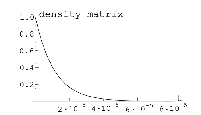
Figure 1: Density matrix $({\rho}^{0}_{\mathbf{p}~{}\mathbf{p}}(t))_{diag}:~{}m=0.51~{}MeV,~{}|\textbf{p}|=0~{}MeV,~{}\omega=12.8~{}eV$, t(sec.)

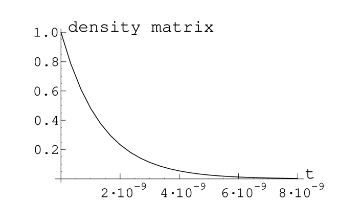
Figure 2: Density matrix $({\rho}^{0}_{\mathbf{p}~{}\mathbf{p}}(t))_{diag}:~{}m=0.51~{}MeV,~{}|\textbf{p}|=0.001~{}MeV,~{}\omega=12.8~{}eV$, t(sec.)

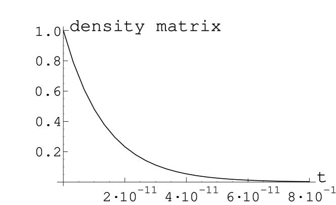
Figure 3: Density matrix $({\rho}^{0}_{\mathbf{p}~{}\mathbf{p}}(t))_{diag}:~{}m=0.51~{}MeV,~{}|\textbf{p}|=0.01~{}MeV,~{}\omega=12.8~{}eV$, t(sec.)

References

- [1] I. Prigogine, From Being to Becoming, Freeman, San Francisco, 1980.
- [2] I. Prigogine, I. Stengers, Order out of Chaos: Man’s New Dialogue with Nature, Boulder, C.O., New Science Library, 1984.
- [3] I. Prigogine, C. George and F. Henin, Physica (Amsterdam) 45, 418 (1969).
- [4] I. Prigogine, C. George, F. Henin and L. Rosenfeld, Chemica Scripta 4, 5 (1973).
- [5] B. Misra, I. Prigogine and M. Courbage, Physica A 98, 1 (1979).
- [6] T. Y. Petrosky and I. Prigogine, Physica A 147, 439 (1988).
- [7] I. Prigogine and T. Y. Petrosky, Physica A 147, 461 (1988).
- [8] T. Y. Petrosky and H. Hasegawa, Physica A 160, 351 (1989).
- [9] T. Y. Petrosky and I. Prigogine, Can. J. Phys. 68, 670 (1990).
- [10] T. Y. Petrosky, I. Prigogine and S. Tasaki, Physica A 173, 175 (1991).
- [11] T. Y. Petrosky and I. Prigogine, Physica A 175, 146 (1991).
- [12] I. Prigogine, Phys. Rep. 219, 93 (1992).
- [13] I. Antoniou and I. Prigogine, Nuovo Cimento 219, 93 (1992).
- [14] T. Petrosky and I. Prigogine, Phys. Lett. A 182, 1 (1993).
- [15] I. Antoniou and S. Tasaki, International J. of Quantum Chemistry 46, 425 (1993).
- [16] I. Antoniou and I. Prigogine, Physica A 192, 443 (1993).
- [17] T. Petrosky and I. Prigogine, Chaos, Solitons, Fractals 4, 311 (1994).
- [18] T. Petrosky and I. Prigogine, Chaos, Solitons, Fractals 7, 441 (1996).
- [19] I. Antoniou, Z. Suchanecki, R. Laura and S. Tasaki, Physica A 241, 737 (1997).
- [20] T. Petrosky and I. Prigogine, Adv. Chem. Phys. 99, 1 (1997).
- [21] I. Prigogine, Physica A 263, 528 (1999).
- [22] T. Petrosky and I. Prigogine, Chaos, Solitons, Fractals 11, 373 (2000).
- [23] C. George, F. Mayne and I. Prigogine, Adv. Chem. Phys. 61, 223 (1985).
- [24] T. Petrosky, G. Ordonez and T. Miyasaka, Phys. Rev. A 53, 4075 (1996).
- [25] G. Ordonez, T. Petrosky and I. Prigogine, Phys. Rev. A 63, 052106 (2001).
- [26] T. Petrosky, G. Ordonez and I. Prigogine, Phys. Rev. A 64, 062101 (2001).
- [27] E. Karpov, G. Ordonez, T. Petrosky and I. Prigogine, Phys. Rev. A 66, 012109 (2002).
- [28] I. Antoniou, M. Gadella, I. Prigogine and G. P. Pronko, J. of Math. Phys. 39, 2995 (1998).
- [29] I. Antoniou, M. Gadella and G. Pronko, Chaos, Solitons, Fractals 12, 2737 (2001).
- [30] I. Antoniou, M. Gadella, E. Karpov, I. Prigogine and G. Pronko, Chaos, Solitons, Fractals 12, 2757 (2001).
- [31] I. Antoniou, M. Gadella, J. Mateo and G.P. Pronko International J. of Theor. Phys. 42, 2389 (2003).
- [32] I. Antoniou, E. Karpov, G. Pronko and E. Yarevsky International J. of Theor. Phys. 42, 2403 (2003).
- [33] G. Ordonez, T. Petrosky, E. Karpov and I. Prigogine, Chaos, Solitons, Fractals 12, 2591 (2001).
- [34] T. Petrosky and G. Ordonez, Phys. Rev. A 56, 3507 (1997).
- [35] R. Passante, T. Petrosky and I. Prigogine, Physica A 218, 437 (1995).
- [36] M. Rosenberg and T. Petrosky, Chaos, Solitons, Fractals 34, 533 (1997).
- [37] E. Karpov, I. Prigogine, T. Petrosky and G. Pronko, J. of Math. Phys. 41, 118 (2000).
- [38] T. Petrosky, G. Ordonez and I. Prigogine, Phys. Rev. A 62, 042106 (2000).
- [39] I. Antoniou and Yu. Melnikov, Chaos, Solitons, Fractals 12, 2603 (2001).
- [40] E. Karpov, G. Ordonez, T. Petrosky and I. Prigogine, Physics of Particles and Nuclei, Letters 1[116], 8 (2003).
- [41] T. Petrosky, G. Ordonez and I. Prigogine, Phys. Rev. A 68, 022107 (2003).
- [42] T. Petrosky, C.O. Ting, and V. Barsegov, Chaos, Solitons, Fractals 16, 381 (2003).
- [43] I. Antoniou, E.Karpov and G. Pronko, Chaos, Solitons, Fractals 17, 277 (2003).
- [44] I. Antoniou, E. Karpov, G. Pronko and E. Yarevsky, Chaos, Solitons, Fractals 17, 311 (2003).
- [45] I. Antoniou, M. Gadella, J. Mateo and G. Pronko, J. Phys A: Math. Gen. 36, 12109 (2003).
- [46] G. Ordonez and S. Kim, Phys. Rev. A 70, 032702 (2004).
- [47] C. George, Physica (Amsterdam) 65, 277 (1973).
- [48] M. De Haan and F. Henin, Physica (Amsterdam) 67, 197 (1973).
- [49] A. Grecos, T. Guo and W. Guo, Physica A 80, 421 (1975).
- [50] S. Kim and G. Ordonez, arXiv: physics/0311048, (2003).
- [51] M. De Haan, C. George and F. Mayne, Physica A 92, 584 (1978).
- [52] M. De Haan, Annals of Phys. 314, 10 (2004).
- [53] M. De Haan, Annals of Phys. 321, 507 (2006).
- [54] C. Obcemea and E. Brandas, Annals of Phys. 151, 383 (1983).
- [55] C. Lockhart and B. Misra, Physica A 136, 47 (1986).
- [56] J. Kumicak and E. Brandas, International J. of Quantum Chemistry 32, 669 (1987).
- [57] H. H. Hasegawa and W. C. Saphir, Phys. Rev. A 46, 7401 (1992).
- [58] H. H. Hasegawa and D. Driebe, Phys. Rev. E 50, 1781 (1994).
- [59] S.M. Bilenky, An introduction to Feynman diagrammatic formalism, Moscow, Atomizdat, 1971.
- [60] S.S. Schweber, An introduction to relativistic quantum field theory, N.Y., Row, Peterson and Co Evanston, Ill., Elmsford, 1961.
- [61] I. Prigogine, NonEquilibrium Statistical Mechanics, Wiley Interscience, New York, 1962.
- [62] T. Petrosky and I. Prigogine, Adv. Chem. Phys. 99, 1 (1997).
- [63] C. George, Bull. Acad. Roy. Bel. 5, 505 (1970).
- [64] S. Eh. Shirmovsky, arXiv: nucl-th/0603017, (2006).