Linear Optics Quantum Computation: an Overview

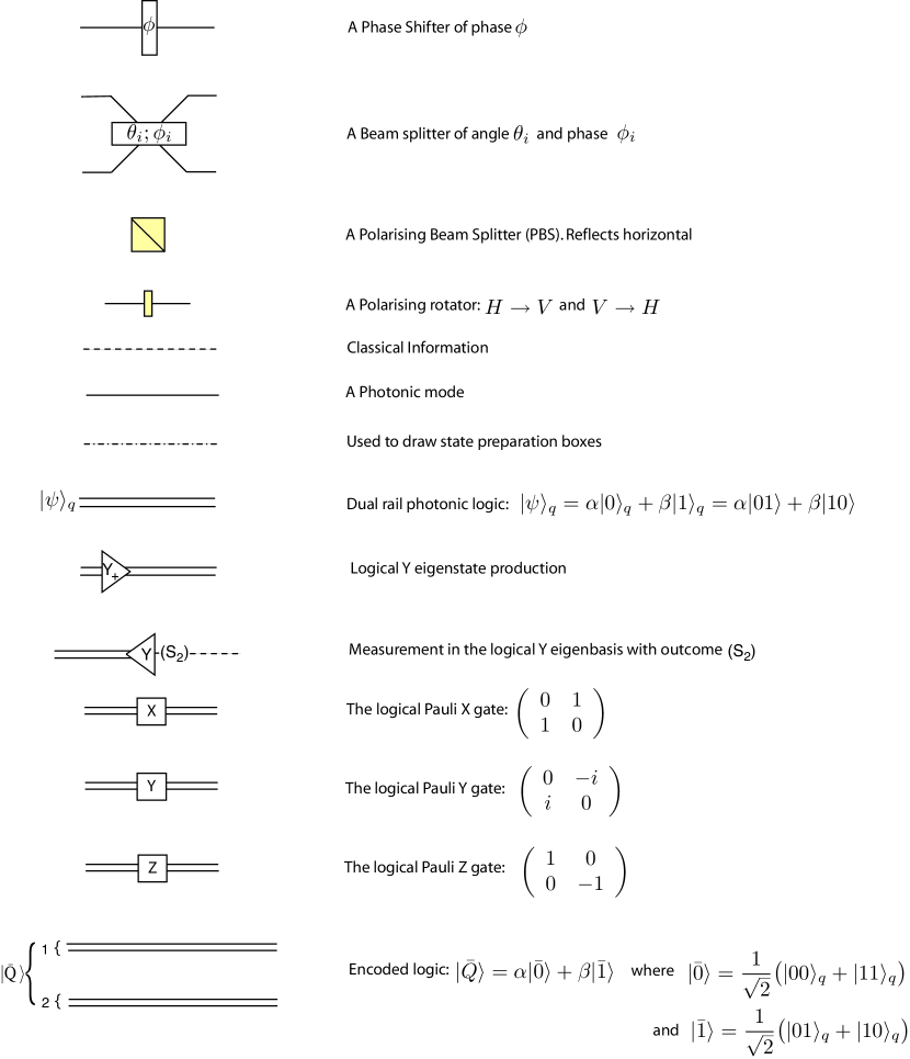
Figure 1: Notation for the lectures.

1 Quantum Information Processing with linear optics

There are at least three ways to understand these lectures on linear optics quantum computing:

• these are engineering lectures on how to build an optical quantum computer. We will give a step by step approach on how to use beam splitters, phase shifters, single photon sources and detectors to efficiently simulate an ideal quantum computer. In this sense, these lectures can really be thought of as being an engineering recipe,

• they can be thought of as lectures on quantum error correction. In order to use the simple elements mentioned above to build quantum information processing devices we will have to rely heavily on ideas and concepts of quantum error correction. By putting elements together and using detectors, a simple error model will emerge (projection of a qubit in the $Z$ basis) and we will use fault tolerant error correction to ensure that the quantum information is protected. We will even calculate a value for the accuracy threshold,

• or these can be seen as lectures on what quantum information is. These lecture will teach you that maybe we do not understand what quantum information really is. Some years ago it was thought that a quantum computation would be implemented by doing very precise unitary transformations. Here we will do very non-unitary operations (projections) on physical qubits but we will still be able to show that at a higher level this can mimic a unitary evolution efficiently. Linear optics will allow us to do a set of transformation that can be simulated efficiently by a classical computer. It is only when we condition our operations on the results of measurements that the system becomes hard to be simulated classically.

1.1 Quantum optics and quantum information

These lectures will be divided into three sections. First an introduction to quantum optics which will include some historical notes on the use of quantum optics for quantum information processing (QIP). The second section will focus on using linear optics with single photon sources and detectors (sometimes called the LOQC or KLM theory). The third section will focus on quantum error correction and LOQC.

1.2 Quantum Computation

Quantum information promises to solve some problems that have no known efficient classical algorithms. This is done by harnessing the size of Hilbert space and the ability to manipulate the quantum state.

David DiVincenzo [1] has suggested a set of five criteria that are sufficient for a device to be used as a quantum computer:

1. A scalable physical system with well characterised qubits.

2. The ability to initialise the state of the qubits to a simple fiducial state, such as $|{000\ldots}\rangle$.

3. A “universal” set of quantum gates such as generic one qubit gates and a two qubit gate,

4. A qubit-specific measurement capability.

5. Long relevant decoherence times, much longer than the gate operation time.

1.3 Why optics?

Many physical systems have be proposed for quantum computation. Each has its own advantages and disadvantages. For example, in an ion trap, two qubit gates are relatively easy to implement. However, isolating the ions from the environment is difficult, the ions’ motion being vulnerable to decoherence. In NMR quantum computing, the most successful proposal to date, nuclear spin states can be handled directly. However, the ability to initialise a simple fiducial state is difficult. Also, many nuclear spins must be present in order for a sizable signal to be observed.

The first proposal for quantum computing involved single photons as qubits [7]. One advantage for using single photons in QIP is that quantum optics is a well developed field. Photons decohere slowly, an ideal trait for quantum computing. Photons also travel well, one reason why they are so widely used for communication. Another advantage is that photons can be experimented with at room temperature.

One of the major obstacles for using single photons for QIP is that photons do not interact directly, making two qubit gates very difficult. Mode matching with single photon is also a problem. Another difficulty with using single photons is how to produce and detect them. To date the best single photon sources and detectors both have efficiencies well below any known threshold for scalable quantum computation.

1.4 Quantum Optics

1.4.1 Classical Electromagnetic Field

When we deal with electromagnetic waves classically we look for solutions to the source free Maxwell eqs.

$$\nabla^{2}{\bf E}({\bf r},t)-\frac{1}{c}\frac{\partial^{2}}{\partial t^{2}}{\bf E}({\bf r},t)=0$$ (1)

The solution have a plus and minus frequency part [2, 3] :

$${\bf E}({\bf r},t)=i\sum_{k}\biggl{(}\frac{\hbar\omega_{k}}{2}\biggr{)}^{\frac{1}{2}}[a_{k}{\bf u}_{k}({\bf r})e^{-i\omega_{k}t}+a^{*}_{k}{\bf u}^{*}_{k}({\bf r})e^{i\omega_{k}t}]$$ (2)

The ${\bf u}_{k}({\bf r})$ are orthogonal mode functions, usually plane wave mode functions ( ${\bf u}_{k}({\bf r})=\frac{\hat{{\bf e}}^{(\lambda)}}{\sqrt{V}}\exp(i{\bf k}\cdot{\bf r})$, where $\hat{{\bf e}}^{(\lambda)}$ is the unit polarisation vector and $V$ is the volume), and the $a_{k}$ are dimensionless (complex) amplitudes.

The energy of a classical electromagnetic field is given by

$$H=\frac{1}{2}\int_{V}({\bf E}^{2}+{\bf B}^{2})d{\bf r}=\sum_{k}\biggl{(}\frac{\hbar\omega_{k}}{2}\biggr{)}a_{k}a^{*}_{k}$$ (3)

1.4.2 Quantise

We quantise the electromagnetic field by turning the coefficient $a_{k}$ into operators and imposing the commutation relations:

$$[\hat{a}_{i},\hat{a}^{\dagger}_{j}]=\delta_{i,j}$$ (4)

$$[\hat{a}_{i},\hat{a}_{j}]=[\hat{a}^{\dagger}_{i},\hat{a}^{\dagger}_{j}]=0.$$ (5)

In terms of these operators the energy is given by

$$\hat{H}=\sum_{k}\hbar\omega_{k}\bigl{(}\hat{a}^{\dagger}_{k}\hat{a}_{k}+\frac{1}{2}\bigr{)}.$$ (6)

If we let

$$\hat{a}=\frac{1}{\sqrt{2}}\bigl{(}\sqrt{\frac{m\omega}{\hbar}}\hat{x}+i\frac{1}{\sqrt{m\hbar\omega}}\hat{p}\bigr{)}$$ (7)

the energy of the electromagnetic field becomes

$$\hat{H}=\frac{\hat{p}^{2}}{2m}+\frac{1}{2}m\omega^{2}\hat{x}^{2}$$

from which we can recognise the harmonic oscillator.

We call $\hat{a}$ an annihilation operator and $\hat{a}^{\dagger}$ a creation operator, the reason for this will be shown in eqs. (8) and (9).

The eigenstates of $\hat{H}$ are labeled $|{n}\rangle$ and we call them Fock states. We define the number operator $\hat{n}$ by $\hat{n}|{n}\rangle=\hat{a}^{\dagger}\hat{a}|{n}\rangle=n|{n}\rangle$.

What is the effect of $\hat{a}$ on $|{n}\rangle$? We can answer this by finding the number of photons in $\hat{a}|{n}\rangle$:

$$\hat{n}\bigl{(}\hat{a}|{n}\rangle\bigr{)}=\hat{a}^{\dagger}\hat{a}^{2}|{n}\rangle=\bigl{(}\hat{a}\hat{a}^{\dagger}\hat{a}-\hat{a}\bigr{)}|{n}\rangle=\bigl{(}n-1\bigr{)}\hat{a}|{n}\rangle$$

So $\hat{a}|{n}\rangle$ is a Fock state with $n-1$ photons. We define this to be $A|{n-1}\rangle$. In a similar way we can show that $\hat{a}^{\dagger}|{n}\rangle$ is a Fock state with $n+1$ photons, $B|{n+1}\rangle$. But what is the form of $A$ and $B$?

We can use the fact that $\langle{n}|\hat{n}|{n}\rangle=n$:

$$\langle{n}|\hat{n}|{n}\rangle = \langle{n}|\hat{a}^{\dagger}\hat{a}|{n}\rangle=A\langle{n}|\hat{a}^{\dagger}|{n-1}\rangle$$

$$= \langle{n-1}|A^{2}|{n-1}\rangle=A^{2}=n$$

$$\langle{n}|\hat{n}|{n}\rangle = \langle{n}|\hat{a}^{\dagger}\hat{a}|{n}\rangle=\langle{n}|\hat{a}\hat{a}^{\dagger}-1|{n-1}\rangle$$

$$= B^{2}-1=n$$

So we see that $\hat{a}$ acts as an annihilation operator and $\hat{a}^{\dagger}$ as a creation operator:

$$\hat{a}^{\dagger}|{n}\rangle = \sqrt{n+1}|{n+1}\rangle$$ (8)

$$\hat{a}|{n}\rangle = \sqrt{n}|{n-1}\rangle$$ (9)

from which we deduce that $n$ is a semi-positive number.

For $n=0$, $\hat{a}|{0}\rangle=0$ and $\hat{H}|{0}\rangle=\frac{1}{2}\hbar\omega|{0}\rangle$ representing vacuum fluctuation energy of the lowest eigenstate of the Hamiltonian.

The Fock states form an orthonormal set:

$$\langle n|m\rangle = \delta_{nm}$$

$$\sum_{n=0}^{\infty}|n\rangle\!\langle n| = {\mathchoice{\rm 1\mskip-4.0mul}{\rm 1\mskip-4.0mul}{\rm 1\mskip-4.5mul}{\rm 1\mskip-5.0mul}}$$

And each Fock state may be built up from creation operators:

$$|{n}\rangle=\frac{\bigl{(}\hat{a}^{\dagger}\bigr{)}^{n}}{\sqrt{n!}}|{0}\rangle$$ (10)

Exercise: show that $|{n}\rangle=\frac{\bigl{(}\hat{a}^{\dagger}\bigr{)}^{n}}{\sqrt{n!}}|{0}\rangle$. The matrix form of the annihilation operator can be seen by using the identity operator twice:

$$\hat{a} = {\mathchoice{\rm 1\mskip-4.0mul}{\rm 1\mskip-4.0mul}{\rm 1\mskip-4.5mul}{\rm 1\mskip-5.0mul}}\hat{a}{\mathchoice{\rm 1\mskip-4.0mul}{\rm 1\mskip-4.0mul}{\rm 1\mskip-4.5mul}{\rm 1\mskip-5.0mul}}=\sum_{n=0}^{\infty}|n\rangle\!\langle n|\hat{a}\sum_{m=0}^{\infty}|m\rangle\!\langle m|$$

$$= \sum_{n=0}^{\infty}\sqrt{n+1}|n\rangle\!\langle n+1|$$

In matrix form:

$$\hat{a}=\left(\begin{array}[]{ccccc}0&\sqrt{1}&0&0&\cdots\\ 0&0&\sqrt{2}&0&\cdots\\ 0&0&0&\sqrt{3}&\cdots\\ \vdots&\vdots&\vdots&\vdots&\ddots\\ \end{array}\right)$$

In eq. (7) we wrote $\hat{a}$ in terms of $\hat{x}$ and $\hat{p}$. It is often more convenient to write the annihilation operator as a linear combination of the two Hermitian operators:

$$\hat{a}=\frac{\hat{Q}_{1}+i\hat{Q}_{2}}{2}$$

where $\hat{Q}_{1}$ (equivalent to $\hat{x}$ from before) corresponds to the in-phase component of the electric field amplitude of the spatial-temporal mode and $\hat{Q}_{2}$ (equivalent to $\hat{p}$ from before) corresponds to the out-of-phase component.

This gives the commutation relation $[\hat{Q}_{1},\hat{Q}_{2}]=2i$ and the Heisenberg uncertainty relation

$$\Delta\hat{Q}_{1}\Delta\hat{Q}_{2}\geq 1$$

With the annihilation and creation operators defined in this way it is instructive to look at the position and momentum wave functions for Fock states. First note that $\psi(Q_{1})=\langle Q_{1}|\psi\rangle$ and $\tilde{\psi}(Q_{2})=\langle Q_{2}|\psi\rangle$, where we know that $\hat{Q_{1}}|{Q_{1}}\rangle=Q_{1}|{Q_{1}}\rangle$ and $\hat{Q_{2}}|{Q_{2}}\rangle=Q_{2}|{Q_{2}}\rangle$. Also note the usual normalisation rules: $\langle Q_{1}|Q_{1}^{{}^{\prime}}\rangle=\delta(Q_{1}-Q_{1}^{{}^{\prime}})$ and $\langle Q_{2}|Q_{2}^{{}^{\prime}}\rangle=\delta(Q_{2}-Q_{2}^{{}^{\prime}})$, $\delta(x-x^{{}^{\prime}})$ being the Dirac Delta function.

When we look at the position and momentum wave functions for the vacuum state we have [4]

$$\langle Q_{1}|0\rangle = \psi_{0}(Q_{1})=\pi^{-\frac{1}{4}}\exp\bigl{(}-\frac{Q_{1}^{2}}{4}\bigr{)}$$

$$\langle Q_{2}|0\rangle = \tilde{\psi}_{0}(Q_{2})=\pi^{-\frac{1}{4}}\exp\bigl{(}-\frac{Q_{2}^{2}}{4}\bigr{)}$$

And in general for a Fock state $|{n}\rangle$ we have

$$\langle Q_{1}|n\rangle=\psi_{n}(Q_{1})=\frac{H_{n}(\frac{Q_{1}}{\sqrt{2}})}{\sqrt{2^{n}n!}\sqrt{\pi}}\exp\bigl{(}-\frac{Q_{1}^{2}}{4}\bigr{)}$$

where $H_{n}(x)$ is the Hermite polynomials.

1.4.3 Minimum Uncertainty States

The Heisenberg Uncertainty Principle: for two non-commuting observables $\hat{A}$ and $\hat{B}$, the uncertainty in each is given by the relation:

$$\Delta\hat{A}\Delta\hat{B}\geq\frac{1}{2}|<[\hat{A},\hat{B}]>|$$

where $(\Delta\hat{A})^{2}=\langle\hat{A}^{2}\rangle-\langle\hat{A}\rangle^{2}$.

For example, consider the case when $\hat{A}=\hat{x}$ and $\hat{B}=\hat{p}$. The uncertainty principle becomes the well known result: $\Delta\hat{x}\Delta\hat{p}\geq\frac{\hbar}{2}$

A coherent state $|{\alpha}\rangle$ is a minimum uncertainty state. We can define it as the eigenstate of an annihilation operator: $\hat{a}|{\alpha}\rangle=\alpha|{\alpha}\rangle$ Alternatively, we can define it with the displacement operator $D(\alpha)$:

$$|{\alpha}\rangle = D(\alpha)|{0}\rangle=\exp(\alpha\hat{a}^{\dagger}-\alpha^{*}\hat{a})|{0}\rangle$$

$$= \exp(-\frac{|\alpha|^{2}}{2})\exp(\alpha\hat{a}^{\dagger})|{0}\rangle$$

Exercise: show the last line for the above coherent state definition is correct using the Campbell-Baker-Hausdorff operator identity:

$$e^{\hat{A}+\hat{B}}=e^{\hat{A}}e^{\hat{B}}e^{-\frac{1}{2}[\hat{A},\hat{B}]}$$

for the case when $[\hat{A},[\hat{A},\hat{B}]]=[\hat{B},[\hat{A},\hat{B}]]=0$.

Exercise: show that $\hat{a}D(\alpha)|{0}\rangle=\alpha D(\alpha)|{0}\rangle$.

If we work out $\Delta\hat{Q_{1}}\Delta\hat{Q_{2}}$ for a coherent state we find that $\Delta\hat{Q_{1}}=\Delta\hat{Q_{2}}=1$, showing that coherent states are minimum uncertainty states, since $\Delta\hat{Q_{1}}\Delta\hat{Q_{2}}=1$.

Coherent states are not orthogonal since

$$\langle\beta|\alpha\rangle=\exp[-\frac{1}{2}\bigl{(}|\alpha|^{2}+|\beta|^{2}\bigr{)}+\alpha\beta^{*}]$$

and as such form an over complete set

$$\int|\alpha\rangle\!\langle\alpha|d^{2}\alpha=\pi$$

If we look at the wave functions for a coherent state ($\langle Q_{1}|\alpha\rangle=\psi_{\alpha}(Q_{1})$ and $\langle Q_{2}|\alpha\rangle=\tilde{\psi}_{\alpha}(Q_{2})$) [4] we find that

$$\psi_{\alpha}(Q_{1}) = \pi^{-\frac{1}{4}}\exp\Bigl{(}-\frac{(Q_{1}-q_{0})^{2}}{4}+\frac{i}{4}p_{0}Q_{1}-\frac{i}{8}p_{0}q_{0}\Bigr{)}$$

$$\tilde{\psi}_{\alpha}(Q_{2}) = \pi^{-\frac{1}{4}}\exp\Bigl{(}-\frac{(Q_{2}-p_{0})^{2}}{4}-\frac{i}{4}q_{0}Q_{2}+\frac{i}{8}p_{0}q_{0}\Bigr{)}$$

where we have decomposed the complex amplitude $\alpha$ into its real and imaginary parts: $\alpha=\frac{1}{2}\bigl{(}q_{0}+ip_{0}\bigr{)}$. From this we see that a coherent state is a Gaussian in $Q_{1},Q_{2}$ phase space.

Squeezed states are another type of minimum uncertainty state. Squeezed state have one of $\Delta\hat{Q_{1}}$ or $\Delta\hat{Q_{2}}$ “squeezed” below 1 at the expense of the other: either $\Delta\hat{Q_{1}}<1<\Delta\hat{Q_{2}}$ or $\Delta\hat{Q_{2}}<1<\Delta\hat{Q_{1}}$ such that $\Delta\hat{Q_{1}}\Delta\hat{Q_{2}}=1$ is always true.

We can define squeezed states with the Squeeze operator

$$S(\epsilon)=\exp{\Bigl{(}\frac{1}{2}\epsilon^{*}\hat{a}^{2}-\frac{1}{2}\epsilon\bigl{(}\hat{a}^{\dagger}\bigr{)}^{2}\Bigr{)}}$$

where $\epsilon=re^{i\varphi}$.

If we define a rotated complex plane: $\hat{P_{1}}+i\hat{P_{2}}=\bigl{(}\hat{Q_{1}}+i\hat{Q_{2}}\bigr{)}e^{-\frac{i}{2}\varphi}$ then the uncertainties can be written as $\Delta\hat{P_{1}}=e^{-r}$ and $\Delta\hat{P_{2}}=e^{r}$. Squeezed coherent states are defined to be $|{\alpha,\epsilon}\rangle=D(\alpha)S(\epsilon)|{0}\rangle$.

If we look at the wave functions for a squeezed coherent state [4] we see that $\langle{Q_{1}}|D(\alpha)S(\epsilon)|{0}\rangle$:

$$\pi^{-\frac{1}{4}}e^{\frac{\epsilon}{2}}\exp\Bigl{(}-e^{2\epsilon}\frac{(Q_{1}-q_{0})^{2}}{4}+\frac{i}{4}Q_{2}Q_{1}-\frac{i}{8}p_{0}q_{0}\Bigr{)}$$

where we have again decomposed the complex amplitude $\alpha$ into its real and imaginary parts: $\alpha=\frac{1}{2}\bigl{(}q_{0}+ip_{0}\bigr{)}$. As with the coherent state, we see that a squeezed coherent state is a Gaussian in $Q_{1},Q_{2}$ phase space.

1.5 Linear Optics

What does “Linear Optics” mean?

An optical component is said to be linear if its output modes $\hat{b}^{\dagger}_{j}$ are a linear combination of its input modes $\hat{a}^{\dagger}_{j}$:

$$\hat{b}^{\dagger}_{j}=\sum_{k}M_{jk}\hat{a}^{\dagger}_{k}$$

Linear optical components are made up of phase shifters and beam splitters. A phase shifter is defined by the transformation $U(P_{\phi}):|{n}\rangle\to e^{in\phi}|{n}\rangle$. That is, $\bigl{(}\hat{a}_{l}^{\dagger}\bigr{)}^{n}|{0}\rangle\to e^{in\phi}\bigl{(}\hat{a}_{l}^{\dagger}\bigr{)}^{n}|{0}\rangle$.

The Hamiltonian for a phase shifter is given by the number operator: $U=e^{i\phi\hat{H}}=e^{i\phi\hat{n}}=e^{i\phi\hat{a}^{\dagger}\hat{a}}$. Using this see we that $e^{i\phi\hat{a}^{\dagger}\hat{a}}|{n}\rangle=e^{in\phi}|{n}\rangle$ Exercise: show that the phase operator takes a coherent state $|{\alpha}\rangle$ to $|{e^{i\phi}\alpha}\rangle$.

A beam splitter is defined by the transformation matrix

$$U=\left(\begin{array}[]{cc}\cos\theta&-e^{i\phi}\sin\theta\\ e^{-i\phi}\sin\theta&\cos\theta\end{array}\right)$$ (14)

where the input modes are related to the output modes via $a^{\dagger}_{l}|{0}\rangle\rightarrow\sum_{m}U_{ml}a^{\dagger}_{m}|{0}\rangle$ Exercise: The Hamiltonian for a beam splitter can be given by $\hat{H}=e^{i\phi}\hat{a}^{\dagger}\hat{b}+e^{-i\phi}\hat{a}\hat{b}^{\dagger}$, check that this is Hermitian.

The unitary transformation for a beam splitter then looks like $\exp\Bigl{(}-i\theta\bigl{(}e^{i\phi}\hat{a}_{k}^{\dagger}\hat{a}_{l}+e^{-i\phi}\hat{a}_{k}\hat{a}_{l}^{\dagger}\bigr{)}\Bigr{)}$, where $k$ and $l$ are the two modes being acted upon by the beam splitter.

Consider we have the state $|{mn}\rangle_{12}$ incident on a beam splitter. The output would look like:

$$|{mn}\rangle_{12}=\frac{\bigl{(}\hat{a}_{1}^{\dagger}\bigr{)}^{m}}{\sqrt{m!}}\frac{\bigl{(}\hat{a}_{2}^{\dagger}\bigr{)}^{n}}{\sqrt{n!}}|{00}\rangle \to \frac{1}{\sqrt{m!}}\Bigl{(}\sum_{i}U_{i1}\hat{a}_{i}^{\dagger}\Bigr{)}^{m}\frac{1}{\sqrt{n!}}\Bigl{(}\sum_{i}U_{j2}\hat{a}_{j}^{\dagger}\Bigr{)}^{n}|{00}\rangle$$

$$= \frac{1}{\sqrt{m!n!}}\Bigl{(}\hat{a}_{1}^{\dagger}\cos\theta+\hat{a}_{2}^{\dagger}e^{-i\phi}\sin\theta\Bigr{)}^{m}\Bigl{(}\hat{a}_{1}^{\dagger}e^{-i\phi}\sin\theta+\hat{a}_{2}^{\dagger}\cos\theta\Bigr{)}^{n}|{00}\rangle$$

For example:

$$|{10}\rangle \rightarrow\cos\theta|{10}\rangle+e^{-i\phi}\sin\theta|{01}\rangle$$

$$|{01}\rangle \rightarrow-e^{i\phi}\sin\theta|{10}\rangle+\cos\theta|{01}\rangle$$

$$|{11}\rangle \rightarrow-\sqrt{2}e^{i\phi}\cos\theta\sin\theta|{20}\rangle+(\cos^{2}\theta-\sin^{2}\theta)|{11}\rangle$$

$$\hskip 28.45274pt+\sqrt{2}e^{-i\phi}\cos\theta\sin\theta|{02}\rangle$$

$$|{20}\rangle \rightarrow\cos^{2}\theta|{20}\rangle+\sqrt{2}e^{-i\phi}\cos\theta\sin\theta|{11}\rangle+e^{-2i\phi}\sin^{2}\theta|{02}\rangle$$

$$|{02}\rangle \rightarrow e^{2i\phi}\sin^{2}\theta|{20}\rangle-\sqrt{2}e^{i\phi}\cos\theta\sin\theta|{11}\rangle+\cos^{2}\theta|{02}\rangle$$

Exercise: confirm these examples.

1.6 Previous Suggestions With Optics

Photons are an ideal means for communication, they travel fast and only interact weakly with their surrounding and thus have a long decoherence time. The problem with using solely optics for quantum computation is how to get photons to interact. It is relatively easy to achieve single qubit gates, but how do we establish two qubit gates? This isn’t the only problem, we also have to achieve two qubit gates that are efficient in resources so our system will be scalable. One way to make photons interact is to induce a cross phase modulation between two optical modes. One example of this is the Kerr effect.

1.6.1 Quantum Optical Fredkin Gate

The first proposal for quantum computation was the quantum optical Fredkin gate [6, 7]. The gate was realised with single photon optics using the Kerr Effect. A Fredkin gate is a three qubit gate that acts as a controlled swap. Its truth table is given below.

$c_{i}$	$a_{i}$	$b_{i}$	$c_{o}$	$a_{o}$	$b_{o}$
0	0	0	0	0	0
0	0	1	0	0	1
0	1	0	0	1	0
0	1	1	0	1	1
1	0	0	1	0	0
1	0	1	1	1	0
1	1	0	1	0	1
1	1	1	1	1	1

Table 1: The logic for a Fredkin gate. Here subscript $i$ refers to the input qubits, $o$ refers to the output qubits and $c$ is the control qubit.

In this scheme, logical 0 corresponds to the vacuum mode $|{0}\rangle$ and logical 1 is the 1 photon Fock state $|{1}\rangle$.

The optical Kerr effect is defined by a material with an intensity dependent refractive index, that is, a nonlinear crystal that has an index of refraction $n$ proportional to the total intensity $I$: $n=n_{0}+n_{2}E^{2}=n_{0}+n_{2}I$, where $n_{0}$ is the normal refractive index and $n_{2}$ is the correction term necessary for Kerr materials.

The Kerr Hamiltonian is of the form

$$H_{I}=-\hbar\chi\hat{a}^{\dagger}_{1}\hat{a}_{1}\hat{a}^{\dagger}_{2}\hat{a}_{2}$$

where $\chi$ is a coupling constant which depends upon the third-order non-linear susceptibility for the optical Kerr effect and $\hat{a}_{1}$ and $\hat{a}_{2}$ are the annihilation modes for the input light.

The optical setup for the Fredkin gate first proposed in [7] is shown below in fig. 2. In this setup we have a Mach-Zehnder interferometer with a Kerr media in either arm. In the top arm the Kerr media has the control beam incident on it.

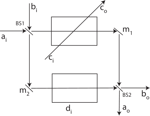
Figure 2: The original quantum Fredkin gate [7].

The beam splitter on the left side, BS1, has $\theta=\frac{\pi}{4},\phi=0$ and the beam splitter on the right hand side, BS2, has $\theta=\frac{\pi}{4},\phi=\pi$. The effect of the Kerr media is to act the unitary operator $U=\exp{\bigl{(}-i\frac{t}{\hbar}H_{I}\bigr{)}}=\exp{\bigl{(}i\epsilon\hat{a}^{\dagger}\hat{a}\hat{c}^{\dagger}\hat{c}\bigr{)}}$ in the top arm and $U=\exp{\bigl{(}i\epsilon\hat{b}^{\dagger}\hat{b}\hat{d}^{\dagger}\hat{d}\bigr{)}}$ in the bottom arm, where $\epsilon=t\chi$.

For example, consider the input state $|{cab,d}\rangle=|{010,0}\rangle$

$$|{010,0}\rangle \rightarrow\frac{1}{\sqrt{2}}\bigl{(}|{010,0}\rangle+|{001,0}\rangle\bigr{)}$$

$$\rightarrow\frac{1}{\sqrt{2}}e^{i\epsilon\hat{c}^{\dagger}\hat{c}\hat{a}^{\dagger}\hat{a}}e^{i\epsilon\hat{b}^{\dagger}\hat{b}\hat{d}^{\dagger}\hat{d}}\bigl{(}|{010,0}\rangle+|{001,0}\rangle\bigr{)}$$

$$=\frac{1}{\sqrt{2}}\bigl{(}e^{i\epsilon\hat{c}^{\dagger}\hat{c}\hat{a}^{\dagger}\hat{a}}|{010,0}\rangle+e^{i\epsilon\hat{b}^{\dagger}\hat{b}\hat{d}^{\dagger}\hat{d}}|{001,0}\rangle\bigr{)}$$

$$=\frac{1}{\sqrt{2}}\bigl{(}|{010,0}\rangle+|{001,0}\rangle\bigr{)}\rightarrow|{010,0}\rangle$$

where mode $d$ is always in the vacuum mode $|{0}\rangle$ and remember that $e^{i\phi\hat{n}}|{m}\rangle=e^{im\phi}|{m}\rangle$.

Next consider the input $|{101,0}\rangle$

$$|{101,0}\rangle \rightarrow\frac{1}{\sqrt{2}}\bigl{(}|{101,0}\rangle-|{110,0}\rangle\bigr{)}$$

$$\rightarrow\frac{1}{\sqrt{2}}\bigl{(}-e^{i\epsilon\hat{c}^{\dagger}\hat{c}\hat{a}^{\dagger}\hat{a}}|{110,0}\rangle+e^{i\epsilon\hat{b}^{\dagger}\hat{b}\hat{d}^{\dagger}\hat{d}}|{101,0}\rangle\bigr{)}$$

$$\rightarrow\frac{1}{\sqrt{2}}\bigl{(}-e^{i\epsilon}|{110,0}\rangle+|{101,0}\rangle\bigr{)}$$

$$\rightarrow\frac{1}{2}\bigl{(}-e^{i\epsilon}|{110,0}\rangle+e^{i\epsilon}|{101,0}\rangle+|{101,0}\rangle+|{110,0}\rangle\bigr{)}.$$

If we choose $\epsilon=\pi$ this gives $|{110,0}\rangle$. With this choice of $\epsilon$ we can show that all the logic gates are as in the Fredkin gate logic table.

There are two major problems with this scheme: (1) it is difficult to achieve the high non-linearities, especially those required for $\epsilon=\pi$ phase change; (2) at high non-linearities the crystal exhibits other detrimental affects, such as absorption.

1.6.2 Cavity Quantum Electrodynamics

Using non-linear crystals is not the only method to induce a coupling between optical modes. In [8] Turchette et. al. used cavity quantum electrodynamics to induce a two qubit interaction between photons. To do this single atoms in a Fabry-Perot cavity were used.

We start with the Jaynes-Cummings Hamiltonian for the interaction of photons with a two level atom:

$$H=\frac{1}{2}\hbar\omega_{0}(-Z)+\hbar\omega\hat{a}^{\dagger}\hat{a}+g\bigl{(}\hat{a}^{\dagger}\sigma_{-}+\hat{a}\sigma_{+}\bigr{)}$$ (15)

where $\omega_{0}$ is the frequency of the atom, $\omega$ the frequency of the field and $g$ is the coupling constant between the field and atom.

The first term in the above Hamiltonian is the atom energy term $H_{\text{atom}}=-\frac{1}{2}\hbar\omega_{0}Z$. We have a two level atom and we say the energy of the top level ($|{1}\rangle$) is $\frac{1}{2}\hbar\omega_{0}$ and that of the bottom level $|{0}\rangle$ is $-\frac{1}{2}\hbar\omega_{0}$. From the difference in energy we have $H_{\text{atom}}=\frac{1}{2}\hbar\omega_{0}\bigl{(}|1\rangle\!\langle 1|-|0\rangle\!\langle 0|\bigr{)}=-\frac{1}{2}\hbar\omega_{0}Z$, given that $Z=-(|1\rangle\!\langle 1|-|0\rangle\!\langle 0|)$. The $H_{\text{field}}=\hbar\omega\hat{a}^{\dagger}\hat{a}$ term comes from the harmonic oscillator describing light (and we have dropped the $\frac{1}{2}\hbar\omega$ term as it plays no role here) Finally, there is the interaction term $H_{I}$ which shows that an atom in the state $|{1}\rangle$ can decay to give a photon, or a photon can excite the atom from a state $|{0}\rangle$. $\sigma_{\pm}$ are the usual raising and lowering operators, $\sigma_{+}=|1\rangle\!\langle 0|=\frac{1}{2}\bigl{(}X+iY\bigr{)}$, $\sigma_{-}=|0\rangle\!\langle 1|=\frac{1}{2}\bigl{(}X-iY\bigr{)}$. The terms $\hat{a}^{\dagger}\sigma_{+}$ or $\hat{a}\sigma_{-}$ are dropped from this Hamiltonian by the so called rotating wave approximation.

We can rewrite the Jaynes-Cummings Hamiltonian in the following form, as done in [5]

$$H=\hbar\omega N+\delta Z+g\bigl{(}\hat{a}^{\dagger}\sigma_{-}+\hat{a}\sigma_{+}\bigr{)}$$ (16)

where $N=\hat{a}^{\dagger}\hat{a}+\frac{1}{2}Z$ and $\delta=\frac{1}{2}\hbar\bigl{(}\omega_{0}-\omega\bigr{)}$. We may neglect $N$ from any further analysis as it leads to a constant phase factor that we can neglect. We thus have a Hamiltonian that is reduced to:

$$H=\delta Z+g\bigl{(}\hat{a}^{\dagger}\sigma_{-}+\hat{a}\sigma_{+}\bigr{)}$$ (17)

The goal is to utilise a single atom to obtain a non-linear interaction between two photons. The quantum information will be represented by orthogonal polarisation photon states, using a cavity with a single atom to provide the non-linear interaction between the photons. We can modify the Hamiltonian (17) to incorporate two photons of slightly different frequencies and take photon polarisation into account. A three level atom that is excited to a different energy level (of approximately the same energy) by the two orthogonal polarisation, a so called $V$ type atom, suffices for this.

Turchette at. al. used Cesium atoms and two photons, one circularly polarised (mode $a$) and the other of slightly different frequency also circularly polarised (mode $b$), both generated from weak laser pulses. The logic was represented by the two orthogonal polarisation modes $|{1^{\pm}}\rangle_{a}|{1^{\pm}}\rangle_{b}$. The phases induced by interaction with the atom were then measured using heterodyne measurement.

The following logical transformations were measured:

$$|{1^{-}}\rangle_{a}|{1^{-}}\rangle_{b} \to |{1^{-}}\rangle_{a}|{1^{-}}\rangle_{b}$$

$$|{1^{+}}\rangle_{a}|{1^{-}}\rangle_{b} \to e^{i\phi_{a}}|{1^{+}}\rangle_{a}|{1^{-}}\rangle_{b}$$

$$|{1^{-}}\rangle_{a}|{1^{+}}\rangle_{b} \to e^{i\phi_{b}}|{1^{-}}\rangle_{a}|{1^{+}}\rangle_{b}$$

$$|{1^{+}}\rangle_{a}|{1^{+}}\rangle_{b} \to e^{i(\phi_{a}+\phi_{b}+\Delta)}|{1^{+}}\rangle_{a}|{1^{+}}\rangle_{b}$$

where $\phi_{a}\approx(17.5\pm 1)^{o}$, $\phi_{b}\approx(12.5\pm 1)^{o}$ and $\Delta\approx(16\pm 3)^{o}$.

The beauty of this interaction is that $|{1^{+}1^{+}}\rangle$ goes to $e^{\bigl{(}\varphi_{a}+\varphi_{b}+\Delta\bigr{)}}|{1^{+}1^{+}}\rangle$, where intuitively one might expect that $|{1^{+}1^{+}}\rangle$ would go to $e^{\bigl{(}\varphi_{a}+\varphi_{b}\bigr{)}}|{1^{+}1^{+}}\rangle$. This is the photon non-linearity. If $\Delta$ were 0, the system would be linear and the photons would not interact. This is the key for implementing quantum logic with these methods. Unfortunately it is much harder to get higher non linearities such as $\Delta=90^{o}$ and does not appears to be a promising approach when compounding many gates.

1.7 Progress with Linear Optics

Another direction to devise quantum information processor is to focus on linear optics alone. In this section we show what progress was made in this direction before the proposal by Knill et. al. [9].

1.7.1 Decomposition of unitaries

Reck et. al. showed that we can break any unitary into a set of linear optical components [10]. The unitary transformation considered is acting on the creation operators, so one is not able to immediately apply this method to say to the CNOT unitary.

A unitary operator $U$ of dimension $N$ can be decomposed as follows:

$$U=\Bigl{(}T_{N,N-1}\cdot T_{N,N-2}\cdot T_{N,N-3}\cdots T_{N,1}\cdot T_{N-1,N-2}\cdot T_{N-1,N-3}\cdots T_{2,1}D\Bigr{)}^{-1}$$ (18)

where $T_{p,q}$ is the $N$ dimensional identity with the $\{p,q\}$ elements replaced with the beam splitter matrix (14) and $D$ is an $N\times N$ matrix with phases on the diagonal.

The general linear optical network for a unitary matrix $U$ is a triangular array of beam splitters and phase shifters, shown in fig. 3.

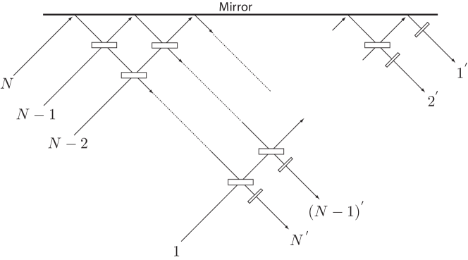
Figure 3: General linear optical network for a unitary matrix $U$.

As an example, what does the linear optical circuit for the following unitary look like?

$$U=\left(\begin{array}[]{ccc}1-\sqrt{2}&\frac{1}{\sqrt{\sqrt{2}}}&\sqrt{\frac{3}{\sqrt{2}}-2}\\ \frac{1}{\sqrt{\sqrt{2}}}&\frac{1}{2}&\frac{1}{2}-\frac{1}{\sqrt{2}}\\ \sqrt{\frac{3}{\sqrt{2}}-2}&\frac{1}{2}-\frac{1}{\sqrt{2}}&\sqrt{2}-\frac{1}{2}\\ \end{array}\right)$$

Exercise: check that this is unitary.

Here we have a unitary matrix with N=3, so we can say that

$$U=\Bigl{(}T_{3,2}\cdot T_{3,1}\cdot T_{2,1}\cdot D\Bigr{)}^{-1}=D^{\dagger}\cdot T_{2,1}^{\dagger}\cdot T_{3,1}^{\dagger}\cdot T_{3,2}^{\dagger}$$

We find that

$$T_{3,2}=\left(\begin{array}[]{ccc}1&0&0\\ 0&\cos\theta_{1}&e^{-i\phi_{1}}\sin\theta_{1}\\ 0&-e^{i\phi_{1}}\sin\theta_{1}&\cos\theta_{1}\\ \end{array}\right)$$

$$T_{3,1}=\left(\begin{array}[]{ccc}\cos\theta_{2}&0&e^{-i\phi_{2}}\sin\theta_{2}\\ 0&1&0\\ -e^{i\phi_{2}}\sin\theta_{2}&0&\cos\theta_{2}\\ \end{array}\right)$$

$$T_{2,1}=\left(\begin{array}[]{ccc}\cos\theta_{3}&e^{-i\phi_{3}}\sin\theta_{3}&0\\ -e^{i\phi_{3}}\sin\theta_{3}&\cos\theta_{3}&0\\ 0&0&1\\ \end{array}\right)$$

and

$$D=\left(\begin{array}[]{ccc}e^{i\phi_{4}}&0&0\\ 0&e^{i\phi_{5}}&0\\ 0&0&e^{i\phi_{6}}\\ \end{array}\right)$$

Exercise: show that a solution to this is given by the angles: $\theta_{1}=12.8^{o},\phi_{1}=\pi$, $\theta_{2}=20.4^{o},\phi_{2}=0$, $\theta_{3}=63.8,\phi_{3}=0$, $\phi_{4}=\pi,\phi_{5}=0,\phi_{6}=0$.

Exercise: What transformation does this implement on the input state $\bigl{(}\alpha|{0}\rangle+\beta|{1}\rangle+\gamma|{2}\rangle\bigr{)}|{10}\rangle$? What is the transformation if we measure $|{10}\rangle$ in modes 2 and 3? This will be important later!

1.7.2 Optical Simulation of Quantum Logic

In [11], Cerf et. al. proposed a scheme for quantum logic with only linear optical devices and a single photon. To simulate $n$ qubits a single photon is put into $2^{n}$ different paths.

A $\sqrt{\text{NOT}}$ gate is given by a beam splitter with $\theta=\frac{\pi}{4}$ and $\phi=-\frac{\pi}{2}$, where

$$\sqrt{\text{NOT}}=\frac{1}{\sqrt{2}}\left(\begin{array}[]{cc}1&i\\ i&1\\ \end{array}\right)$$

$$|{0}\rangle_{q}=|{01}\rangle \to \frac{1}{\sqrt{2}}\bigl{(}i|{10}\rangle+|{01}\rangle\bigr{)}$$

$$|{1}\rangle_{q}=|{10}\rangle \to \frac{1}{\sqrt{2}}\bigl{(}|{10}\rangle+i|{01}\rangle\bigr{)}$$

Three simple gate implementations proposed by Cerf et. al. are given in fig. 4.

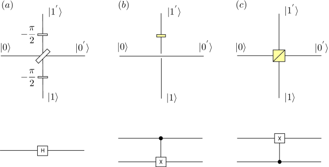
Figure 4: A Hadamard, a CNOT and a reverse CNOT.

With these a universal set of gates is possible.

To implement a Hadamard gate we use a $\theta=\frac{\pi}{4},\phi=-\frac{\pi}{2}$ beam splitter and two $-\frac{\pi}{2}$ phase shifters, as in part (a) of fig. 4.

$$|{0}\rangle_{q} = |{01}\rangle\rightarrow-i|{01}\rangle\rightarrow-\frac{i}{\sqrt{2}}\bigl{(}|{01}\rangle+i|{10}\rangle\bigr{)}$$

$$\rightarrow\frac{-i}{\sqrt{2}}\bigl{(}|{01}\rangle+i(-i)|{10}\rangle\bigr{)}=\frac{-i}{\sqrt{2}}\bigl{(}|{01}\rangle+|{10}\rangle\bigr{)}$$

$$|{1}\rangle_{q} = |{10}\rangle\rightarrow|{10}\rangle\rightarrow\frac{1}{\sqrt{2}}\bigl{(}i|{01}\rangle+|{10}\rangle\bigr{)}$$

$$\rightarrow\frac{1}{\sqrt{2}}\bigl{(}i|{01}\rangle+-i|{10}\rangle\bigr{)}=\frac{i}{\sqrt{2}}\bigl{(}|{01}\rangle-|{10}\rangle\bigr{)}$$

To implement a CNOT we encode a qubit in position and polarisation. The location is the control and the polarisation the target. For the control: $|{0}\rangle_{q}=|{01}\rangle$, $|{1}\rangle_{q}=|{10}\rangle$. For the target: $|{0}\rangle_{q}=|{H}\rangle$, $|{1}\rangle_{q}=|{V}\rangle$. The circuit for this is a polarisation rotator on the upper arm, as in part (b) of fig. 4. If a photon is present in the top arm, its polarisation will be flipped:

$$\bigl{(} \alpha|{01}\rangle+\beta|{10}\rangle\bigr{)}\otimes\bigl{(}\gamma|{H}\rangle+\delta|{V}\rangle\bigr{)}$$

$$\rightarrow\alpha\gamma|{01}\rangle|{H}\rangle+\alpha\delta|{01}\rangle|{V}\rangle+\beta\gamma|{10}\rangle|{V}\rangle+\beta\delta|{10}\rangle|{H}\rangle$$

To implement a reverse CNOT we simply need a polarising beam splitter (PBS), where horizontal is reflected. As before, the location is the control and the polarisation the target. This is in part (c) of fig. 4:

$$\bigl{(} \alpha|{01}\rangle+\beta|{10}\rangle\bigr{)}\otimes\bigl{(}\gamma|{H}\rangle+\delta|{V}\rangle\bigr{)}$$

$$\rightarrow\alpha\gamma|{01}\rangle|{H}\rangle+\alpha\delta|{10}\rangle|{V}\rangle+\beta\gamma|{10}\rangle|{H}\rangle+\beta\delta|{01}\rangle|{V}\rangle$$

The problem with this scheme is that $n$ qubits requires $2^{n}$ paths which in turn requires $2^{n}-1$ beam splitters to setup. This is not scalable. With one qubit encoded in polarisation we still need $2^{n-1}$ optical paths.

2 Linear Optics Quantum Compution

In this section we will develop ideas and concepts for linear optics quantum computing. We will show that using beam splitters, phase shifters, single photon sources and detectors we will be able to simulate efficiently, i.e. using a polynomial amount of resources, an ideal quantum computer. It is known that a device using only linear optics (beam splitters, phase shifters) is not more powerful than a classical computer. We will see that once we use the result of measurement and feed it back to future linear gates, we can now simulate a quantum computer.

2.1 Assumptions in LOQC

Before we start explaining the details of linear optics quantum computing (LOQC), we first recall what “linear” means when we say linear optics.

For an optical element to be linear, each output mode $\hat{b}^{\dagger}_{j}$ is a linear sum of the input modes $\hat{a}^{\dagger}_{k}$:

$$\hat{b}^{\dagger}_{j}=\sum_{k}M_{jk}\hat{a}^{\dagger}_{k}$$

where $M$ is a unitary matrix.

We use beam splitters and phase shifter to implement linear optics:

A phase shifter is described via: $U=e^{in\phi}$, where $n$ is the number of photons in the mode.

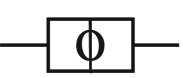
Figure 5: A phase shifter of phase $\phi$.

A beam splitter is described by:

$$U=\left(\begin{array}[]{cc}\cos\theta&-e^{i\phi}\sin\theta\\ e^{-i\phi}\sin\theta&\cos\theta\\ \end{array}\right)$$ (27)

where the input modes are related to the output modes via

$$a^{\dagger}_{l}|{0}\rangle\rightarrow\sum_{m}U_{ml}a^{\dagger}_{m}|{0}\rangle$$

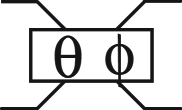
Figure 6: A beam splitter of angle $\theta$ and phase $\phi$.

The basic resources that are necessary for linear optical quantum computing are single photon sources and detectors that can distinguish between 0,1 and 2 photons.

2.2 Qubits in LOQC

In LOQC we encode qubits with dual rail logic. That is, logic that is encoded using the physical location of a photon. Logical 0 is given by $|{0}\rangle_{q}=|{01}\rangle_{ab}$ and logical 1 by $|{1}\rangle_{q}=|{10}\rangle_{ab}$, where mode $a$ is one spatial mode and mode $b$ another.

We could just as easily use photon polarisation: $|{0}\rangle_{q}=|{H}\rangle$, $|{1}\rangle_{q}=|{V}\rangle$. We can change the representation of the qubit from polarisation to spatial mode using a polarising rotator and a polarising beam splitter as can be seen below in fig. 7.

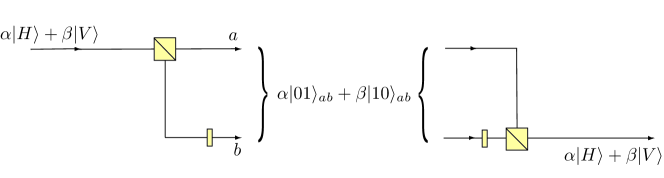
Figure 7: Transforming from dual rail to polarisation encoding.

The polarisation encoding of qubits is useful to understand some of the experimental implementation of LOQC but for this and subsequent lectures we will be using dual rail encoding for qubits.

2.3 Qubit Operations

For a physical system to be a viable candidate for quantum computation, we need a universal set of gates, as stated in point 3 of DiVincenzo’s five criteria [1], seen in section 1.2. Such a universal set is comprised of arbitrary single qubit gates and the CNOT operation [13].

We will show that single qubit operations are easily performed using linear elements and almost always error free. However, as we saw last lecture, it is quite difficult to make photons interact. We will show that with the use of single photon ancillas and photo-detection we can make a two qubit gate (a control phase gate). The non-linearity will still be there, in the form of measurement. Unfortunately this two qubit gate will not be unitary but using quantum teleportation and quantum error correction we will be able to approximate a unitary operation using only a polynomial amount of resources.

2.4 Single qubit gates

All single qubit gates can be implemented with just beam splitters and phase shifters. To see this, note that any single qubit unitary, $U$, can be decomposed into rotations about the $Z$ and $Y$ axis in the Bloch sphere as follows [5]:

$$U=e^{i\alpha}R_{z}(\beta)R_{y}(\gamma)R_{z}(\delta)$$

where $R_{z}(\theta)=e^{-i\frac{\theta}{2}\sigma_{z}}$ and $R_{y}(\phi)=e^{-i\frac{\phi}{2}\sigma_{y}}$. Exercise: show that $R_{x}(\vartheta)=R_{z}(\frac{\pi}{2})R_{y}(-\vartheta)R_{z}(-\frac{\pi}{2})$.

If we can show how to make arbitrary rotations about the $Z$ and $Y$ axis we can perform any arbitrary single qubit operation.

Rotations about the $Z$ axis can simply be performed using a phase shifter on the top mode of a qubit:

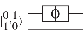
Figure 8: Performs a rotation of $\phi$ about the $Z$ axis: $R_{Z}(\phi)$.

Consider the effect of the above circuit on the qubit $\alpha|{0}\rangle_{q}+\beta|{1}\rangle_{q}$:

$$\alpha|{0}\rangle_{q}+\beta|{1}\rangle_{q} = \alpha|{01}\rangle+\beta|{10}\rangle$$

$$\rightarrow \alpha|{01}\rangle+\beta e^{i\phi}|{10}\rangle$$

$$= e^{i\phi/2}(e^{-i\phi/2}\alpha|{0}\rangle_{q}+e^{i\phi/2}\beta|{1}\rangle_{q})$$

$$= e^{i\phi/2}e^{-i\phi Z_{q}/2}(\alpha|{0}\rangle_{q}+\beta|{1}\rangle_{q})$$

$$= e^{i\phi/2}R_{Z}(\phi)(\alpha|{0}\rangle_{q}+\beta|{1}\rangle_{q})$$

And we see that, up to an irrelevant global phase, a $R_{Z}(\phi)$ has been performed.

Rotations of $-2\theta$ about the $Y$ axis require a beam splitter of angle $\theta$ and angle $\phi=0$:

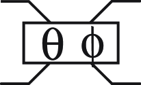
Figure 9: Performs a rotation of $-2\theta$ about the $Y$ axis: $R_{Y}(-2\theta)$.

We can see this by first remembering the effect of a beam splitter on a photon in modes 1 and 2:

$$\hat{a}_{1}^{\dagger} \rightarrow \bigl{(}\cos(\theta)\hat{a}_{1}^{\dagger}+\sin(\theta)\hat{a}_{2}^{\dagger}\bigr{)}$$

$$\hat{a}_{2}^{\dagger} \rightarrow \bigl{(}-\sin(\theta)\hat{a}_{1}^{\dagger}+\cos(\theta)\hat{a}_{2}^{\dagger}\bigr{)}$$

We can consider the effect of the above circuit on the qubit $\alpha|{0}\rangle_{q}+\beta|{1}\rangle_{q}$:

$$\alpha|{0}\rangle_{q}+\beta|{1}\rangle_{q} = \alpha|{01}\rangle+\beta|{10}\rangle$$

$$\rightarrow \alpha\bigl{(}\cos(\theta)|{01}\rangle-\sin(\theta)|{10}\rangle\bigr{)}+\beta\bigl{(}\cos(\theta)|{10}\rangle+\sin(\theta)|{01}\rangle\bigr{)}$$

$$= \cos(\theta)\bigl{(}\alpha|{01}\rangle+\beta|{10}\rangle\bigr{)}-\sin(\theta)\bigl{(}\alpha|{10}\rangle-\beta|{01}\rangle\bigr{)}$$

$$= e^{i\theta Y_{q}}\bigl{(}\alpha|{0}\rangle_{q}+\beta|{1}\rangle_{q}\bigr{)}$$

$$= R_{Y}(-2\theta)\bigl{(}\alpha|{0}\rangle_{q}+\beta|{1}\rangle_{q}\bigr{)}$$

2.5 Two qubit gates

Now we have to address the question of how to make a CNOT gate with just single photon ancillas and photo-detection. We will actually be looking at how we can perform a CSign, the relation between the two is apparent from the fact that $HZH=X$. The CSign gate has the action $|{x}\rangle_{L}|{y}\rangle_{L}\to e^{i\pi x\cdot y}|{x}\rangle_{L}|{y}\rangle_{L}$, $x,y\in\{0,1\}$.

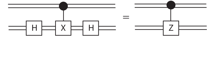
Figure 10: The equivalence between a CNOT and a CSign.

We will first show how to perform a probabilistic CSign gate on photonic qubits. From here we will show how the CSign probability of success can be boosted arbitrarily close to 1 using teleportation. In the next section we will see how this could be simplified even further by using quantum error correction.

To perform a CSign gate we need a basic transformation: $\alpha|{0}\rangle+\beta|{1}\rangle+\gamma|{2}\rangle\to\alpha|{0}\rangle+\beta|{1}\rangle-\gamma|{2}\rangle$. This is called a non-linear sign shift $NS_{-1}$. Exercise: why is the transformation non-linear?

2.5.1 Nonlinear sign shift gate

As the above transformation is non-linear we cannot use linear optics alone. We find that with the use of ancilla modes and photo-detection we can indeed perform this transformation using two extra modes, one with a single photon and the other in vacuum as shown in the circuit below. The input state looks like $\bigl{(}\alpha|{0}\rangle_{1}+\beta|{1}\rangle_{1}+\gamma|{2}\rangle_{1}\bigr{)}\otimes|{1}\rangle_{2}\otimes|{0}\rangle_{3}$.

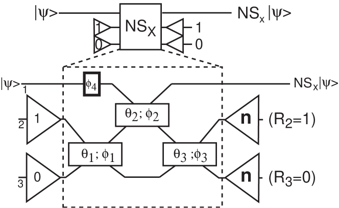
Figure 11: The $NS_{-1}$ gate.

Where $\theta_{1}=22.5^{\circ},\phi_{1}=0^{\circ}$, $\theta_{2}=65.5302^{\circ},\phi_{2}=0^{\circ}$, $\theta_{3}=-22.5^{\circ},\phi_{3}=0^{\circ}$ and $\phi_{4}=\pi^{\circ}$.

The action of this circuit is to apply the following unitary matrix on the input modes:

$$U\left(\begin{array}[]{ccc}\hat{a}_{1}^{\dagger}\\ \hat{a}_{2}^{\dagger}\\ \hat{a}_{3}^{\dagger}\end{array}\right)=\left(\begin{array}[]{ccc}1-\sqrt{2}&\frac{1}{\sqrt{\sqrt{2}}}&\sqrt{\frac{3}{\sqrt{2}}-2}\\ \frac{1}{\sqrt{\sqrt{2}}}&\frac{1}{2}&\frac{1}{2}-\frac{1}{\sqrt{2}}\\ \sqrt{\frac{3}{\sqrt{2}}-2}&\frac{1}{2}-\frac{1}{\sqrt{2}}&\sqrt{2}-\frac{1}{2}\\ \end{array}\right)\left(\begin{array}[]{ccc}\hat{a}_{1}^{\dagger}\\ \hat{a}_{2}^{\dagger}\\ \hat{a}_{3}^{\dagger}\end{array}\right)$$

Does this look familiar? Remember lecture 1.

When we measure a single photon in mode 2 and vacuum in mode 3 we have the state $\alpha|{0}\rangle_{1}+\beta|{1}\rangle_{1}-\gamma|{2}\rangle_{1}$ output in mode 1. The probability of measuring a single photon in mode 2 and vacuum in mode 3 is $\frac{1}{4}$.

Exercise: show that this circuit indeed performs the transformation $\alpha|{0}\rangle+\beta|{1}\rangle+\gamma|{2}\rangle\to\alpha|{0}\rangle+\beta|{1}\rangle-\gamma|{2}\rangle$ when mode 2 and 3 are measured in $|{10}\rangle$ and that this succeeds with probability $1/4$.

2.5.2 Controlled Sign gate

With the use of two $NS_{-1}$ gates we can make a CSign gate, as seen in the fig. below.

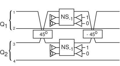
Figure 12: A probabilistic CSign gate. The probability of success $\frac{1}{16}$.

Lets work through a general example, say we start with the input state $Q_{1}=\alpha|{0}\rangle_{q}+\beta|{1}\rangle_{q}=\alpha|{01}\rangle+\beta|{10}\rangle$ in modes 1 and 2 and $Q_{2}=\gamma|{0}\rangle_{q}+\delta|{1}\rangle_{q}=\gamma|{01}\rangle+\delta|{10}\rangle$ in modes 3 and 4.

After the first beam splitter we have

$$\alpha\gamma|{0101}\rangle+\alpha\delta|{0110}\rangle+\beta\gamma|{1001}\rangle+\beta\delta|{1010}\rangle$$

$$\to \alpha\gamma|{0101}\rangle-\frac{\alpha\delta}{\sqrt{2}}|{1100}\rangle+\frac{\alpha\delta}{\sqrt{2}}|{0110}\rangle+\frac{\beta\gamma}{\sqrt{2}}|{1001}\rangle$$

$$\,\,+\frac{\beta\gamma}{\sqrt{2}}|{0011}\rangle-\frac{\beta\delta}{\sqrt{2}}|{2000}\rangle+\frac{\beta\delta}{\sqrt{2}}|{0020}\rangle$$

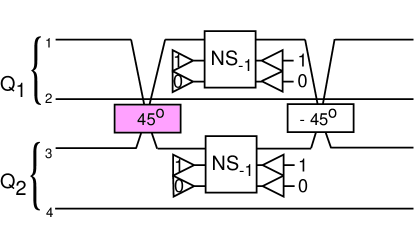
Figure 13: Step 1 of a probabilistic CSign gate.

After the two $NS_{-1}$ gates we have

$$\to \alpha\gamma|{0101}\rangle-\frac{\alpha\delta}{\sqrt{2}}|{1100}\rangle+\frac{\alpha\delta}{\sqrt{2}}|{0110}\rangle+\frac{\beta\gamma}{\sqrt{2}}|{1001}\rangle$$

$$\,\,+\frac{\beta\gamma}{\sqrt{2}}|{0011}\rangle+\frac{\beta\delta}{\sqrt{2}}|{2000}\rangle-\frac{\beta\delta}{\sqrt{2}}|{0020}\rangle$$

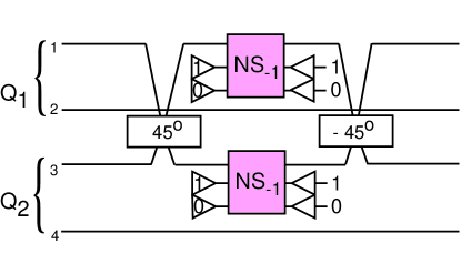
Figure 14: Step 2 of a probabilistic CSign gate.

After the final beam splitter we have

$$\to \alpha\gamma|{0101}\rangle+\alpha\delta|{0110}\rangle+\beta\gamma|{1001}\rangle-\beta\delta|{1010}\rangle$$

$$= \alpha\gamma|{00}\rangle_{q}+\alpha\delta|{01}\rangle_{q}+\beta\gamma|{10}\rangle_{q}-\beta\delta|{11}\rangle_{q}$$

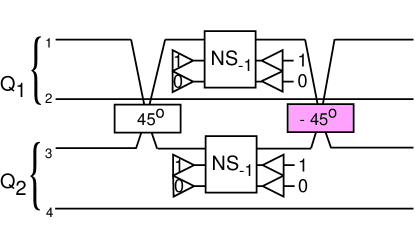
Figure 15: Step 3 of a probabilistic CSign gate.

This gate works with a probability of $\frac{1}{16}$. That is, there is a probability of $\frac{1}{16}$ that we will measure the ancilla state $|{10}\rangle$ in both $NS_{-1}$ gates. It is important to notice that when the result of the measurement of the ancilla state is other than $|{10}\rangle$, the gate fails but we know that this failure has occurred.

It is also interesting that during the gate, between the $\pm 45^{\circ}$ beam splitters, the photons are not in the dual rail logic encoding but recombine at the last beam splitter to get back into the right encoding. Thus we go out of the qubits Hilbert space to make this gate and go back at its output.

The state

$$\frac{1}{2}\Bigl{(}|{0101}\rangle+|{0110}\rangle+|{1001}\rangle-|{1010}\rangle\Bigr{)}$$ (29)

is the first building block to performing a CSign on photonic qubits with probability arbitrarily close to 1.

2.5.3 Teleporting qubits through a gate

What we have shown so far is how to perform a probabilistic CSign gate on photonic qubits. This is not enough to allow scalable quantum computation. The probabilistic CSign gate will be used as an entangled state production stage.

To perform a two qubit gate we could teleport [14] the qubits through the gate as first shown by Gottesman and Chuang [15].

Say we have two arbitrary qubits $|{\psi_{1}}\rangle_{q}$ and $|{\psi_{2}}\rangle_{q}$ that we want to perform a CSign on. We could teleport both these qubits and then apply a CSign on them, as seen in the fig. below:

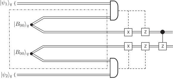
Figure 16: An application a CSign between qubits $|{\psi_{1}}\rangle_{q}$ and $|{\psi_{2}}\rangle_{q}$. The dashed-dotted box is the state preparation area. In this case just the Bell states $|{B_{00}}\rangle$ need to be prepared.

Exercise: given that $|{B_{00}}\rangle_{q}=\frac{1}{\sqrt{2}}\bigl{(}|{00}\rangle+|{11}\rangle\bigr{)}_{q}$, $|{\psi_{1}}\rangle_{q}=c_{0}|{0}\rangle_{q}+c_{1}|{1}\rangle_{q}$, $|{\psi_{2}}\rangle_{q}=d_{0}|{0}\rangle_{q}+d_{1}|{1}\rangle_{q}$ (all logical qubits, $|c_{0}|^{2}+|c_{1}|^{2}=|d_{0}|^{2}+|d_{1}|^{2}=1$), and that we measure in the logical basis, show that this circuit gives a CSign between $|{\psi_{1}}\rangle_{q}$ and $|{\psi_{2}}\rangle_{q}$.

Since CSign applied twice gives the identity, we can add two CSign’s to fig. 16 as seen in fig. 17.

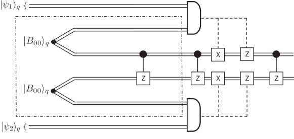
Figure 17: An application a CSign between qubits $|{\psi_{1}}\rangle_{q}$ and $|{\psi_{2}}\rangle_{q}$.

We now have a CSign inside the dashed-dotted box, the state preparation area. Now we want to look at the effect of conjugating the “corrections” with the CSign’s. To do this we will need the identity:

$$\text{CSign}\Bigl{(}\sigma_{x}\otimes{\mathchoice{\rm 1\mskip-4.0mul}{\rm 1\mskip-4.0mul}{\rm 1\mskip-4.5mul}{\rm 1\mskip-5.0mul}}\Bigr{)}\text{CSign} = \sigma_{x}\otimes\sigma_{z}$$

$$\left(\begin{array}[]{cccc}1&0&0&0\\ 0&1&0&0\\ 0&0&1&0\\ 0&0&0&-1\\ \end{array}\right)\left(\begin{array}[]{cccc}0&0&1&0\\ 0&0&0&1\\ 1&0&0&0\\ 0&1&0&0\\ \end{array}\right)\left(\begin{array}[]{cccc}1&0&0&0\\ 0&1&0&0\\ 0&0&1&0\\ 0&0&0&-1\\ \end{array}\right) = \left(\begin{array}[]{cccc}0&0&1&0\\ 0&0&0&-1\\ 1&0&0&0\\ 0&-1&0&0\\ \end{array}\right)$$

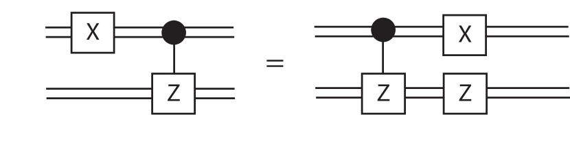
Figure 18: Shows the identity $\text{CSign}\Bigl{(}\sigma_{x}\otimes{\mathchoice{\rm 1\mskip-4.0mul}{\rm 1\mskip-4.0mul}{\rm 1\mskip-4.5mul}{\rm 1\mskip-5.0mul}}\Bigr{)}\text{CSign}=\sigma_{x}\otimes\sigma_{z}$.

and the identities

$$\text{CSign}\Bigl{(}{\mathchoice{\rm 1\mskip-4.0mul}{\rm 1\mskip-4.0mul}{\rm 1\mskip-4.5mul}{\rm 1\mskip-5.0mul}}\otimes\sigma_{x}\Bigr{)}\text{CSign} = \sigma_{z}\otimes\sigma_{x}$$

$$\text{CSign}\Bigl{(}\sigma_{z}\otimes{\mathchoice{\rm 1\mskip-4.0mul}{\rm 1\mskip-4.0mul}{\rm 1\mskip-4.5mul}{\rm 1\mskip-5.0mul}}\Bigr{)}\text{CSign} = \sigma_{z}\otimes{\mathchoice{\rm 1\mskip-4.0mul}{\rm 1\mskip-4.0mul}{\rm 1\mskip-4.5mul}{\rm 1\mskip-5.0mul}}$$

$$\text{CSign}\Bigl{(}{\mathchoice{\rm 1\mskip-4.0mul}{\rm 1\mskip-4.0mul}{\rm 1\mskip-4.5mul}{\rm 1\mskip-5.0mul}}\otimes\sigma_{z}\Bigr{)}\text{CSign} = {\mathchoice{\rm 1\mskip-4.0mul}{\rm 1\mskip-4.0mul}{\rm 1\mskip-4.5mul}{\rm 1\mskip-5.0mul}}\otimes\sigma_{z}$$

Applying these identities gives the following circuit:

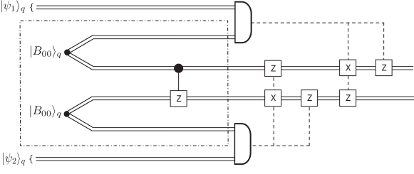
Figure 19: An application a CSign between qubits $|{\psi_{1}}\rangle_{q}$ and $|{\psi_{2}}\rangle_{q}$.

The problem of performing a CSign has now been turned into a state preparation problem. We can apply the CSign gate (fig. 12) probabilistically offline. Once we know we have a successful CSign state (eq. (29)), we can proceed and teleport the information qubits, as in fig. 19. This way we do not corrupt the quantum information.

2.5.4 Teleporting with the C-Sign entangled states

If a gate fails with probability $f$ and we perform error correction, after we do $k$ of these gates we will have a success probability of $f^{k}$. With teleportation, constructing two qubit gates reduces to a state preparation problem. The critical element is that we know when the state preparation fails and thus we can ensure that it does not corrupt the quantum information. To succeed we need to attempt the state preparation $\frac{k}{f}$ times to implement $k$ gates.

The next step is to show how we perform teleportation with linear optics?

2.5.5 Basic Teleportation with linear optics

It is known [12] that we cannot distinguish between the four Bell states with linear optics alone. With a single beam splitter the best that we can do is distinguish between the Bell states, and thus do teleportation, with a success probability of $\frac{1}{2}$. We will show how this is done and then generalise the teleportation so that the probability of success is as near to one as desired. Although we cannot achieve a probability of one as this would require perfect Bell state distinguishability, we can use quantum error correction and limit the left over error so that it is smaller than what is required from the accuracy threshold theorem.

Consider teleporting the state $\alpha|{01}\rangle+\beta|{10}\rangle$. We need only look at teleporting the first mode of this state:

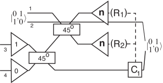
Figure 20: Telelportation with linear optics.

First the entangled resource state $\frac{1}{\sqrt{2}}\bigl{(}|{01}\rangle_{34}+|{10}\rangle_{34}\bigr{)}$ is made, shown below. At this point the state is

$$\Bigl{(} \alpha|{01}\rangle_{12}+\beta|{10}\rangle_{12}\Bigr{)}\frac{1}{\sqrt{2}}\Bigl{(}|{01}\rangle_{34}+|{10}\rangle_{34}\Bigr{)}$$

$$= \frac{1}{\sqrt{2}}\Bigl{(}\alpha|{0101}\rangle_{1234}+\alpha|{0110}\rangle_{1234}+\beta|{1001}\rangle_{1234}+\beta|{1010}\rangle_{1234}\Bigr{)}$$

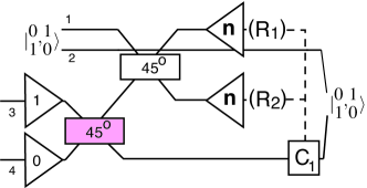
Figure 21: Telelportation with linear optics: making the entanglement resource state.

After the second beam splitter we have:

$$\to\frac{1}{2}\Bigl{(}\sqrt{2}\alpha|{0101}\rangle-\alpha|{1100}\rangle+\alpha|{0110}\rangle+\beta|{1001}\rangle+\beta|{0011}\rangle-\beta|{2000}\rangle+\beta|{0020}\rangle\Bigr{)}$$

Remembering that the second mode was unchanged here.

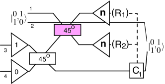
Figure 22: Telelportation with linear optics: performing a partial Bell measurement.

If the detectors measure a total of 1 photon ($R_{1}+R_{2}=1$), we can recover the original information in modes 4 and 2:

$$R_{1}=0,R_{2}=1 : \quad\frac{1}{2}\bigl{(}\alpha|{01}\rangle+\beta|{10}\rangle\bigr{)}$$

$$R_{1}=1,R_{2}=0 : \quad\frac{1}{2}\bigl{(}-\alpha|{01}\rangle+\beta|{10}\rangle\bigr{)}$$

Figure 23: Telelportation with linear optics: photo-detection.

In the case that we measure $R_{1}=1,R_{2}=0$ we need to perform a phase shift correction gate $C_{1}$ and we have seen how to do that in the previous section. The probability of successful teleportation is $\frac{1}{4}+\frac{1}{4}=\frac{1}{2}$. If the detectors measure 0 or 2 photons the teleportation fails by collapsing the state in the mode $|{0}\rangle$ or $|{1}\rangle$ and this is equivalent to projecting the qubit in the $Z$ basis, as will be explained in the next section. This occurs with a probability of $\frac{1}{2}$.

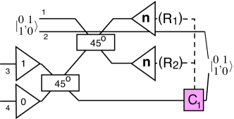
Figure 24: Telelportation with linear optics: applying a correction.

2.5.6 The teleported C-Sign

Now we can piece together what we have worked out so far to make a CSign gate. First we have the CSign entangled state production step:

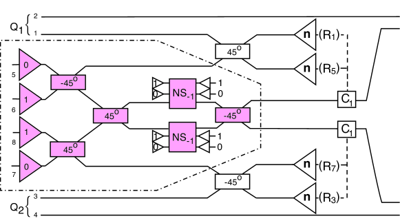
Figure 25: CSign state production

Followed by the teleportation:

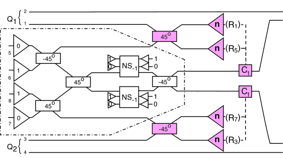
Figure 26: Teleportation.

The success probability for the state production stage (fig. 25) is $\frac{1}{16}$, however this is done offline. This state preparation fails (on average 16 times) when the measurement of the ancilla give the wrong result and then we just need to repeat the state preparation. This failure does not corrupt the quantum information as the qubtis have not yet interacted with these photons. When the measurement of the ancilla give the right values, we know that the state is the correct one for teleportation.

The success probability for this CSign gate is $\frac{1}{2}$. Exercise: given that the dashed-dotted box in fig. 25 makes a state of the form $\frac{1}{2}\bigl{(}|{1010}\rangle+|{1001}\rangle-|{0110}\rangle+|{0101}\rangle\bigr{)}_{5687}$, show that this circuit executes a C-sign between $Q_{1}$ and $Q_{2}$. Exercise: what error occurs on the information qubits if the detectors $R_{1},R_{3},R_{5}$ and $R_{7}$ do not measure the correct sequence?

2.5.7 Increasing the probability of success

The task that remains now is to improve the probability of success of the teleportation. If we increase the complexity of the state produced in the dashed-dotted box of fig. 25, we can increase the teleportation success probability asymptotically close to one. We can generalise eq. (29) by increasing the number of modes:

$$|{t_{n}}\rangle=\frac{1}{\sqrt{n+1}}\sum_{j=0}^{n}|{1}\rangle^{j}|{0}\rangle^{n-j}|{0}\rangle|{1}\rangle^{n-j}$$

where the exponent $k$ means that this state is repeated $k$ times, i.e. $|{1}\rangle^{2}\rightarrow|{1}\rangle|{1}\rangle$.

Or in the logical basis

$$|{t_{n}}\rangle_{q}=\frac{1}{\sqrt{n+1}}\sum_{j=0}^{n}|{0}\rangle_{q}^{j}|{1}\rangle_{q}^{n-j}$$

When we use this preparation state for teleportation the success probability scales as $\frac{n}{n+1}=1-\frac{1}{n+1}$.

2.5.8 Generalised beam splitter

When we use the larger entangled state $|{t_{n}}\rangle$ we need to use a generalised beam splitter: the $n+1$ point Fourier transform.

We define the $n+1$ point Fourier transform with $\hat{F}_{n+1}$. The matrix elements are given by

$$u\bigl{(}\hat{F}_{n+1}\bigr{)}_{kl}=\frac{e^{i\frac{2\pi kl}{n+1}}}{\sqrt{n+1}}$$

Exercise: show that for $n=1$ we get back our anti-symmetric 50-50 beam splitter transformation.

As in fig. 23, we measure all the outputs of the $n+1$ point Fourier transform. If we detect $k$ photons and $0<k<n+1$, then we know the qubit has been teleported to mode $n+k$. If we measure either 0 or $n+1$ photons the teleportation has failed.

For example, consider the case when $n=2$:

$$|{t_{2}}\rangle=\frac{1}{\sqrt{3}}\Bigl{(}|{0011}\rangle+|{1001}\rangle+|{1100}\rangle\Bigr{)}$$

and

$$u(F_{3})=\left(\begin{array}[]{ccc}1&1&1\\ 1&e^{\frac{2\pi i}{3}}&e^{-\frac{2\pi i}{3}}\\ 1&e^{-\frac{2\pi i}{3}}&e^{\frac{2\pi i}{3}}\\ \end{array}\right)$$

Exercise: Find the linear circuit that implement this unitary transformation.

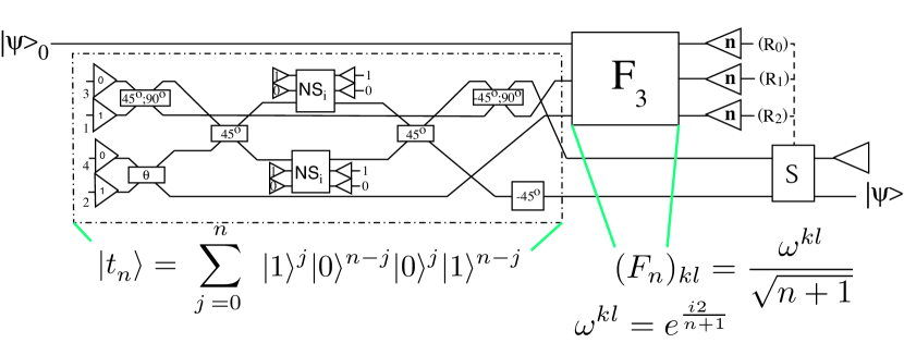
Figure 27: Teleportation with $|{t_{2}}\rangle$. The dashed-dotted box produces $|{t_{2}}\rangle$. The probability of success of this teleportation is 2/3.

When $F_{3}$ is applied to the incident modes 0, 1 and 2, the modes are transformed as follows:

$$\hat{a}_{0}^{\dagger} \to \frac{1}{\sqrt{3}}\bigl{(}\hat{a}_{0}^{\dagger}+\hat{a}_{1}^{\dagger}+\hat{a}_{2}^{\dagger}\bigr{)}$$

$$\hat{a}_{1}^{\dagger} \to \frac{1}{\sqrt{3}}\bigl{(}\hat{a}_{0}^{\dagger}+e^{\frac{2\pi i}{3}}\hat{a}_{1}^{\dagger}+e^{-\frac{2\pi i}{3}}\hat{a}_{2}^{\dagger}\bigr{)}$$

$$\hat{a}_{2}^{\dagger} \to \frac{1}{\sqrt{3}}\bigl{(}\hat{a}_{0}^{\dagger}+e^{-\frac{2\pi i}{3}}\hat{a}_{1}^{\dagger}+e^{\frac{2\pi i}{3}}\hat{a}_{2}^{\dagger}\bigr{)}$$

Now say we want to teleport the state $\alpha|{01}\rangle+\beta|{10}\rangle$ (where the second mode of this state propagates unchanged) with the entangled resource state $|{t_{2}}\rangle$.

Once we apply the 3 point Fourier transform to the states $\alpha|{01}\rangle+\beta|{10}\rangle$ and $|{t_{2}}\rangle$, we have 19 measurement outcomes: $R_{0},R_{1},R_{2}=$ 000, 001, 010, 100, 011, 101, 110, 002, 020, 200, 012, 021, 201, 102, 120, 210, 300, 030 and 003. We are only interested in measuring total photon numbers between 0 and $n+1=3$, that is, only 1 or 2 photons in total.

The measurement outcomes we are interested in are given in the table below, along with the mode the information is output in and the probability of that measurement. The following identities will be useful when working through this example: $e^{i\frac{2}{3}\pi}+e^{-i\frac{2}{3}\pi}=-1$, $e^{i\frac{4}{3}\pi}+e^{-i\frac{4}{3}\pi}=-1$, $e^{i\frac{2}{3}\pi}+1=e^{i\frac{\pi}{3}}$ and $e^{-i\frac{2}{3}\pi}+1=e^{-i\frac{\pi}{3}}$

The total probability for successful teleportation is $3\bigl{(}\frac{1}{9}\bigr{)}+3\bigl{(}\frac{2}{27}\bigr{)}+3\bigl{(}\frac{1}{27}\bigr{)}=\frac{2}{3}$. This corresponds to $\frac{n}{n+1}$ with n=2. As in the case of the previous subsubsection, when the teleportation fails we know it and then the state is projected in the $Z$ basis.

Measurement	Output	Mode	Probability
$|{100}\rangle$	$\frac{1}{3}\bigl{(}\alpha|{0}\rangle+\beta|{1}\rangle\bigr{)}$	3	$\frac{1}{9}$
$|{010}\rangle$	$\frac{1}{3}\bigl{(}e^{\frac{2\pi i}{3}}\alpha|{0}\rangle+\beta|{1}\rangle\bigr{)}$	3	$\frac{1}{9}$
$|{001}\rangle$	$\frac{1}{3}\bigl{(}e^{-\frac{2\pi i}{3}}\alpha|{0}\rangle+\beta|{1}\rangle\bigr{)}$	3	$\frac{1}{9}$
$|{200}\rangle$	$\frac{\sqrt{2}}{3\sqrt{3}}\bigl{(}\alpha|{0}\rangle+\beta|{1}\rangle\bigr{)}$	4	$\frac{2}{27}$
$|{020}\rangle$	$\frac{\sqrt{2}}{3\sqrt{3}}\bigl{(}\alpha|{0}\rangle+e^{\frac{2\pi i}{3}}\beta|{1}\rangle\bigr{)}$	4	$\frac{2}{27}$
$|{002}\rangle$	$\frac{\sqrt{2}}{3\sqrt{3}}\bigl{(}\alpha|{0}\rangle+e^{-\frac{2\pi i}{3}}\beta|{1}\rangle\bigr{)}$	4	$\frac{2}{27}$
$|{110}\rangle$	$\frac{1}{3\sqrt{3}}\bigl{(}-\alpha|{0}\rangle+e^{\frac{i\pi}{3}}\beta|{1}\rangle\bigr{)}$	4	$\frac{1}{27}$
$|{101}\rangle$	$\frac{1}{3\sqrt{3}}\bigl{(}-\alpha|{0}\rangle+e^{-\frac{i\pi}{3}}\beta|{1}\rangle\bigr{)}$	4	$\frac{1}{27}$
$|{011}\rangle$	$\frac{1}{3\sqrt{3}}\bigl{(}-\alpha|{0}\rangle-\beta|{1}\rangle\bigr{)}$	4	$\frac{1}{27}$

Table 2: The telelported states when using $|{t_{2}}\rangle$ as an entanglement resource.

2.5.9 Bounds on success probabilities

We have shown in this lecture that we can perform the $NS_{-1}$ gate operation $\alpha|{0}\rangle+\beta|{1}\rangle+\gamma|{2}\rangle\to\alpha|{0}\rangle+\beta|{1}\rangle-\gamma|{2}\rangle$ with a success probability of $\frac{1}{4}$ (fig. 11). We have also shown that using two of these $NS_{-1}$ gates we can perform a CSign with success probability $\frac{1}{16}$ (fig. 12). However, it is not known whether these probabilities are optimal.

To date, the best $NS_{-1}$ gate success probability is as above and the best CSign gate succeeds with a probability of $\frac{2}{27}$ [16]. The $\frac{2}{27}$ CSign gate is shown in fig. 28.

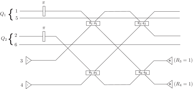
Figure 28: A CSign gate with success probability $\frac{2}{27}$. Here $\theta_{1}=54.74^{o},\phi_{1}=0$, $\theta_{2}=-54.74^{o},\phi_{2}=0$, $\theta_{3}=54.74^{o},\phi_{3}=0$ and $\theta_{4}=17.63^{o},\phi_{4}=0$.

In this circuit the two qubits $Q_{1}:\alpha|{01}\rangle_{15}+\beta|{10}\rangle_{15}$ and $Q_{2}:\gamma|{01}\rangle_{26}+\delta|{10}\rangle_{26}$ are to have a CSign applied, where modes 5 and 6 are left unchanged. Exercise: check that this circuit implements a CSign on measuring single photons in modes 3 and 4.

Knill has shown that the CSign gate has an upper bound of $\frac{3}{4}$ when using two ancilla modes, each with a maximum of 1 photon per mode [17]. Knill has also shown that the upper bound for any $NS_{-1}$ gate with one ancilla mode is $\frac{1}{2}$ [17]. Scheel et. al. conjecture that the upper bound for the $NS_{-1}$ gate is $\frac{1}{4}$, regardless of the dimensionality of the ancilla space [18].

3 LOQC and Quantum Error Correction

3.1 Improving LOQC: beyond state preparation

In the last section we showed that scalable quantum computing was possible with linear optical elements, single photon sources and photo-detection. The problem of making a two qubit gate with probability of success arbitrarily close to one was transferred to a state preparation problem. By using generalised entangled states of the form $|{t_{n}}\rangle$, the probability of success scaled as $\frac{n}{n+1}$. However, states of the form $|{t_{n}}\rangle$ are complicated to make. To date the best schemes need resources that are exponential in $n$ [19, 20]. Instead, we may ask ourselves if we can incorporate quantum error correction [21] into the LOQC proposal. Is it possible to correct for the incorrect measurements in the basic linear optical teleportation (fig. 20)? Can we use quantum error correction along with smaller $|{t_{n}}\rangle$ states to increase the probability of successful gates giving scalable quantum computing?

To answer this we first need to know what errors are inflicted on the quantum information when an incorrect measurement is made in the teleportation in fig. 20.

In the previous section we went through this basic teleportation with linear optics and showed that if we want to teleport the state $\alpha|{01}\rangle+\beta|{10}\rangle$ using the entanglement resource state $\frac{1}{\sqrt{2}}\bigl{(}|{01}\rangle+|{10}\rangle\bigr{)}$, we need to measure 1 and only 1 photon at the photo-detection stage (fig. 23). The probability of success was $\frac{1}{2}$. But what happens when we measure 0 or 2 photons?

Recalling from the last section, our input state is transformed to

$$\to\frac{1}{2}\Bigl{(}\sqrt{2}\alpha|{0101}\rangle-\alpha|{1100}\rangle+\alpha|{0110}\rangle+\beta|{1001}\rangle+\beta|{0011}\rangle-\beta|{2000}\rangle+\beta|{0020}\rangle\Bigr{)}$$

just before the measurement in fig. 23 (remembering the 2nd mode is untouched). If the detectors measure a total of 1 photon ($R_{1}+R_{2}=1$) we can recover the original information:

$$R_{1}=0,R_{2}=1 : \quad\frac{1}{2}\bigl{(}\alpha|{01}\rangle+\beta|{10}\rangle\bigr{)}$$

$$R_{0}=1,R_{1}=1 : \quad\frac{1}{2}\bigl{(}-\alpha_{0}|{01}\rangle+\alpha_{1}|{10}\rangle\bigr{)}$$

If the detectors measure a total of 0 or 2 photons ($R_{1}+R_{2}=0\,\,\text{mod}\,\,2$) we have:

$$R_{1}=0,R_{2}=0 : \quad\frac{1}{\sqrt{2}}\alpha_{0}|{11}\rangle$$

$$R_{0}=2,R_{1}=0 : \quad-\frac{1}{\sqrt{2}}\alpha_{1}|{00}\rangle$$

$$R_{1}=0,R_{2}=2 : \quad\frac{1}{\sqrt{2}}\alpha_{1}|{00}\rangle$$

Note that when we measure 0 or 2 photons we have measured our qubit, collapsing our “quantum” information. This means we are free to add a single photon, or vacuum mode. When we measure 0 photons, we obtain the state $|{01}\rangle=|{0}\rangle_{q}$ and when we measure 2 photons, we obtain $|{10}\rangle=|{1}\rangle_{q}$. When we measure 0 or 2 photons we effectively measure our information qubit in the $Z$-basis. Exercise: check that the probability of measuring 0, 1 or 2 photons in total adds to 1.

Knowing this we should be able to use quantum error correction to somehow encoded our quantum data and then correct when the teleportation fails, i.e. when the measurement give either 0 or 2 photons in fig. 23. This means we need to find quantum error correcting codes that deal with an error model corresponding with projection in the $Z$ basis, where we know which qubit was projected. From this point on we’ll be dealing with Z-measurement errors that are appearing when we try to make a two bit gate on the qubits. We will assume that the one bit gates (implemented by linear optics) are error free. But first we need to know what a quantum error correcting code is.

3.2 Quantum Error Correcting Codes

3.2.1 What are they?

We can encode our quantum information with code words to protect against errors. Classically, when the error model is given by independent bit flips $(X)$, this can be done via the repetition code: $0\to 000$ and $1\to 111$.

When we generalise the classical theory to the quantum one, we also have to worry about phase errors ($Z$ operators and the combination of bit flip and phase errors: $Y$ operators). A necessary and sufficient condition for a code with basis code words $\{|{\psi}\rangle\}$ to correct for errors $\{E\}$ is

$$\langle{\psi_{i}}|E_{a}^{\dagger}E_{b}|{\psi_{j}}\rangle=C_{ab}\delta_{ij}$$ (32)

where $|{\psi_{i}}\rangle,|{\psi_{j}}\rangle\in\{|{\psi}\rangle\}$ and $E_{a},E_{b}\in\{E\}$.

Say we have errors of the form $E_{1}=\frac{1}{2}\bigl{(}{\mathchoice{\rm 1\mskip-4.0mul}{\rm 1\mskip-4.0mul}{\rm 1\mskip-4.5mul}{\rm 1\mskip-5.0mul}}+Z\bigr{)}$, $E_{2}=\frac{1}{2}\bigl{(}{\mathchoice{\rm 1\mskip-4.0mul}{\rm 1\mskip-4.0mul}{\rm 1\mskip-4.5mul}{\rm 1\mskip-5.0mul}}-Z\bigr{)}$. What does this do to our qubit $|{\psi}\rangle=\alpha|{0}\rangle_{q}+\beta|{1}\rangle_{q}$?

$$E_{1}|{\psi}\rangle = \alpha|{0}\rangle_{q}$$

$$E_{2}|{\psi}\rangle = \beta|{1}\rangle_{q}$$

We have measured our qubit in the $Z$-basis. How can we encode to correct for this error? We could try the following encoding:

$$|{\overline{0}}\rangle = \frac{1}{\sqrt{2}}\bigl{(}|{00}\rangle_{q}+|{11}\rangle_{q}\bigr{)}$$ (33)

$$|{\overline{1}}\rangle = \frac{1}{\sqrt{2}}\bigl{(}|{01}\rangle_{q}+|{10}\rangle_{q}\bigr{)}$$ (34)

If we measure the first mode of our encoded qubit in the $Z$-basis we have

$$\frac{1}{\sqrt{2}}\bigl{(} \alpha |{00}\rangle_{q}+\alpha|{11}\rangle_{q}+\beta|{01}\rangle_{q}+\beta|{10}\rangle_{q}\bigr{)}$$

$$= \frac{1}{\sqrt{2}}\{|{0}\rangle_{q}\bigl{(}\alpha|{0}\rangle_{q}+\beta|{1}\rangle_{q}\bigr{)}\}+\frac{1}{\sqrt{2}}|{1}\rangle_{q}\bigl{(}\alpha|{1}\rangle_{q}+\beta|{0}\rangle_{q}\bigr{)}\}$$

and we see that if we measure mode 1 to be a $|{0}\rangle_{q}$, we get our original information qubit back and if we measure mode 1 to be a $|{1}\rangle_{q}$, we can get our original information qubit back once we apply a bit flip. Now we need to check that this code satisfies condition 32 for the errors $E_{1}$ and $E_{2}$. We assume the errors are on the 1st qubit, so $E_{1}=\frac{1}{2}\bigl{(}{\mathchoice{\rm 1\mskip-4.0mul}{\rm 1\mskip-4.0mul}{\rm 1\mskip-4.5mul}{\rm 1\mskip-5.0mul}}+Z\bigr{)}\otimes{\mathchoice{\rm 1\mskip-4.0mul}{\rm 1\mskip-4.0mul}{\rm 1\mskip-4.5mul}{\rm 1\mskip-5.0mul}}$ and $E_{2}=\frac{1}{2}\bigl{(}{\mathchoice{\rm 1\mskip-4.0mul}{\rm 1\mskip-4.0mul}{\rm 1\mskip-4.5mul}{\rm 1\mskip-5.0mul}}-Z\bigr{)}\otimes{\mathchoice{\rm 1\mskip-4.0mul}{\rm 1\mskip-4.0mul}{\rm 1\mskip-4.5mul}{\rm 1\mskip-5.0mul}}$:

$\langle{\overline{0}}|E_{1}^{\dagger}{\mathchoice{\rm 1\mskip-4.0mul}{\rm 1\mskip-4.0mul}{\rm 1\mskip-4.5mul}{\rm 1\mskip-5.0mul}}|{\overline{0}}\rangle=\frac{1}{2}$	$\langle{\overline{0}}|E_{2}^{\dagger}{\mathchoice{\rm 1\mskip-4.0mul}{\rm 1\mskip-4.0mul}{\rm 1\mskip-4.5mul}{\rm 1\mskip-5.0mul}}|{\overline{0}}\rangle=\frac{1}{2}$	$\langle{\overline{0}}|E_{1}^{\dagger}E_{2}|{\overline{0}}\rangle=0$	$\langle{\overline{0}}|E_{2}^{\dagger}E_{1}|{\overline{0}}\rangle=0$
$\langle{\overline{0}}|E_{1}^{\dagger}{\mathchoice{\rm 1\mskip-4.0mul}{\rm 1\mskip-4.0mul}{\rm 1\mskip-4.5mul}{\rm 1\mskip-5.0mul}}|{\overline{1}}\rangle=0$	$\langle{\overline{0}}|E_{2}^{\dagger}{\mathchoice{\rm 1\mskip-4.0mul}{\rm 1\mskip-4.0mul}{\rm 1\mskip-4.5mul}{\rm 1\mskip-5.0mul}}|{\overline{1}}\rangle$=0	$\langle{\overline{0}}|E_{1}^{\dagger}E_{2}|{\overline{1}}\rangle=0$	$\langle{\overline{0}}|E_{2}^{\dagger}E_{1}|{\overline{1}}\rangle=0$
$\langle{\overline{1}}|E_{1}^{\dagger}{\mathchoice{\rm 1\mskip-4.0mul}{\rm 1\mskip-4.0mul}{\rm 1\mskip-4.5mul}{\rm 1\mskip-5.0mul}}|{\overline{0}}\rangle=0$	$\langle{\overline{1}}|E_{2}^{\dagger}{\mathchoice{\rm 1\mskip-4.0mul}{\rm 1\mskip-4.0mul}{\rm 1\mskip-4.5mul}{\rm 1\mskip-5.0mul}}|{\overline{0}}\rangle$=0	$\langle{\overline{1}}|E_{1}^{\dagger}E_{2}|{\overline{0}}\rangle=0$	$\langle{\overline{1}}|E_{2}^{\dagger}E_{1}|{\overline{0}}\rangle=0$
$\langle{\overline{1}}|E_{1}^{\dagger}{\mathchoice{\rm 1\mskip-4.0mul}{\rm 1\mskip-4.0mul}{\rm 1\mskip-4.5mul}{\rm 1\mskip-5.0mul}}|{\overline{1}}\rangle=\frac{1}{2}$	$\langle{\overline{1}}|E_{2}^{\dagger}{\mathchoice{\rm 1\mskip-4.0mul}{\rm 1\mskip-4.0mul}{\rm 1\mskip-4.5mul}{\rm 1\mskip-5.0mul}}|{\overline{1}}\rangle=\frac{1}{2}$	$\langle{\overline{1}}|E_{1}^{\dagger}E_{2}|{\overline{1}}\rangle=0$	$\langle{\overline{1}}|E_{2}^{\dagger}E_{1}|{\overline{1}}\rangle=0$

Table 3: Testing condition 32 for the errors $E_{1}$ and $E_{2}$.

But this doesn’t tell us how to correct for the errors $E_{1}$ and $E_{2}$, only that correction is possible.

3.2.2 $Z$-measurement Quantum Error Correcting Code (QECC)

How can we correct for the Z-measurement errors $E_{1}$ and $E_{2}$? There is a formalism called the stabilizer formalism (see [22]) that gives us a way to do this. The stabilizer is defined by a set of operators for an $n$ qubit system whose common eigenvectors define a $2^{k}$-dimensional subspace (the code). That is, the stabilizer is defined as the set of operators $\{M_{i}\}$ that leave the code word space $\{|{\overline{\psi_{j}}}\rangle\}$ invariant: $M_{i}|{\overline{\psi_{j}}}\rangle=|{\overline{\psi_{j}}}\rangle\,\,\forall i,j$. We will focus on operators formed by tensor products of Pauli operators. We have the two code words: $|{\overline{0}}\rangle=\frac{1}{\sqrt{2}}\bigl{(}|{00}\rangle_{q}+|{11}\rangle_{q}\bigr{)}$ and $|{\overline{1}}\rangle=\frac{1}{\sqrt{2}}\bigl{(}|{01}\rangle_{q}+|{10}\rangle_{q}\bigr{)}$. These are stabilized by the two operators ${\mathchoice{\rm 1\mskip-4.0mul}{\rm 1\mskip-4.0mul}{\rm 1\mskip-4.5mul}{\rm 1\mskip-5.0mul}}\otimes{\mathchoice{\rm 1\mskip-4.0mul}{\rm 1\mskip-4.0mul}{\rm 1\mskip-4.5mul}{\rm 1\mskip-5.0mul}}$ and $X\otimes X$. Exercise: check that $XX$ stabilizer the $Z$-measurement code.

For a stabilizer code we can detect all errors that are either in the stabilizer or anti-commute with any member of the stabilizer group. Say we have the QECC with code words $|{\overline{\psi}_{j}}\rangle$ and $M_{i}$ is an element of the stabilizer $S$. And say $E$ is an error such that $\{M_{i},E\}=0$, then $M_{i}E|{\overline{\psi}_{j}}\rangle=-EM_{i}|{\overline{\psi}_{j}}\rangle=-E|{\overline{\psi}_{j}}\rangle$. So $E|{\overline{\psi}_{j}}\rangle$ is an eigenstate of $M_{i}$, so measuring $M_{i}$ will tell us if $E$ has occurred. By measuring all the stabilizer generators we identify the error syndrome with this method.

If a QECC can correct for errors $E$ and $F$, then it can also correct for the error $aE+bF$. From the form of $E_{1}$ and $E_{2}$ we need only consider correcting the error $Z\otimes{\mathchoice{\rm 1\mskip-4.0mul}{\rm 1\mskip-4.0mul}{\rm 1\mskip-4.5mul}{\rm 1\mskip-5.0mul}}$. More generally, when we consider correcting for a $Z$-measurement error on either qubit of the code words (33), (34), we need to consider the errors $Z\otimes{\mathchoice{\rm 1\mskip-4.0mul}{\rm 1\mskip-4.0mul}{\rm 1\mskip-4.5mul}{\rm 1\mskip-5.0mul}}$ and ${\mathchoice{\rm 1\mskip-4.0mul}{\rm 1\mskip-4.0mul}{\rm 1\mskip-4.5mul}{\rm 1\mskip-5.0mul}}\otimes Z$. Both $Z\otimes{\mathchoice{\rm 1\mskip-4.0mul}{\rm 1\mskip-4.0mul}{\rm 1\mskip-4.5mul}{\rm 1\mskip-5.0mul}}$ and ${\mathchoice{\rm 1\mskip-4.0mul}{\rm 1\mskip-4.0mul}{\rm 1\mskip-4.5mul}{\rm 1\mskip-5.0mul}}\otimes Z$ anti-commute with $X\otimes X$. Exercise: check this.

The operator $X\otimes X$ has the matrix form:

$$X\otimes X=\left(\begin{array}[]{cc}0&1\\ 1&0\\ \end{array}\right)\otimes\left(\begin{array}[]{cc}0&1\\ 1&0\\ \end{array}\right)=\left(\begin{array}[]{cccc}0&0&0&1\\ 0&0&1&0\\ 0&1&0&0\\ 1&0&0&0\\ \end{array}\right)$$

and has eigenvectors:

$$|{XX_{10,00}}\rangle = \bigl{(}\pm|{00}\rangle_{q}+|{11}\rangle_{q}\bigr{)}/\sqrt{2}$$

$$|{XX_{11,01}}\rangle = \bigl{(}\pm|{01}\rangle_{q}+|{10}\rangle_{q}\bigr{)}/\sqrt{2}$$

with the following eigenvalues:

$$X\otimes X|{XX_{00}}\rangle = -|{XX_{00}}\rangle$$

$$X\otimes X|{XX_{01}}\rangle = -|{XX_{01}}\rangle$$

$$X\otimes X|{XX_{10}}\rangle = +|{XX_{10}}\rangle$$

$$X\otimes X|{XX_{11}}\rangle = +|{XX_{11}}\rangle$$

For example, consider the first qubit of our encoded state $|{\overline{\psi}}\rangle=\alpha|{\overline{0}}\rangle+\beta|{\overline{1}}\rangle=\frac{1}{\sqrt{2}}\bigl{(}\alpha|{00}\rangle_{q}+\alpha|{11}\rangle_{q}+\beta|{01}\rangle_{q}+\beta|{10}\rangle_{q}\bigr{)}$ is measured in the $Z$-basis:

$$|{\overline{\psi}}\rangle\to\frac{1}{\sqrt{2}}|{0}\rangle_{q}\bigl{(}\alpha|{0}\rangle_{q}+\beta|{1}\rangle_{q}\bigr{)}\quad\textrm{or}\quad\frac{1}{\sqrt{2}}|{1}\rangle_{q}\bigl{(}\alpha|{1}\rangle_{q}+\beta|{0}\rangle_{q}\bigr{)}$$

What if we measure the first qubit in the $+Z$ eigenstate $|{0}\rangle_{q}$? $|{\overline{\psi}}\rangle$ becomes:

$$\frac{1}{2}\bigl{(}\alpha|{XX_{10}}\rangle-\alpha|{XX_{00}}\rangle+\beta|{XX_{11}}\rangle-\beta|{XX_{01}}\rangle\bigr{)}$$

If we measure $X\otimes X$ and get $+1$ we have: $\frac{1}{2\sqrt{2}}\bigl{(}\alpha|{00}\rangle_{q}+\alpha|{11}\rangle_{q}+\beta|{01}\rangle_{q}+\beta|{10}\rangle_{q}\bigr{)}$, our original encoded state. If we measure $X\otimes X$ and get $-1$ we have: $\frac{1}{2\sqrt{2}}\bigl{(}\alpha|{00}\rangle_{q}-\alpha|{11}\rangle_{q}+\beta|{01}\rangle_{q}-\beta|{10}\rangle_{q}\bigr{)}$, and we need to perform the $Z$ operation on the first qubit to get back our original encoded state.

Now what if we measure the first qubit in the $-Z$ eigenstate $|{1}\rangle_{q}$? $|{\overline{\psi}}\rangle$ becomes:

$$\frac{1}{2}\bigl{(}\alpha|{XX_{00}}\rangle+\alpha|{XX_{10}}\rangle+\beta|{XX_{01}}\rangle+\beta|{XX_{11}}\rangle\bigr{)}$$

If we measure $X\otimes X$ and get $+1$ we have: $\frac{1}{2\sqrt{2}}\bigl{(}\alpha|{00}\rangle_{q}+\alpha|{11}\rangle_{q}+\beta|{01}\rangle_{q}+\beta|{10}\rangle_{q}\bigr{)}$, our original encoded state. If we measure $X\otimes X$ and get $-1$ we have: $\frac{1}{2\sqrt{2}}\bigl{(}-\alpha|{00}\rangle_{q}+\alpha|{11}\rangle_{q}-\beta|{01}\rangle_{q}+\beta|{10}\rangle_{q}\bigr{)}$, and we need to perform the $Z$ operation on the first qubit to get back our original encoded state (leaving us with an overall phase factor). This can be summarised in fig. 29.

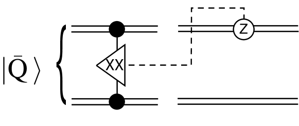
Figure 29: Quantum error correction for $Z$-measurement errors.

Alternatively, a simpler method is shown in fig. 30, where we have $(UV)_{\theta}=(U\otimes V)_{\theta}=\cos\frac{\theta}{2}-i\sin\frac{\theta}{2}\,\,(UV)$ and $(U\otimes V)^{2}={\mathchoice{\rm 1\mskip-4.0mul}{\rm 1\mskip-4.0mul}{\rm 1\mskip-4.5mul}{\rm 1\mskip-5.0mul}}$.

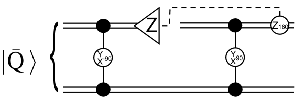
Figure 30: An alternate quantum error correction circuit for $Z$-measurement errors.

Exercise: show that fig. 30 is equivalent to fig. 29, correcting for $Z$-measurement errors on the top qubit.

3.3 Properties of the $Z$-measurement QECC

3.3.1 State Preparation

If we start with the state $|{\psi}\rangle=\alpha|{0}\rangle_{q}+\beta|{1}\rangle_{q}$, how can we prepare the state $|{\bar{\psi}}\rangle=\alpha|{\bar{0}}\rangle+\beta|{\bar{1}}\rangle$? To do this we need an ancilla $|{0}\rangle_{q}$ state, two single qubit rotations and one two qubit rotation, as seen in fig. 31.

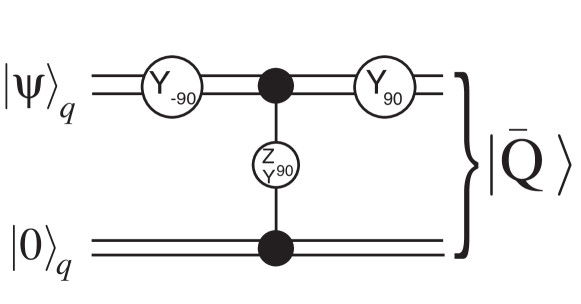
Figure 31: State preparation for the $Z$-measurement code.

Exercise: what single qubit rotations are needed to make $ZZ_{90}$ from a $ZY_{90}$? Note that depending on the choice of $\alpha$ and $\beta$ we can prepare the encoded eigenstates of $X$, $Y$ and $Z$. $X$, $Y$ and $Z$ eigenstate production are error free. Exercise: check that fig. 31 performs the desired transformation on $\alpha|{0}\rangle_{q}+\beta|{1}\rangle_{q}$.

3.3.2 Single qubit rotations

How do we perform encoded $X$, $Y$ and $Z$ operations? It is to verify that the following operators indeed perform the desired operations:

$$\overline{X} = X^{(1)}\,\,(\text{or}\,\,X^{(2)})$$

$$\overline{Y} = Y^{(1)}Z^{(2)}\,\,(\text{or}\,\,Z^{(1)}Y^{(2)})$$

$$\overline{Z} = Z^{(1)}Z^{(2)}\,\,(\text{or}\,\,-Y^{(1)}Y^{(2)})$$

Exercise: check this.

Any single qubit rotation can be made from $X_{\phi}$ and $Z_{90}$ (where $U_{\theta}=\cos\frac{\theta}{2}-i\sin\frac{\theta}{2}\,\,U$ and $U^{2}={\mathchoice{\rm 1\mskip-4.0mul}{\rm 1\mskip-4.0mul}{\rm 1\mskip-4.5mul}{\rm 1\mskip-5.0mul}}$). Exercise: show this by showing how to make $Y_{\phi}$ from $X_{\phi}$ and $Z_{90}$.

The operator $\overline{X}_{\phi}$ is implemented as follows:

$$\overline{X}_{\phi}=\cos{\frac{\phi}{2}}-i\sin\frac{\phi}{2}\overline{X}=\cos{\frac{\phi}{2}}-i\sin\frac{\phi}{2}X^{(1)}I^{(2)}=X^{(1)}_{\phi}I^{(2)}$$

The operator $\overline{Z}_{90}$ is implemented as follows:

$$\overline{Z}_{90}=\frac{1}{\sqrt{2}}(I-i\overline{Z})=\frac{1}{\sqrt{2}}(I-iZ^{(1)}Z^{(2)})=(Z^{(1)}Z^{(2)})_{90}$$

The $(Z^{(1)}Z^{(2)})_{90}$ operation is closely related to the CSign as can be seen in fig. 32. We will show later that teleportation techniques can be used for this gate as it is not error free.

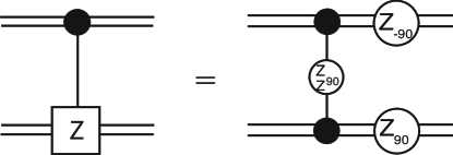
Figure 32: The equivalence between the CSign and $(Z^{(1)}Z^{(2)})_{90}$ operation.

The $Z_{\pm 90}$ gates can be implemented from error free (in our present model) single qubit rotations.

3.3.3 Measurements

After our qubits have been encoded with the code words from eqs. (33) and (34), how do we measure in a particular encoded basis?

To measure in the encoded $\bar{Z}$ eigenbasis: measure both qubits in the $Z$ eigenbasis. The encoded states $|{\bar{0}}\rangle$ and $|{\bar{1}}\rangle$ are distinguished by the parity of the qubits. This can be done error free. To measure in the $\bar{Y}$ basis we need to rotate the qubit using a $X_{90}$ rotation, and then measure in the $Z$ basis as mentioned above. This again can be done error free. If we wanted to measure in the $\bar{X}$ basis, we would need to first rotate the qubits using a $\bar{Y}_{90}$. This rotation, in term of the bare qubits, requires a $YZ_{90}$ gate and cannot be done error free, it will require a CSign gate and thus a chance of an error.

3.3.4 Two qubit rotations

In order to have a universal set of encoded operations we need an encoded entangling operation. The $(\overline{Z}\overline{Z})_{90}$ rotation suffices for this. This can be used to make an encoded CNOT, as shown in fig. 32.

$$(\bar{Z}\bar{Z})_{90} = \frac{1}{\sqrt{2}}(1-i\bar{Z}\bar{Z})$$

$$= \frac{1}{\sqrt{2}}(1-iZ^{(1)}Z^{(2)}Z^{(3)}Z^{(4)})$$

$$= (Z^{(1)}Z^{(2)}Z^{(3)}Z^{(4)})_{90}$$

The circuit to implement $(\overline{Z}\overline{Z})_{90}$ is given in fig. 33. Exercise: confirm this.

Unfortunately fig. 33 does not readily yield a logical gate with significantly less error than using the large entangled states $|{t_{n}}\rangle$ shown in the last section. To do this requires teleportation techniques, as will be explained in the following subsections.

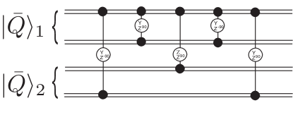
Figure 33: A $(\bar{Z}\bar{Z})_{90}$ gate between qubits $|{\overline{Q}}\rangle_{1}$ and $|{\overline{Q}}\rangle_{2}$.

3.4 Summary so far

With linear optics we can use teleportation along with the large entangled states $|{t_{n}}\rangle$ to perform two qubit operations at the expense of having $Z$-measurement errors. Without correcting for these $Z$-measurement errors the probability scales as $\frac{n}{n+1}$.

To correct for these errors we use the encoding $|{\overline{0}}\rangle=\frac{1}{\sqrt{2}}\bigl{(}|{00}\rangle_{q}+|{11}\rangle_{q}\bigr{)}$ and $|{\overline{1}}\rangle=\frac{1}{\sqrt{2}}\bigl{(}|{01}\rangle_{q}+|{10}\rangle_{q}\bigr{)}$. Encoded $X$, $Y$ and $Z$ eigenstate preparations are error free as are encoded $Y$ and $Z$ measurements.

We can perform encoded operations on this code. $\overline{X}_{\phi}$ is error free however $\overline{Z}_{90}$ requires a two qubit gate so is not. Similarly $(\overline{Z}\overline{Z})_{90}$ is not error free.

3.5 Threshold for $Z$-measurement QECC

3.5.1 Accuracy threshold Theorem

An implementation of information processing is scalable if the implementation can realise arbitrarily many information units and operations with fixed accuracy and with physical resource overheads that are polynomial in the number of information units and operations.

Accuracy Threshold Theorem: If the error per gate is less than a threshold, then it is possible to efficiently quantum compute arbitrarily accurately.

This theorem can be proved by designing fault tolerant gates so that the error model of the encoded gates is the same as the one of the bare qubits. Then we need to concatenate these gates. If the error per qubit at one level of encoding is be less than the error per qubit at the next level of encoding we can keep this concatenation and reduce the effective error rate.

3.5.2 Nice teleportation

In order to understand how to reach a threshold for quantum error correction in LOQC we need to first consider the “nice” teleportation circuit, shown below in fig. 34. The reason why this circuit is “nice” is because of how it effects the quantum information when there is an unintentional measurement error.

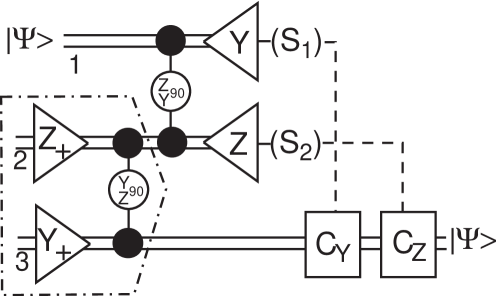
Figure 34: A nice teleportation circuit. The state produced in the dotted-dashed box is $|{tx_{2}}\rangle=\frac{1}{2}\bigl{(}|{00}\rangle_{q}+i|{01}\rangle_{q}+|{10}\rangle_{q}-i|{11}\rangle_{q}\bigr{)}$.

We want to teleport the state $\bigl{(}\alpha|{0}\rangle_{q}+\beta|{1}\rangle_{q}\bigr{)}_{1}$. The action of the correction gates $C_{Y}$ and $C_{Z}$ for each combination of $S_{1}$ and $S_{2}$ are given below:

$S_{1}$	$S_{2}$	$C_{y}$	$C_{z}$
$-1$	$-1$	${\mathchoice{\rm 1\mskip-4.0mul}{\rm 1\mskip-4.0mul}{\rm 1\mskip-4.5mul}{\rm 1\mskip-5.0mul}}$	${\mathchoice{\rm 1\mskip-4.0mul}{\rm 1\mskip-4.0mul}{\rm 1\mskip-4.5mul}{\rm 1\mskip-5.0mul}}$
$+1$	$-1$	$Z$	${\mathchoice{\rm 1\mskip-4.0mul}{\rm 1\mskip-4.0mul}{\rm 1\mskip-4.5mul}{\rm 1\mskip-5.0mul}}$
$-1$	$+1$	${\mathchoice{\rm 1\mskip-4.0mul}{\rm 1\mskip-4.0mul}{\rm 1\mskip-4.5mul}{\rm 1\mskip-5.0mul}}$	$X$
$+1$	$+1$	$Z$	$X$

Exercise: confirm that if we measure

$$|{Y^{+}}\rangle_{1}|{Z^{+}}\rangle_{2} \bigl{(}\alpha|{1}\rangle_{q}-\beta|{0}\rangle_{q}\bigr{)}_{3}$$ we get

$$|{Y^{+}}\rangle_{1}|{Z^{-}}\rangle_{2} \bigl{(}\alpha|{0}\rangle_{q}-\beta|{1}\rangle_{q}\bigr{)}_{3}$$ we get

$$|{Y^{-}}\rangle_{1}|{Z^{+}}\rangle_{2} \bigl{(}\alpha|{1}\rangle_{q}+\beta|{0}\rangle_{q}\bigr{)}_{3}$$ we get

$$|{Y^{-}}\rangle_{1}|{Z^{-}}\rangle_{2} \bigl{(}\alpha|{0}\rangle_{q}+\beta|{1}\rangle_{q}\bigr{)}_{3}$$ we get

before the correction gate.

If an error occurs during the $Y^{(2)}Z^{(3)}_{90}$ state preparation gate, we just try again as they do not corrupt the quantum information. When we consider errors we need to analyse the effect of an unintended $Z$ measurement error on qubit 1 and the effect of an unintended $Y$ measurement error on qubit 2 [23].

The motivation behind looking at unintended $Z$ and $Y$ measurement errors can be seen by looking at the relationship between CSign and the $ZY_{90}$ gate. First consider a CSign gate. As we saw in section 3.1, when we use teleportation to implement a CSign gate it can fail with either a $Z$-measurement error on qubit 1 or a $Z$-measurement error on qubit 2, as seen in fig. 35.

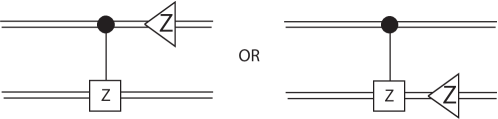
Figure 35: Errors that can result from the teleported CSign gate.

Now consider how these unintentional $Z$-meansurement errors change when we look at the $ZY_{90}$ gate. Exercise: using figs. 10 and 32 show that CSign and $ZY_{90}$ are related as shown in fig. 36.

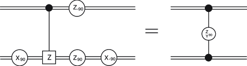
Figure 36: Relation between CSign (Control-Z) and $ZY_{90}$.

Tracing back the potential failures of the $ZY_{90}$ gate due to our error model using figure 36, we get that they can originate from a failure of the CSign gate on the first (control) qubit, leading to a projection in the $Z$ basis or they can originate from a failure of the CSign gate on the second (target) qubit, leading to a projection in the $Y$ basis. And, again, this includes the knowledge of which qubit has failed (as we know this for the CSign gate). Thus the error model after the teleportation is similar to the error model for the unencoded qubits.

In more detail, consider the case of a $Z$ measurement error on qubit 1 in fig. 34.

We need to first work out what the state looks like at point $A$ in fig. 37:

$$\frac{1}{\sqrt{2}}\Bigl{(}i\alpha|{001}\rangle_{q}+\alpha|{010}\rangle_{q}+\beta|{100}\rangle_{q}-i\beta|{111}\rangle_{q}\Bigr{)}_{123}$$ (36)

If we measure qubit 1 in the $Z$ basis we have

$$|{Z^{+}}\rangle_{1}\Bigl{(}i\alpha|{01}\rangle_{q} + \alpha|{10}\rangle_{q}\Bigr{)}_{23}$$

or

$$|{Z^{-}}\rangle_{1}\Bigl{(}i\beta|{00}\rangle_{q} + \beta|{11}\rangle_{q}\Bigr{)}_{23}$$

If this error does occur, our quantum information is corrupted and the gate failed. The failure mode is again a projection in the $Z$ basis.

Next consider that we have a $Y$ measurement error on qubit 2 in fig. 34.

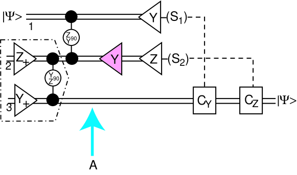
Figure 37: Teleportation with a $Y$-measurement error on qubit 2.

Once again the state at point A in fig. 37 is given by eq. (36). If we measure qubit 2 in the $Y$ basis we have

$$|{Y^{+}}\rangle_{2}\Bigl{(}i\alpha|{01}\rangle_{q}-i\alpha|{00}\rangle_{q}+\beta|{10}\rangle_{q}-\beta|{11}\rangle_{q}\Bigr{)}_{13} = |{Y^{+}}\rangle_{2}\Bigl{(}-i\alpha|{0}\rangle_{q}+\beta|{1}\rangle_{q}\Bigr{)}_{1}\Bigl{(}|{0}\rangle_{q}-|{1}\rangle_{q}\Bigr{)}_{3}$$

or

$$|{Y^{-}}\rangle_{2}\Bigl{(}i\alpha|{01}\rangle_{q}+i\alpha|{00}\rangle_{q}+\beta|{10}\rangle_{q}+\beta|{11}\rangle_{q}\Bigr{)}_{13} = |{Y^{-}}\rangle_{2}\Bigl{(}i\alpha|{0}\rangle_{q}+\beta|{1}\rangle_{q}\Bigr{)}_{1}\Bigl{(}|{0}\rangle_{q}+|{1}\rangle_{q}\Bigr{)}_{3}$$

If this error does occur, our quantum information can be recovered and we can re-use qubit 1 for teleportation.

3.5.3 Teleportation with error recovery

Now say we have an encoded qubit $\alpha|{\overline{0}}\rangle+\beta|{\overline{1}}\rangle$ that experiences a $Z$-measurement error on qubit 1. We saw in fig. 30 that we could correct for the error. When we teleport each part of the encoded qubit and then correct for the $Z$-measurement error on qubit 1 we have:

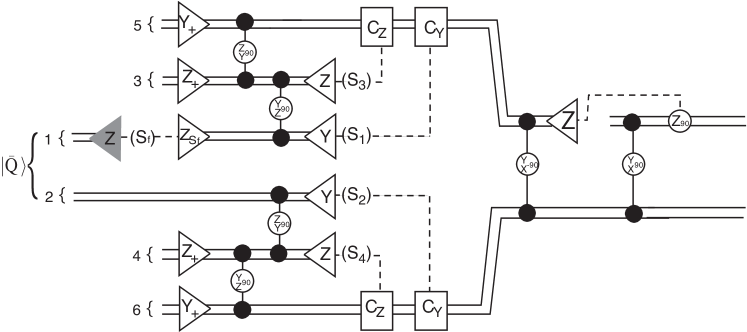
Figure 38: Correcting for $Z$-measurement error on qubit 1.

We can commute the $(Y^{(1)}X^{(2)})_{-90}$, measurement and $(Y^{(1)}X^{(2)})_{90}$ gates to the state production stage, shown in fig. 39.

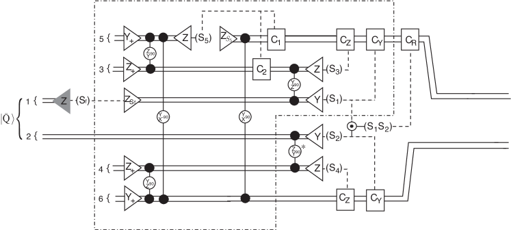
Figure 39: Correcting for $Z$-measurement error on qubit 1 with the error correcting rotations commuted to the state preparation stage.

Exercise: how are the corrections $S_{1}$, $S_{2}$, $S_{3}$ and $S_{4}$ modified after the $(Y^{(1)}X^{(2)})_{-90}$ and $(Y^{(1)}X^{(2)})_{90}$ are commuted through?

We take $f$ to be the probability that teleportation fails. We want to calculate the probability of network 39 to fail: $F_{r}$. We can assume the state preparation has succeeded as it is done offline. We have to look at the modes of failure for the $(Z^{(2)}Y^{(4)})_{90}$ gate (marked with an asterisk, $*$) after the state preparation. First we have a term for the probability that qubit 4 will be projected in the $Y$ basis (which fails with a probability of $f$), which can be undone, and we retry the whole circuit (retrying fails with a probability of $F_{r}$) and thus we get $fF_{r}$. Next we have the probability that the $Y$ projection of qubit 4 succeeds $(1-f)$ but qubit 2 is projected into the $Z$ basis $(f)$ and the circuit fails: $(1-f)f$. We therefore have

$$F_{r}=fF_{r}+(1-f)f\to F_{r}=f,$$ (37)

i.e. the probability of this circuit failing is the same as the probability that the teleportation fails which is the same as the corruption of one of the qubits in the CSign gate.

3.5.4 Encoded $Z_{90}$ Gate

Remember that the encoded $Z_{90}$ gate is given by: $\overline{Z}_{90}=(Z^{(1)}Z^{(2)})_{90}$. As with the error correction after teleportation circuit (figs. 38 and 39), we can commute the $(Z^{(1)}Z^{(2)})_{90}$ back to the state preparation stage, as shown in fig. 40.

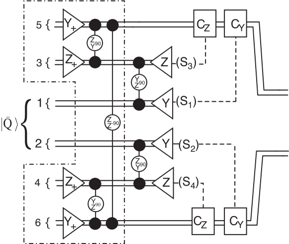
Figure 40: An encoded $Z_{90}$ gate: $\overline{Z}_{90}=(Z^{(1)}Z^{(2)})_{90}$.

We want to calculate the total probability of failure of recovery ($F_{z}$) for this circuit. The probability that both teleportations fail is $f^{2}$. That is, the probability that both qubits 1 and 2 are projected into the $Z$ basis is $f^{2}$. The probability that one qubit is successfully teleported but the other is not, and recovery fails, is $(1-f)f^{2}$. That is, the probability that the top teleportation succeeds and qubit 4 is projected in the $Y$ basis and recovery fails with a projection of qubit 2 in the $Z$ basis is $(1-f)f^{2}$. The probability that one teleportation succeeds but not the other, recovery succeeds and we re-attempt, is $(1-f)fF_{z}$. That is, the probability that the top teleportation succeeds and qubit 4 is projected in the $Y$ basis and recovery succeeds, so we retry the entire circuit is $(1-f)fF_{z}$. We therefore have

$$F_{z}=f^{2}+(1-f)f^{2}+f(1-f)F_{z}\to F_{z}=\frac{2f^{2}-f^{3}}{1-f+f^{2}}$$ (38)

and when the teleporation fails, the mode of error is a projection in the $Z$ basis.

In order to reduce the probability of failure one would perform the teleportations sequentially. To perform $(\bar{Z}\bar{Z})_{90}=(Z^{(1)}Z^{(2)}Z^{(3)}Z^{(4)})_{90}$ we would simply have the same circuit with two more copies of $|{tx_{2}}\rangle$. A similar result for $F_{zz}$ is obtained [23].

3.5.5 Threshold

As mentioned earlier, the error per qubit for one level of concatenation must be less than that for the next level up. In our case, the error for the $ZZ_{90}$ (or Control-sign gate), $f$, must be equal to the error for the next level of encoding, $F_{zz}$ (which is equivalent to $F_{z}$). If we plot $F_{zz}$ vs $f$, we see that $F_{z}=f$ when $f=\frac{1}{2}$, as can be seen in fig. 41. Thus to ensure that the fault tolerant error correction procedure reduces the error probability we need $f<\frac{1}{2}$.

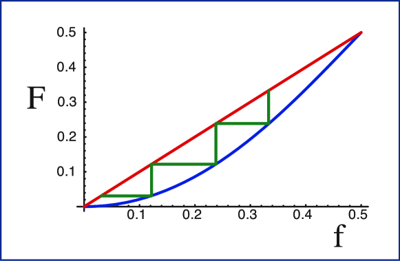
Figure 41: Shows $F=f$ and $F=\frac{2f^{2}-f^{3}}{1-f+f^{2}}$ on the same axis to show the threshold of $f<\frac{1}{2}$.

3.6 Other Errors

So far we have only considered errors due to incorrect measurements at the teleportation stage. There are many other types of errors that may also be important, such as phase errors, inefficient sources, mode absorption/dispersion, imperfect beam splitters, inefficient detectors, $\ldots$ We will consider inefficient detector errors in the next subsection.

3.6.1 Photon Loss

In the original LOQC paper [9], a modification to the gate teleportation protocol was shown that allowed for the detection of photon loss, as shown in fig. 42.

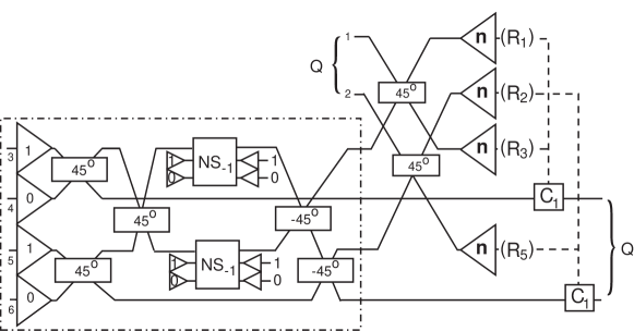
Figure 42: Teleportation with loss detection.

Without going through this circuit explicitly, we know where photon loss occurs through the measurement of ancilla modes. An alternate way to consider loss in teleportation is to say the qubit being teleported is fully “erased”, undergoing the transformation [25]

$$E(\rho)=\frac{1}{4}\bigl{(}\rho+X\rho X+Z\rho Z+Y\rho Y\bigr{)}$$

where $X,Y$ and $Z$ are the usual Pauli operators. This can be considered to be the depolarising channel conditioned on perfect information about which qubit is randomised. Consider we have two state teleportations with the state preparation modified to perform a CSign gate as in fig. 43.

We want to consider what happens if we find photon loss on the top teleporation (for the moment assume there are no $Z$ measurement errors from the teleportation). The top qubit is fully erased, total information is lost. But what about the bottom qubit being teleported?

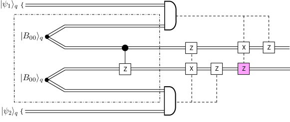
Figure 43: A CSign gate with one of the correction gates applied at the incorrect time.

Because the top qubit is completely randomised, when we perform the gate corrections dependent on the top Bell measurement, the $Z$ gate (in colour in fig. 43) will be applied at the incorrect time. So any photon loss on the top teleportation translates to a full erasure of that qubit being teleported and a $Z$ erasure of the bottom qubit:

$$Z(\rho)=\frac{1}{2}\bigl{(}\rho+Z\rho Z\bigr{)}$$

To correct for erasures we can use the 7-qubit code. This has the stabilzer generators:

$$\begin{array}[]{ccccccccccccl}X&\otimes&X&\otimes&X&\otimes&X&\otimes&{\mathchoice{\rm 1\mskip-4.0mul}{\rm 1\mskip-4.0mul}{\rm 1\mskip-4.5mul}{\rm 1\mskip-5.0mul}}&\otimes&{\mathchoice{\rm 1\mskip-4.0mul}{\rm 1\mskip-4.0mul}{\rm 1\mskip-4.5mul}{\rm 1\mskip-5.0mul}}&\otimes&{\mathchoice{\rm 1\mskip-4.0mul}{\rm 1\mskip-4.0mul}{\rm 1\mskip-4.5mul}{\rm 1\mskip-5.0mul}}\\ X&\otimes&X&\otimes&{\mathchoice{\rm 1\mskip-4.0mul}{\rm 1\mskip-4.0mul}{\rm 1\mskip-4.5mul}{\rm 1\mskip-5.0mul}}&\otimes&{\mathchoice{\rm 1\mskip-4.0mul}{\rm 1\mskip-4.0mul}{\rm 1\mskip-4.5mul}{\rm 1\mskip-5.0mul}}&\otimes&X&\otimes&X&\otimes&{\mathchoice{\rm 1\mskip-4.0mul}{\rm 1\mskip-4.0mul}{\rm 1\mskip-4.5mul}{\rm 1\mskip-5.0mul}}\\ X&\otimes&{\mathchoice{\rm 1\mskip-4.0mul}{\rm 1\mskip-4.0mul}{\rm 1\mskip-4.5mul}{\rm 1\mskip-5.0mul}}&\otimes&X&\otimes&{\mathchoice{\rm 1\mskip-4.0mul}{\rm 1\mskip-4.0mul}{\rm 1\mskip-4.5mul}{\rm 1\mskip-5.0mul}}&\otimes&X&\otimes&{\mathchoice{\rm 1\mskip-4.0mul}{\rm 1\mskip-4.0mul}{\rm 1\mskip-4.5mul}{\rm 1\mskip-5.0mul}}&\otimes&X\\ Z&\otimes&Z&\otimes&Z&\otimes&Z&\otimes&{\mathchoice{\rm 1\mskip-4.0mul}{\rm 1\mskip-4.0mul}{\rm 1\mskip-4.5mul}{\rm 1\mskip-5.0mul}}&\otimes&{\mathchoice{\rm 1\mskip-4.0mul}{\rm 1\mskip-4.0mul}{\rm 1\mskip-4.5mul}{\rm 1\mskip-5.0mul}}&\otimes&{\mathchoice{\rm 1\mskip-4.0mul}{\rm 1\mskip-4.0mul}{\rm 1\mskip-4.5mul}{\rm 1\mskip-5.0mul}}\\ Z&\otimes&Z&\otimes&{\mathchoice{\rm 1\mskip-4.0mul}{\rm 1\mskip-4.0mul}{\rm 1\mskip-4.5mul}{\rm 1\mskip-5.0mul}}&\otimes&{\mathchoice{\rm 1\mskip-4.0mul}{\rm 1\mskip-4.0mul}{\rm 1\mskip-4.5mul}{\rm 1\mskip-5.0mul}}&\otimes&Z&\otimes&Z&\otimes&{\mathchoice{\rm 1\mskip-4.0mul}{\rm 1\mskip-4.0mul}{\rm 1\mskip-4.5mul}{\rm 1\mskip-5.0mul}}\\ Z&\otimes&{\mathchoice{\rm 1\mskip-4.0mul}{\rm 1\mskip-4.0mul}{\rm 1\mskip-4.5mul}{\rm 1\mskip-5.0mul}}&\otimes&Z&\otimes&{\mathchoice{\rm 1\mskip-4.0mul}{\rm 1\mskip-4.0mul}{\rm 1\mskip-4.5mul}{\rm 1\mskip-5.0mul}}&\otimes&Z&\otimes&{\mathchoice{\rm 1\mskip-4.0mul}{\rm 1\mskip-4.0mul}{\rm 1\mskip-4.5mul}{\rm 1\mskip-5.0mul}}&\otimes&Z\end{array}$$

This code can correct for any combination of 1 or 2 erasures and 28 of the possible 35 combinations of 3 erasures. Some of the combinations of 4 erasures can also be corrected. To recover from an erasure of a qubit in an unknown location we would have to measure all six generators.

We always know the location of the erasure, reducing the number of generators to measure down to 2. The 7-qubit code can also correct for $Z$ erasures and $Z$-measurement errors. This is because a $Z$ erasure on a particular qubit is equivalent to an unintentional $Z$ measurement on the qubit of unknown outcome: $Z_{+}\rho Z_{+}+Z_{-}\rho Z_{-}=\frac{1}{2}\bigl{(}{\mathchoice{\rm 1\mskip-4.0mul}{\rm 1\mskip-4.0mul}{\rm 1\mskip-4.5mul}{\rm 1\mskip-5.0mul}}+Z\rho Z\bigr{)}$, where $Z_{\pm}=\frac{1}{2}\bigl{(}{\mathchoice{\rm 1\mskip-4.0mul}{\rm 1\mskip-4.0mul}{\rm 1\mskip-4.5mul}{\rm 1\mskip-5.0mul}}\pm Z\bigr{)}$. In this case only 1 generator needs to be measured. The circuit for this recovery is shown in fig. 44 [25].

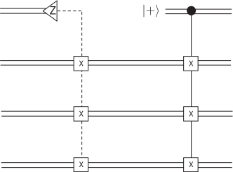
Figure 44: A recovery from a $Z$ erasure or $Z$ measurement error on the top qubit. All other qubits must be erasure free in this case. The remaining 3 qubits in the 7 qubit code are not shown.

In order to estimate how good photon detectors need to be, we estimate the threshold for fault tolerant computation. The gate error threshold was found by Silva et. al. [25] to be bounded below by a value between $1.78\%$ and $11.5\%$. $1.78\%$ results from errors due to loss and $11.5\%$ results from $Z$ measurement errors in teleportation.

4 Conclusion

In these set of lectures we have seen how it was possible to make linear optical elements with single photon sources and detectors behave like a quantum computer. A fundamental idea was to use quantum teleportation to implement gates. If we have probabilistic gates, this teleportation can transfer the difficulty of making a gate to the difficulty of making a state. In our case an extra difficulty was that the teleportation would also induce errors, which could be taken care of. The whole process was streamlined by using quantum error correction, the subject of the last section.

The work on linear optics raises interesting questions about what quantum information is and the origin of its power. Linear optical elements by themselves can be simulated efficiently on a classical computer, but when we measure and condition further gates constructed from linear elements, this is not possible anymore. It is somewhat surprising that this condition on classical information becomes so powerful.

In these lectures we have not mentioned the experiments that have demonstrated the first steps towards implementing LOQC. This is a very active and interesting subject that will be left to another set of lectures.

- [1] DiVincenzo D. P., “The Physical Implementation of Quantum Computation”, Fortschr. Phys., 48 (2000) 771-783.
- [2] Walls D. F. and Milburn G. J., Quantum Optics, (Springer-Verlag, Berlin) 1995.
- [3] Scully M. O. and Zubairy M. S., Quantum Optics, (Cambridge University Press, Cambridge) 1997.
- [4] Leonhardt U., Measuring the Quantum State of Light, (Cambridge University Press, Cambridge), 1997.
- [5] Nielsen M. A. and Chuang I. L., Quantum Computing and Quantum Information, (Cambridge University Press) 2000.
- [6] Yamamoto Y., in Proceedings of the Third Asia-Pacific Physics Conference, edited by Yamamoto Y. and Kitagawa M. and Igeta K., (World Scientific, Singapore), 1988.
- [7] Milburn G. J., “Quantum Optical Fredkin Gate”, Phys. Rev. Lett., 62 (1989) 2124-2127.
- [8] Turchette Q. A., Hood C. J., Lange W., Mabuchi H. and Kimble H. J., “Measurement of Conditional Phase Shifts for Quantum Logic”, Phys. Rev, Lett., 75 (1995) 4710-4713.
- [9] Knill E., Laflamme R. and Milburn G. J., “A scheme for efficient quantum computation with linear optics”, Nature, 409 (2001) 46.
- [10] Reck M., Zeilinger A., Bernstein H. J. and Bertani P., “Experimental Realization of Any Discrete Unitary Operator”, Phys. Rev. Lett., 73 (1998) 58-61.
- [11] Cerf N. J., Adami C. and Kwiat P. G., “Optical Simulation of Quantum Logic”, Phys. Rev. A, 57 (1998) R1477-R1480.
- [12] Lütkenhaus N., Calsamiglia J. and Suominen K. -A., “Bell Measurements for Teleportation”, Phys. Rev. A, 59 (1999) 3295-3300.
- [13] DiVincenzo D. P., “Two-bit gates are universal for quantum computation”, Phys. Rev. A, 51 (1995) 1015-1022.
- [14] Bennet C. H., Brassard G., Crépeau C., Jozsa R., Peres A. and Wooters W., “Teleporting an unknown quantum state via dual classical and EPR channels”, Phys. Rev. Lett., 70 (1993) 1895-1899.
- [15] Gottesman D. and Chuang I. L., “Quantum teleportation is a universal computational primitive”, Nature, 402 (1999) 390-392.
- [16] Knill E., “Quantum gates using linear optics and postselection”, Phys. Rev. A, 66 (2002) 052306.
- [17] Knill E., “Bounds on the probability of success of postselected nonlinear sign shifts implemented with linear optics”, Phys. Rev. A, 68 (2003) 064303.
- [18] Scheel S. and Lütkenhaus N., “Upper bounds on success probabilities in linear optics”, quant-ph/0403103
- [19] Myers C. R., Ralph T.C., “LOQC: generating the entangled states”, unpublished internal IQC preprint (2002).
- [20] Franson J. D., Donegan M. M., Jacobs B. C. , “Generation of entangled ancilla states for use in linear optics quantum computing”, Phys. Rev. A, 69 (2004) 52328.
- [21] Knill E., Laflamme R., Ashishkmin A., Barnum H., Viola L. and Zurek W. H., “Introduction to Quantum Error Correction”, quant-ph/0207170
- [22] Gottesman D., Stabilizer Codes and Quantum Error Correction, Ph.D. thesis, (California Institute of Technology, Pasadena, CA) 1997, also available from quant-ph/9705052
- [23] Knill E., Laflamme R. and Milburn G. J., “Thresholds for linear optics quantum computation”, quant-ph/0006120
- [24] Knill E., in “ITP Program on Quantum Information: Entanglement, Decoherence and Chaos ((online), 2001)” , pp. I-V, http://online.itp.ucsb.edu/online/qinfo01
- [25] Silva M., Rötteler M. and Zalka C., “Thresholds for Linear Optics Quantum Computing with Photon Loss at the Detectors”, quant-ph/0502101