Arnol’d Tongues and Quantum Accelerator Modes.

Abstract

The stable periodic orbits of an area-preserving map on the $2-$torus, which is formally a variant of the Standard Map, have been shown to explain the quantum accelerator modes that were discovered in experiments with laser-cooled atoms. We show that their parametric dependence exhibits Arnol’d-like tongues and perform a perturbative analysis of such structures. We thus explain the arithmetical organisation of the accelerator modes and discuss experimental implications thereof.

I Introduction.

Experiments of atoms optics have discovered the new phenomenon of “quantum accelerator modes” Ox99 . A subsequently formulated theoryFGR02 shows that these modes correspond to stable periodic orbits of the formally classical dynamical system, that is defined on the 2-torus by the map:

$$J_{n+1} = J_{n}+2\pi\Omega+{\tilde{k}}\sin(\theta_{n+1})\qquad\qquad\;\mbox{\rm mod}(2\pi)\;,$$

$$\theta_{n+1} = \theta_{n}+J_{n}\qquad\qquad\qquad\quad\qquad\qquad\mbox{\rm mod}(2\pi)\;.$$ (1)

This map is a variant of the Standard Map, to which it reduces for $\Omega=0$, and its periodic orbits will be characterized in this paper by two integers ${\mathfrak{p}},{\mathfrak{m}}$ so that ${\mathfrak{p}}$ is the period and ${\mathfrak{m}}/{\mathfrak{p}}$ is the winding number “in the $J$ direction”. It should be mentioned that (I) does not emerge from the classical limit $\hbar\to 0$ of the atomic dynamics; and also that the quantum accelerator modes are unrelated to the well known accelerator modes of the Standard MapHan84 ; LL92 , because they do not result of multiples of $2\pi$ being accumulated by an orbit as it winds around the torus in the $J$ direction. In fact they also arise of orbits with ${\mathfrak{m}}=0$, and their origin is subtler; we defer the interested reader to Ref.FGR02 . The modes reported in Ox99 correspond to orbits with ${\mathfrak{p}}=1$; however, the theory predicts that also orbits with higher ${\mathfrak{p}}$ should give rise to accelerator modes; and such “higher order” modes were indeed observed in subsequent experimentsOx03 . This opened the way to “accelerator mode spectroscopy”, i.e. systematic classification of modes according to their numbers ${\mathfrak{p}},{\mathfrak{m}}$. Then the question arose, which winding ratios ${\mathfrak{m}}/{\mathfrak{p}}$ correspond to observable modes, and why. The answer to this question has been recently announcedall05 and is presented in full technical detail in the present paper. We show that the accelerator modes bear an analogy to the widely studied mode-locking phenomenon, which is observed in a variety of classical mechanical systemsOtt . This analogy includes important aspects such as the Arnol’d tongues, and the Farey organisation thereof. At the same time, the present problem has significant differences from well known instances of mode-locking in the physical literature, such as, e.g., those which are reducible to the Circle MapJVB84 . These differences stem from the fact that (I) is a non-dissipative (in fact hamiltonian) dynamical system.
In this paper these issues are analyzed in detail, thus providing a backbone for the results announced in all05 . We develop a perturbation theory for the tongues near their vertex, and a heuristic analysis for the “critical region” where they break. Based on such results we describe and explain the Farey-like arithmetical regularities that emerge from classification of the observed quantum modes, and show that such regularities are encoded by the arithmetical process, of constructing suitable sequences of rational approximants to a real number, which is just the gravity acceleration (measured in appropriate units).
Our perturbative analysis exposes a formal relation to the classical Wannier-Stark problem of a particle subject to a constant field plus a sinusoidal field. This relation has quantum mechanical implications, which are discussed in SFGR05 .

This paper consists of two parts. In the 1st of these (sections II,III, IV) we perform analytical and numerical analysis of the tongues. Based on these results, in the 2nd part (section V) we turn to connections to experiments. The most technical aspects are deferred to Appendices.

II Phase Diagram.

The “phase diagram” in Fig.1 shows the regions of existence of several stable periodic orbits with different ${\mathfrak{p}},{\mathfrak{m}}$ in the plane of the parameters $\Omega,{\tilde{k}}$. The origin of stable periodic orbits of (I) associated with any couple ${\mathfrak{p}},{\mathfrak{m}}$ of mutually prime integers is easily understood. For rational $\Omega={\mathfrak{m}}/{\mathfrak{p}}$ and ${\tilde{k}}=0$, the map has circles of period-${\mathfrak{p}}$ points. As generically predicted by the Poincaré-Birkhoff argument LL92 , at nonzero $\tilde{k}$ these circles are destroyed, and yet an even number of period-${\mathfrak{p}}$ points, half of which are stable, survive in their vicinity. At sufficiently small ${\tilde{k}}>0$ such stable periodic orbits exist in whole albeit small intervals of values of $\Omega$ around ${\mathfrak{m}}/{\mathfrak{p}}$. Exactly this fact gives birth to the experimentally observed accelerator modes; indeed, a stable $({\mathfrak{p}},{\mathfrak{m}})$ orbit of (I) with $\Omega$ in the vicinity of ${\mathfrak{m}}/{\mathfrak{p}}$ gives rise to a quantum accelerator mode, whose physical acceleration is proportional to $|\Omega-{\mathfrak{m}}/{\mathfrak{p}}|$ (FGR02 ; see also sect.V). The persistence of a given winding ratio ${\mathfrak{m}}/{\mathfrak{p}}$ in a whole region of the space of parameters ${\tilde{k}},\Omega$ is where an analogy to the “mode locking” may be seen. As shown in Fig.1, near the ${\tilde{k}}=0$ axis these regions (“tongues”) turn out in the shape of wedges, with vertices at $\Omega={\mathfrak{m}}/{\mathfrak{p}},{\tilde{k}}=0$. The wedges exhibit, at their vertex, an angle, and not a cusp, as is instead the case, e.g. with the Circle Map, and with systems that reduce to it due to dissipationtgs . Moving to higher $\tilde{k}$ inside a tongue, the periodic orbit turns unstable, causing the wedge to break and ramify. Bifurcations follow, which give rise to swallow-like structures. Such “critical structures” of different tongues intertwine and overlap in complicated ways. A tongue is usually overlapped by others, even before breaking, so stable orbits with different ${\mathfrak{p}},{\mathfrak{m}}$ coexist; according to numerical computations, such overlaps persist at very small values of $\tilde{k}$, marking one more difference to the usual scenario. It should be noted that higher-period tongues in Fig.1 hide lower-period ones, and this concurs with graphical and numerical resolution in effacing much of the fine structure of the critical regions.

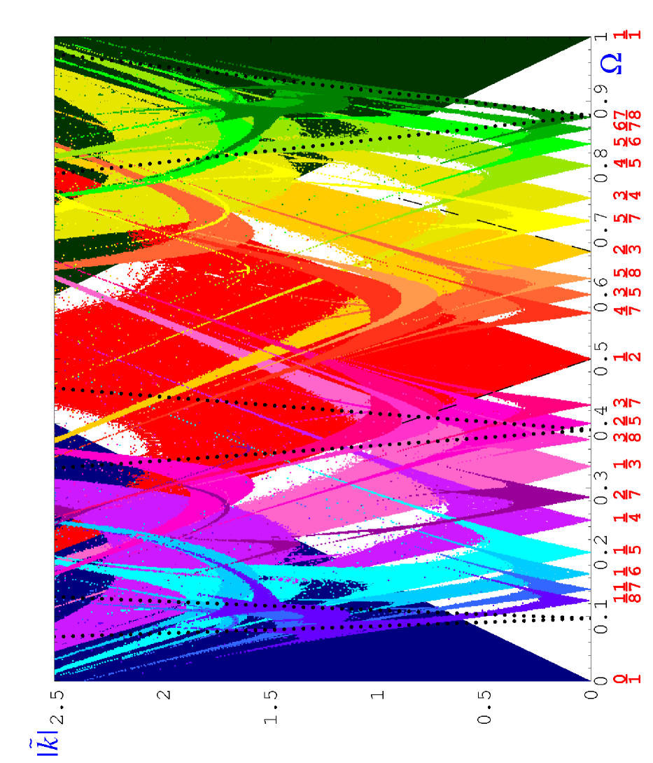
Figure 1: Phase diagram of the map (I), showing the regions of existence and stability (“tongues”) of several periodic orbits with different $({\mathfrak{p}},{\mathfrak{m}})$. The thick dotted black lines represent the locus of the parameter values used in experiments. The dashed black lines show the perturbative theoretical prediction (14) for the margins of a tongue.

III Perturbation theory.

We consider the case when $|{\tilde{k}}|$ is small, and $\Omega$ is close to a rational number ${\mathfrak{m}}/{\mathfrak{p}}$, with ${\mathfrak{m}},{\mathfrak{p}}$ mutually prime integers. We then write

$$\Omega={{\mathfrak{m}}}/{\mathfrak{p}}+\epsilon a\;(2\pi)^{-1}\;\;,\;\;\tilde{k}=\epsilon k\;\;.$$ (2)

where $\epsilon$ is a small parameter. The sign of $a$ and $\epsilon$ is arbitrary, and $k$ may be assumed nonnegative with no limitation of generality. By working out canonical perturbation theory at 1st order in $\epsilon$, we determine the finite angle at the vertex of the ${\mathfrak{p}},{\mathfrak{m}}$ tongue, and obtain an estimate for the area of the stable islands. The whole procedure is an adaptation of Chirikov’s classic analysis Chir , and for $\Omega=0$ our results reproduce well-known ones for the Standard Map.

III.1 Setup.

To open the way to a Hamiltonian formulation, we first of all remove mod$(2\pi)$ from the 1st eqn. in (I) and thereby translate (I) into a map of the cylinder parametrized by $(J,\theta)\in{\mathbb{R}}\times[0,2\pi)$ on itself. Doing so, period-${\mathfrak{p}}$ points on the torus are turned into non-periodic points on the cylinder, due to the constant drift $2\pi{\mathfrak{m}}/{\mathfrak{p}}$ in the 1st eqn. in (I), which is not any more suppressed by mod$(2\pi)$ . For this reason we change variables to $L_{n}\equiv J_{n}-2\pi n{{\mathfrak{m}}}/{\mathfrak{p}}$ and thus obtain:

$$L_{n+1} = L_{n}+\epsilon a\;+\epsilon k\;\,\sin(\theta_{n+1})\;,$$

$$\theta_{n+1} = \theta_{n}+L_{n}+2\pi{{\mathfrak{m}}}n/{\mathfrak{p}}\qquad\qquad\;\;\;\mbox{\rm mod}(2\pi)\;.$$ (3)

This defines a map ${\cal M}_{n}:(L_{n},\theta_{n})\rightsquigarrow(L_{n+1},\theta_{n+1})$ which explicitly depends on the “time” $n$. However, ${\cal M}_{n+{\mathfrak{p}}}={\cal M}_{n}$, so, denoting $L=L_{n{\mathfrak{p}}},\theta=\theta_{n{\mathfrak{p}}}$ and ${\overline{L}}=L_{(n+1){\mathfrak{p}}},{\overline{\theta}}=\theta_{(n+1){\mathfrak{p}}}$, the map ${\cal M}^{({\mathfrak{p}})}:(L,\theta)\rightsquigarrow({\overline{L}},{\overline{\theta}})$ is defined as in

$${\cal M}^{({\mathfrak{p}})} = {\cal M}_{n{{\mathfrak{p}}}+{{\mathfrak{p}}}-1}\circ{\cal M}_{n{{\mathfrak{p}}}+{{\mathfrak{p}}}-2}\circ\ldots\circ{\cal M}_{n{{\mathfrak{p}}}}\;$$ (4)

and does not depend on $n$ any more. The search for period-${\mathfrak{p}}$ points of (I) is thus reduced to search for period-$1$ points of ${\cal M}^{({\mathfrak{p}})}$. For $\epsilon=0$, these fill the circles $L={R_{{\mathfrak{p}},s}}$ , where

$${R_{{\mathfrak{p}},s}}\;\equiv\;\pi(2s-\chi({\mathfrak{p}}))/{\mathfrak{p}}\;\;,\;\;s\in{\mathbb{Z}}\;.$$ (5)

Here $\chi(.)$ is the characteristic function of the even integers. We next write (4) at 1st order in $\epsilon$ in the form of a canonical map that affords implementation of canonical perturbation theory. It is easily seen that, at 1st order in $\epsilon$, the map ${\cal M}^{({\mathfrak{p}})}$ writes:

$${\overline{L}} = L+\epsilon a\;{{\mathfrak{p}}}+\epsilon k\;\sum\limits_{s=1}^{{\mathfrak{p}}}\sin(\theta+sL+\pi{\mathfrak{m}}s(s-1)/{\mathfrak{p}})$$

$$= L+\epsilon a\;{\mathfrak{p}}-\epsilon k\;\frac{\partial}{\partial\theta}G({\mathfrak{p}},{\mathfrak{m}},\theta,L)\;,$$

$${\overline{\theta}} = \theta+{{\mathfrak{p}}}L+\epsilon a\;{{{\mathfrak{p}}}({{\mathfrak{p}}}-1)}/2+\chi({\mathfrak{p}})\pi+\epsilon k\;\sum\limits_{r=1}^{{{\mathfrak{p}}}-1}\sum\limits_{s=1}^{r}\sin(\theta+sL+\pi{\mathfrak{m}}s(s-1)/{\mathfrak{p}})$$ (6)

$$= \theta+{\mathfrak{p}}L+\epsilon a\;{\mathfrak{p}}({\mathfrak{p}}-1)/2+\chi({\mathfrak{p}})\pi+\epsilon k\;(\frac{\partial}{\partial L}-{\mathfrak{p}}\frac{\partial}{\partial\theta})G({\mathfrak{p}},{\mathfrak{m}},\theta,L)\;\;,$$

where

$$G({\mathfrak{p}},{\mathfrak{m}},\theta,L)=\Re\{e^{i\theta}{\mathcal{G}}({\mathfrak{p}},{\mathfrak{m}},L)\}\;\;,\;\;{\mathcal{G}}({\mathfrak{p}},{\mathfrak{m}},L)=\sum\limits_{s=1}^{{\mathfrak{p}}}e^{i\pi{\mathfrak{m}}s(s-1)/{\mathfrak{p}}+isL}\;.$$ (7)

The sums ${\mathcal{G}}({\mathfrak{p}},{\mathfrak{m}},L)$ are a generalized version of the Gauss sums that are studied in number theory. They play an important role in the present problem, and their moduli and arguments will be denoted $A(L)$ and $\xi(L)$ respectively, omitting the specification of ${\mathfrak{p}}$ and ${\mathfrak{m}}$ whenever not strictly necessary. The map (III.1) is not a canonical one, but may be turned canonical, at the cost of higher order corrections only, by replacing $L$ by $\overline{L}$ in the 2nd equation. To show this we note that the function

$$S(\theta,{\overline{L}})=\theta({\overline{L}}-\epsilon a\;{{\mathfrak{p}}})+\chi({\mathfrak{p}})\pi{\overline{L}}+\frac{1}{2}{{\mathfrak{p}}}{\overline{L}}^{2}-\epsilon a\;{\overline{L}}\frac{{{\mathfrak{p}}}({{\mathfrak{p}}}+1)}{2}+\epsilon k\;\,G({\mathfrak{p}},{\mathfrak{m}},{\overline{L}},\theta)$$

generates a canonical transformation $(L,\theta)\to({\overline{L}},{\overline{\theta}})$, given in implicit form by

$${\overline{L}} = L+\epsilon a\;{{\mathfrak{p}}}-\epsilon k\;\frac{\partial}{\partial\theta}G({\mathfrak{p}},{\mathfrak{m}},{\overline{L}},\theta)$$

$${\overline{\theta}} = \theta+{{\mathfrak{p}}}{\overline{L}}+\chi({\mathfrak{p}})\pi-\epsilon a\;{{\mathfrak{p}}}({{\mathfrak{p}}}+1)/2+\epsilon k\;\frac{\partial}{\partial{\overline{L}}}G({\mathfrak{p}},{\mathfrak{m}},{\overline{L}},\theta)\;,$$ (8)

provided that the 1st equation may be uniquely solved for $\overline{L}$. This is indeed the case whenever

$$|\epsilon|<|k|^{-1}c[{\mathfrak{p}}^{3/2}\ln(1+{\mathfrak{p}}/2)]^{-1}\;.$$ (9)

where $c$ is a numerical constant of order unity. This follows from $|\partial_{\overline{L}}{L}-1|\leq|\epsilon k\;\;d{\mathcal{G}}({\mathfrak{p}},{\mathfrak{m}},{\overline{L}})/d{\overline{L}}|$ and from estimate (37) in Appendix VI.3. It is easily seen that replacing $\overline{L}$ by $L$ in the argument of $G$ in (III.1) exactly yields (III.1). As $G$ is scaled by $\epsilon$, this replacement involves an error of higher order than the 1st.

III.2 Resonant approximation.

At 1st order in $\epsilon$, the map (III.1) may be assumed to describe the evolution associated with the time-dependent, “kicked” Hamiltonian

$$H(t)=\frac{1}{2}{{{\mathfrak{p}}}}L^{2}-\epsilon a\;{{{\mathfrak{p}}}}\theta-a\epsilon{{{\mathfrak{p}}}}L/2+\chi({\mathfrak{p}})\pi L+\epsilon k\;G({\mathfrak{p}},{{\mathfrak{m}}},L,\theta)\sum\limits_{n=-\infty}^{\infty}\delta(t-n)\;.$$ (10)

from immediately before one kick to immediately before the next one. This Hamiltonian is a multi-valued function on the cylinder, however multi-valuedness disappears on taking derivatives in the Hamilton equations, and so (10) uniquely determines a ”locally Hamiltonian” flow. We change variable to $L_{0}=L-\epsilon a\;/2$ and drop inessential constants, as well as corrections of higher order in $\epsilon$; and then, in order to remove explicit time dependence, we move into an extended phase space with canonical variables $(\theta,\varphi,L_{0},M_{0})$, and therein consider the time-independent Floquet Hamiltonian :

$$H_{F}(\theta,\varphi,L_{0},M_{0})=\frac{1}{2}{{{\mathfrak{p}}}}L_{0}^{2}+\chi({\mathfrak{p}})\pi L_{0}-\epsilon a\;{{{\mathfrak{p}}}}\theta+2\pi M_{0}+\epsilon k\;G({\mathfrak{p}},{{\mathfrak{m}}},L_{0},\theta)\sum\limits_{m=-\infty}^{\infty}e^{im\varphi}$$ (11)

The variable $\varphi$ is the phase of the periodic driving, and changes in time according to $\varphi(t)=\varphi(0)+2\pi t$. In particular, eqn.(III.1) is obtained with $\varphi(0)=0-$. We consider (11) as a perturbation, scaled by $\epsilon$, of the unperturbed Hamiltonian

$$H_{0}=\frac{1}{2}{{{\mathfrak{p}}}}L_{0}^{2}+\chi({\mathfrak{p}})\pi L_{0}+2\pi M_{0}\;.$$

Points with $L_{0}={R_{{\mathfrak{p}},s}}$ (cp.(5)) and arbitrary $\theta,\varphi,M_{0}$, are fixed under the evolution generated by $H_{0}$ in unit time. For $\epsilon\neq 0$ a 2-parameter family parametrized by $\varphi,M_{0}$ survive near ${R_{{\mathfrak{p}},s}}$. These points may be analyzed by standard methods of classical perturbation theory LL92 in the vicinity of each resonant value ${R_{{\mathfrak{p}},s}}$ of the action $L_{0}$. This calculation is reviewed in Appendix VI.2. The final result is that, for sufficiently small $|\epsilon|$, and near each resonant action ${R_{{\mathfrak{p}},s}}$, the motion in the $L_{0},\theta$ space is canonically conjugate at 1st order in $\epsilon$ to the motion described by the simple Hamiltonian in (12) below. This result is achieved by three subsequent canonical transformations. The first of these removes the oscillating ($\varphi-$dependent) part of the perturbation to higher order in $\epsilon$, except for a “resonant” part, by moving to appropriate new variables $\vartheta_{1},\varphi_{1},L_{1},M_{1}$. The 2nd transformation leads to variables $\vartheta_{2},\varphi_{2},L_{2},M_{2}$ such that the $\theta_{2},L_{2}$ motion is decoupled from the $\varphi_{2},M_{2}$ motion. A final transformation leads to variables $\theta_{3},L_{3}$ such that the 1st order perturbation term in the Hamiltonian depends on the angle variable $\theta_{3}$ alone. The final Hamiltonian is that of a pendulum with an added linear potential:

$$H_{\mbox{\tiny res}}=\frac{1}{2}{\mathfrak{p}}L_{3}^{2}+\epsilon V(\theta_{3})\;\;,\;\;V(\theta_{3})=-{{\mathfrak{p}}}a\theta_{3}+k{\sqrt{\mathfrak{p}}}\cos(\theta_{3})\;\;.$$ (12)

A previous remark about multi-valuedness of (10) applies to this Hamiltonian, too. In spite of being ill-defined on the cylinder, it defines a locally Hamiltonian flow. Replacing the angle $\theta$ by a linear coordinate turns (12) into the Wannier-Stark (classical) Hamiltonian for a particle moving in a line, under the combined action of a constant field and of a sinusoidal static field GKK02 . Relations between the present problem and the Wannier-Stark problem are discussed in SFGR05 .

IV Tongues.

IV.1 Stable fixed points.

Equilibrium (fixed) points $(L_{3}^{*},\theta_{3}^{*})$ of the Hamiltonian (12) must satisfy

$$L_{3}^{*}=0\;\;,\;\;V^{\prime}(\theta_{3}^{*})=-{{\mathfrak{p}}}a-k{\sqrt{\mathfrak{p}}}\sin(\theta_{3}^{*})=0\;,$$ (13)

hence they only exist if $|a|\leq k{\mathfrak{p}}^{-1/2}$, or, equivalently,

$$|\Omega-{{\mathfrak{m}}}/{\mathfrak{p}}|\;\leq\;(2\pi)^{-1}|{\tilde{k}}|\;{\mathfrak{p}}^{-1/2}\;.$$ (14)

Under strict inequality, (13) has two solutions, and one of them is stable. The presence of higher-order corrections, (which were dismissed along the way from (4) to (12)) turns the dynamics from integrable to quasi-integrable, so, assuming a conventional KAM scenario, one may predict a stable orbit of (4) near each resonant action ${R_{{\mathfrak{p}},s}}$, for sufficiently small $|\epsilon|$. In order to determine the equilibrium points in the original variables, one may work backwards the canonical transformations specified in Appendix VI.2 and in the end recall $L=L_{0}+a\epsilon/2$; or else one may directly solve for the fixed points of (III.1) at the 1st order in $\epsilon$. In either case one has to use formulae (34) and (35) in Appendix VI.3. It is then found that

$$L^{*} = R_{{\mathfrak{p}},0}+o(\epsilon)\;\,,\;({\mathfrak{p}}\;\mbox{\rm odd})\;,$$

$$L^{*} = R_{{\mathfrak{p}},0}+\frac{1}{2}a\epsilon+\frac{1}{2}k\epsilon\sin(\theta^{*})+o(\epsilon)\;\;,\;({\mathfrak{p}}\;\mbox{\rm even})\;,$$

$$\theta^{*} = -\arcsin(a\sqrt{{\mathfrak{p}}}/k)-\xi(R_{{\mathfrak{p}},0})+O(\epsilon)\;.$$ (15)

The phases $\xi({R_{{\mathfrak{p}},s}})$ were computed in closed form by number-theoretic means by Hannay and BerryHB80 . A chain of ${\mathfrak{p}}$ fixed points of period ${\mathfrak{p}}$ are then obtained for the original map (I) on the torus. For small $\epsilon$, these points belong to a single primitive periodic orbit of (I), because they result of a continuous displacement, scaled by $\epsilon$, of points in a primitive periodic orbit of (I) for $\epsilon=0$. In the $(\Omega,{\tilde{k}})$ phase diagram, (14) is satisfied in a region bounded by two half-lines originating at ${\tilde{k}}=0,\Omega={\mathfrak{m}}/{\mathfrak{p}}$. At small ${\tilde{k}}$ the half-lines excellently reproduce the side margins of the $({\mathfrak{p}},{\mathfrak{m}})$ tongue, as determined by numerical calculation of the $({\mathfrak{p}},{\mathfrak{m}})$ stable periodic orbits of the exact map (I) (see Fig.5 , and the dashed lines in Fig.1). For ${\mathfrak{p}}=1$ (14) coincides with an exact condition given in FGR02 , which is valid at all $\epsilon$. For ${\mathfrak{p}}>1$ it significantly strengthens that condition, but is only valid at 1st order in $\epsilon$.

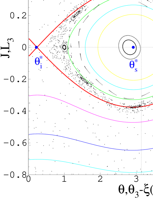
Figure 2: Comparison of the map dynamics (I) with the resonant Hamiltonian dynamics (12) in the vicinity of the resonant action $R_{{\mathfrak{p}},0}=0$, with ${\epsilon a\;}=-0.013$, ${\tilde{k}}=0.1257$, ${\mathfrak{p}}=5$, ${\mathfrak{m}}=2$. The coordinates shown on the axes are $J,\theta$ for the map dynamics (points) and $L_{3},\theta_{3}-\xi(0)$ for the pendulum dynamics (full lines) (cf. eqns.(15)). $\theta^{*}_{i}$ and $\theta^{*}_{s}$ mark the unstable and the stable equilibrium points of (12) respectively; the thick line is the separatrix, and $\theta^{*}_{r}$ marks its return point. These are marked by full circles.

IV.2 Size of perturbative islands.

Elliptic motion around a stable equilibrium point generates a stable island in the $(L_{3},\theta_{3})$ phase space, and hence a stable island for the discrete time motion in the $(J,\theta)$ phase space, with the same area (at 1st order in $\epsilon$). In Fig.2 we show a stable island of the exact map (I) along with a phase portrait of the Hamiltonian flow (12). In the perturbative regime, where the approximation (12) is valid, we roughly estimate the area $\cal A$ of an island by the area enclosed within the separatrix of the integrable pendulum motion (also shown in Fig.2). To this end we introduce a (positive) parameter $\lambda=|a|{\sqrt{\mathfrak{p}}}/k$, so that lines $\lambda=$const. are straight lines through the vertex of the $({\mathfrak{p}},{\mathfrak{m}})$ tongue. The axis of the tongue corresponds to $\lambda=0$ and the side margins to $\lambda=1$, so condition (14) is equivalent to $0\leq\lambda\leq 1$. The estimate is then (see Appendix VI.4):

$${\cal A}\;\approx\;c\;{\mathfrak{p}}^{-1/4}\;|{\tilde{k}}|^{1/2}\;f(\lambda)\;,$$ (16)

where $c$ is some adjustable numerical factor of order unity, slowly varying with $\tilde{k}$ and $\lambda$, and $f(\lambda)$ is an implicit function, defined in Appendix VI.4, the form of which may be inferred from Fig.3. It monotonically decreases from $8\pi$ to $0$ as $\lambda$ increases from $0$ to $1$, and near these endpoints it behaves like:

$$f(\lambda)\; \sim \;8\pi-4(4\pi)^{1/2}\lambda^{1/2}\;\;\mbox{\rm as}\;\;\lambda\to 0+$$

$$f(\lambda)\; \sim \;3^{3/2}\times 2^{7/4}(1-\lambda)^{5/4}\;\;\mbox{\rm as}\;\;\lambda\to 1-\;.$$ (17)

Thus, along lines drawn through the vertex of a tongue, and sufficiently close to the vertex, $\cal A$ decreases proportional to $\sqrt{\tilde{k}}$. The estimate (16) and the asymptotics (IV.2) are well confirmed by direct numerical estimation of areas of stable islands of (I), as shown in Figs 2, 3, 4.

IV.3 Limits of validity.

A crude upper bound for the validity of perturbative analysis is set by overlapping between islands, belonging in the same mode and in neighbouring modes as well. If only the former type of overlapping is considered, then the no-overlap condition reads ${\mathfrak{p}}{\cal A}\lesssim 4\pi^{2}$ and yields $|{\tilde{k}}|\lesssim\;$const.${\mathfrak{p}}^{-3/2}$. Turning estimates based on the overlapping criterion into exact (albeit possibly non-optimal) ones is quite problematic LL92 . However, one may assume that the dependence on the period ${\mathfrak{p}}$ is essentially correct. Two further conditions are set by the validity of (III.1) itself as a $1$st order approximation to (4), which results in the bound (9), and by the validity of the resonant approximation, which results in the bound (31). The logarithmic corrections in (9),(31) are likely to be artifacts of our derivation; in any case, both bounds have nearly the same dependence on the period ${\mathfrak{p}}$ as predicted by the “overlapping criterion”.

IV.4 Crisis of the tongues.

The perturbative estimate (16) is valid near the vertex of a tongue. On further moving upwards in the phase diagram, the area of stable islands first increases up to a maximal value, and then it decreases through strong oscillations (Fig.4). The islands finally disappear, as soon as an upper critical border of stability is reached (Fig.1, Fig.5). On trespassing this border bifurcations are observed FGR02 , giving rise to stable, primitive $({\mathfrak{p}},{\mathfrak{m}})$ orbits, with ${\mathfrak{p}},{\mathfrak{m}}$ non relatively prime. The morphology of tongues in the critical regions where they break is superficially remindful of that observed with other mapsSFK983 and its analysis is outside the scope of this work. In the case ${\mathfrak{p}}=1$, exact non-perturbative calculation of the fixed points and of their stability is possible, showing that the upper stability condition involves the 2nd order in $\epsilon$ FGR02 . Stability thresholds estimated from the trace of the derivative of the map (III.1) at the fixed points miss effects of higher order corrections that were neglected in deriving (III.1) itself from (I). We therefore resort to numerics. Having in mind the border (14) and the discussion in sec.IV.3, we refer each tongue to scaled variables $|{\tilde{k}}|{\mathfrak{p}}^{3/2},|\Omega-{\mathfrak{m}}/{\mathfrak{p}}|{\mathfrak{p}}^{2}$. The horizontal scaling is chosen such that all tongues have the same vertex, and the same angle at their vertex. Fig.5 shows that the subcritical parts of all inspected tongues occupy roughly the same region in the plane of the scaled variables. A similar indication is given by Fig.4. It is worth noting that scaling with the variable ${\mathfrak{p}}^{3/2}|{\tilde{k}}|$ is predicted by (16) for the total area ${\mathfrak{p}}{\cal A}$ of the islands of a period-${\mathfrak{p}}$ orbit, in the perturbative regime of small $\tilde{k}$. On the basis of all such indications we assume that the critical region where a tongue breaks is roughly located around $|{\tilde{k}}_{\mbox{\tiny CR}}|\simeq b\;{\mathfrak{p}}^{-3/2}$, with $b\simeq 6$ as suggested by Figs.5,4. The critical border that way (somewhat vaguely) defined has the same dependence on ${\mathfrak{p}}$ as the previously discussed borders.

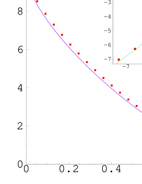
Figure 3: Numerically estimated area of the stable island of the $(1,1)$ orbit of the map (I), at constant $\tilde{k}=0.3666$, as a function of the distance from the centre of the tongue, as measured by the parameter $\lambda=|a|{\mathfrak{p}}^{1/2}/k$ . The full line shows the theoretical estimate (16) , with $c=0.66$. Inset: bilogarithmic magnification of the shaded region near $\lambda=1$. The slope of the dashed line is $5/4$, as predicted by (IV.2).

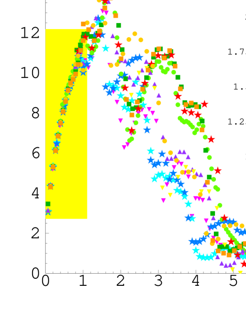
Figure 4: Behaviour of the numerically estimated total area of the chain of stable islands of a periodic orbit, as ${\tilde{k}}$ increases along the line $\lambda=0.1405$ (dotted line in Fig.5). Results are shown for several orbits with periods ${\mathfrak{p}}\leq 18$. Inset: bilogarithmic magnification of the small-${\tilde{k}}$ shaded region. The full line is the perturbative prediction from (16) with $c=0.68$.

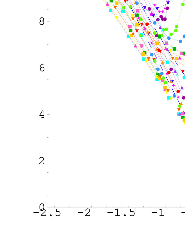
Figure 5: The lower, subcritical parts of tongues of different periods ${\mathfrak{p}}\leq 29$, once rescaled as indicated on the axes, reduce into roughly the same region. The dashed lines show the analytical stability borders of the $(1,0)$ tongue. The dotted line is drawn for reference to Fig.4.

V Spectroscopy of Tongues.

The theory developed in the previous sections provides a quantitative description of the gross structure of the phase diagram. Application to quantum accelerator modes is made in this Section. We first elucidate the physical meaning of the phase diagram in this context.

V.1 Experiments with cold atoms.

In experimentsOx99 ; Ox03 ; ASFG04 , cold caesium atoms of mass $m$ are subject to very short pulses, or “kicks”, with a period $T$ in time. The strength of a kick periodically depends on the position of an atom (assumed to move in a line) at the kicking time, with a period $2\pi/G$ . Its maximal value is denoted $k$. Inbetween kicks, an atom freely falls with the gravitational acceleration $g$. The accelerator modes are observed when $T$ is close to special resonant values, which are given by $T_{\ell}=2\pi\ell m/(\hbar G^{2})$ with $\ell$ any integer. Writing $T=T_{\ell}(1+\epsilon/(2\pi\ell))$, the small parameter $|\epsilon|$ is found to play the formal role of a Planck constant in the quantum equations of motionFGR02 . In the limit when this Planck constant tends to $0$ the atomic dynamics are governed by the “$\epsilon$-classical” map (I), with $2\pi\Omega=GT^{2}g$, ${\tilde{k}}=k\epsilon$ , and $J=n\epsilon$, where $n$ is the atomic momentum measured in units of $\hbar G$ . The theory shows that atoms which are trapped in a stable island of the map move with constant physical acceleration, thereby giving rise to an accelerator mode. Their acceleration relative to that of freely falling atoms is given, in units of $\hbar^{2}G^{3}/m^{2}$, by the parameter $a$ . The acceleration $a$ of a mode may be inferred from the experimental momentum distributions of the atoms after a given number of pulses. As $\Omega$ is known, the rational winding number $r={\mathfrak{m}}/{\mathfrak{p}}$ is then determined. The integers ${\mathfrak{p}}$ and ${\mathfrak{j}}=$sgn$(\epsilon){\mathfrak{m}}$ have been respectively termed the order and the jumping index of a mode FGR02 .

V.2 Quantum Phase Diagram.

At nonzero values of the “Planck constant” $\epsilon$, the $\epsilon$-classical picture is subject to quantal modifications. While the $\epsilon$-classical dynamics only depend on two parameters $\tilde{k},\Omega$, the quantum dynamics additionally depend on the “Planck’s constant” $\epsilon$, which is not determined by ${\tilde{k}}$ and $\Omega$ alone. Thus, for instance, the acceleration $a$ of a mode is not a $\epsilon$-classical variable, because its value at any given point $({\tilde{k}},\Omega)$ in a tongue further depends on $\epsilon$, which is a priori arbitrary. Once a value is chosen for $\epsilon$, the horizontal width of the $({\mathfrak{p}},{\mathfrak{m}})$ tongue at any given value of $\tilde{k}$, multiplied on $\pi/|\epsilon|$, yields the maximal (in absolute value) acceleration that may be attained in the $({\mathfrak{p}},{\mathfrak{m}})$ accelerator mode with the given $\tilde{k}$.
Quantum effects would efface fine structures in the phase diagram, if determined by too small islands compared to $|\epsilon|$. Hence, if a value of $\epsilon\neq 0$ were chosen once and for all, independently of the values of ${\tilde{k}},\Omega$, then high-period tongues would be quantally irrelevant, and low-order modes might be observed only in the inner parts of tongues, sufficiently far from their borders, where the islands shrink to zero. However, in experiments, $\epsilon$ is not fixed, as $\tilde{k}$ is varied by changing $\epsilon$ at constant $k$. As shown by the estimate (16), in this way the area $\cal A$ of an island decreases with $\sqrt{|\epsilon|}$, so the ratio ${\cal A}/|\epsilon|$ grows arbitrarily large at small $\tilde{k}$. Consequently, the $\epsilon$-classical dynamics are more and more accurately reflected in the quantum dynamics of atoms, as the vertex of a tongue is approached. In particular, quantum effects do not set restrictions of principle to the observation of modes of arbitrarily large order. On the contrary, the breakdown of a tongue occurs relatively far from its vertex, and quantum effects may not be negligible there. Significant quantal modifications on the $\epsilon$-classical critical behaviour have been observed and discussed in FGR02 .

V.3 Arithmetics of accelerator modes.

A generic feature of mode-locking phenomena is classification of the locked modes by means of the Farey treeart , which is a standard technique in number theoryNZ960 . This construction is based on a curious propertyfar816 of the irreducible fractions and orders the rational numbers in a hierarchy, which turns out to essentially reproduce the natural hierarchy of the modes, as dictated by their physical “visibility”. In this subsection we discuss the arithmetical organisation of the quantum accelerator modes. To fix ideas, we assume that $\Omega$ ranges in the interval $[0,1]$. For $r$ a rational number in $[0,1]$ we denote ${\mathfrak{m}}(r)/{\mathfrak{p}}(r)$ the corresponding irreducible fraction.

V.3.1 Farey rule.

Due to finiteness of the interaction time, only modes up to some maximal order $M$ can be detected in experiments and in numerical simulations; the integer $M$ being roughly determined by the interaction time . The set ${\cal F}_{M}$ of all rational numbers $r$ such that ${\mathfrak{p}}(r)\leq M$, arranged in increasing order, is known as the $M$-th Farey series. If a rational $r$ is thought of as the winding ratio of an orbit, then ${\cal F}_{M}$ provides a catalog of all the tongues of period $\leq M$, ordered from left to right in the phase diagram. This may be termed the $M$-th Farey family of tongues. If $M>1$, then statements (F1) and (F2) below are true of the Farey series ${\cal F}_{M}$ HW79 :
(F1) If $r_{1}$ and $r_{2}$ with $r_{2}>r_{1}$ are nearest neighbours in the Farey series ${\cal F}_{M}$, then ${\mathfrak{p}}(r_{1}){\mathfrak{m}}(r_{2})-{\mathfrak{p}}(r_{2}){\mathfrak{m}}(r_{1})=1$. In particular, ${\mathfrak{p}}(r_{1})$ and ${\mathfrak{p}}(r_{2})$ are relatively prime integers, and so are ${\mathfrak{m}}(r_{1})$ and ${\mathfrak{m}}(r_{2})$.
(F2) If $r_{3}$ is the element of ${\cal F}_{M}$ that follows $r_{2}$ on the right, then $r_{2}$ is the Farey mediant of $r_{1}$ and $r_{3}$, i.e.:

$$r_{2}=\frac{{\mathfrak{m}}(r_{1})+{\mathfrak{m}}(r_{3})}{{\mathfrak{p}}(r_{1})+{\mathfrak{p}}(r_{3})}$$

These facts have the following consequence. Let two tongues $r_{1},r_{2}$ be “adjacent”, in the sense that no other tongue exist between them, with a period less or equal to the largest of the periods ${\mathfrak{p}}(r_{1}),{\mathfrak{p}}(r_{2})$. Then (F2) implies that the tongue with the smallest period, to be found between them, is the tongue associated with the Farey mediant of $r_{1}$ and $r_{2}$. This may be called the “Farey rule”. A qualitative formulation of this rule is : the next most visible tongue to be observed between two adjacent tongues labeled by rationals $r_{1}$ and $r_{2}$ is the tongue labeled by the Farey mediant of $r_{1}$ and $r_{2}$. This rule does no more than reflect the fact that tongues are the less visible, the higher their period.

V.3.2 Experimental Paths.

Orders and jumping indexes of quantum accelerator modes are identified, by monitoring the atomic momentum distributions that are obtained after a fixed time with different parameter values. The latter are generated by continuously varying a single control parameter: the pulse period $T$ (or, equivalently, $\epsilon$) in ranges close to the resonant values $T_{\ell}$. The locus of the corresponding points in the $({\tilde{k}},\Omega)$ plane is then a continuous curve, that will be termed the Experimental Path (EP) in the following. The problem then arises, of classifying the tongues, that have a significant intersection with a given EP. These are but a small subclass of the Farey family of tongues that fits the given interaction time, because many tongues in that family are met by the EP in their overcritical regions, where islands are typically small, yielding hardly if at all detectable modes. Thus the analysis of observable modes rests on three key facts. The first of these is existence of a critical border (sect.IV.4). Second, an EP hits the ${\tilde{k}}=0$ axis at a value of $\Omega$ given by $\omega=GgT^{2}_{\ell}/(2\pi)$, which corresponds to $\epsilon=0$, or $T=T_{\ell}$. Third, the quantum dynamics grow more and more quasi-$\epsilon$-classical as ${\tilde{k}}=0$ is approached along an EP, and this justifies analysis based on the $\epsilon$-classical phase diagram. These three facts reduce the problem of predicting the observable modes to a number-theoretic problem, of constructing suitable sequences of rational approximants to the real number $\omega$. If space is measured in units of the spatial period of the kicks, and time in units of $T_{\ell}$, then $\omega$ is just the gravity acceleration.
An EP may in general be described by an equation $\Omega=\omega+\Phi({\tilde{k}})$, where $\Phi({\tilde{k}})$ is some strictly monotonic function such that $\Phi(0)=0$. The experiments in Ox03 will be used as a model case in this section, and the corresponding EPs are shown by the black dotted lines in Fig.1 . Each choice of $\ell=1,2,3$ yields an EP consisting of two lines which will be henceforth referred to as the two “arms” of the EP. The left (resp., right) arms of the EPs corresponds to negative (resp., positive) values of $\epsilon$. With $\ell=2$ the arms meet at $\tilde{k}=0,\Omega=\omega\approx 0.390152...$ and are approximately linear at small $\tilde{k}$: $|{\tilde{k}}|\approx\alpha|\omega-\Omega|$, with $\alpha=\hbar^{2}G^{3}k/(2m^{2}\ell g)$; so we may assume $\Phi({\tilde{k}})\approx\alpha^{-1}{\tilde{k}}$ at small values of $\epsilon$ for the case of Fig.1.
Independently of the specific form of $\Phi$, the intersection of an EP with the subcritical $({\mathfrak{p}},{\mathfrak{m}})$ tongue is defined by two conditions, one dictated by (14), and the other by the critical border $|{\tilde{k}}_{\mbox{\tiny crit}}|\simeq b{\mathfrak{p}}^{-3/2}$ with $b\sim 2\pi$:

$$|{\mathfrak{m}}/{\mathfrak{p}}-\Omega|<(2\pi)^{-1}{\mathfrak{p}}^{-1/2}|{\tilde{k}}|\;\;,\;\;|\omega-\Omega|=|\Phi({\tilde{k}})|<|\Phi(2\pi{\mathfrak{p}}^{-3/2})|\;$$ (18)

These inequalities lead to

$$|\omega-{\mathfrak{m}}/{\mathfrak{p}}|<(2\pi)^{-1}b{\mathfrak{p}}^{-2}+|\Phi(2\pi{\mathfrak{p}}^{-3/2})|\simeq{\mathfrak{p}}^{-2}+|\Phi(2\pi{\mathfrak{p}}^{-3/2})|\;,$$ (19)

and show that the winding ratios $r={\mathfrak{m}}/{\mathfrak{p}}$ that are observed along an EP have to approximate $\omega$ the better, the smaller $\epsilon$.

V.3.3 Farey algorithm.

According to (19), the winding ratios of modes oberved along an EP form a sequence of rational approximants to $\omega$. This fact was already noted in FGR02 , and the question arose, which of the densely many rational winding ratios that lie arbitrarily close to $\omega$ are actually observable. The Farey rule may be used to answer this question . Modes are the more visible, the smaller their order; therefore, modes observed on moving along an EP towards $\omega$ should achieve better and better approximations to $\omega$, at the least possible cost in terms of their orders ${\mathfrak{p}}$. Issues of criticality, and of quasi-$\epsilon$-classicality, additionally suggest that, as a thumb rule, modes should be more safely observable near the vertex of their tongues. These indications suggest the following construction. Assuming that $\Omega$ ranges in the interval $[0,1]$, the strongest modes are the period-$1$ ones, $(1,0)$ and $(1,1)$. According to the Farey rule in the end of sect.V.3.1, the next strongest mode is associated with their Farey mediant, $(2,1)=(1+1,0+1)$. At the next step two further Farey mediants $(3,1)=(1+2,0+1)$ and $(3,2)=(1+2,1+1)$ appear. The former is closer to $\omega\approx 0.39...$ than the latter, so its tongue intersects the EP at lower $|\epsilon|$ . It is therefore expected to produce a stronger mode; so we discard $(3,2)$, and restrict to the interval $[1/3,1/2]$. The process may then be iterated. At the $n$-th step, it will have singled out two rationals, $r^{\prime}_{n,\omega}$ and $r^{\prime\prime}_{n,\omega}$, such that the Farey interval $F_{\omega,n}=[r^{\prime}_{n,\omega},r^{\prime\prime}_{n,\omega}]$ contains $\omega$, but does not contain any rational with a divisor smaller than ${\mathfrak{p}}(r^{\prime}_{n,\omega})+{\mathfrak{p}}(r^{\prime\prime}_{n,\omega})$. If $\omega$ is itself a rational, then it is eventually obtained as the Farey mediant of the endpoints of a Farey interval $F_{\omega,n}$, and then the process terminates. The process just described is an arithmetic recursion for generating rational approximants to $\omega$, that will be termed here ”the Farey algorithm”. Out of all possible rational approximants to $\omega$, it selects the endpoints of the Farey intervals of $\omega$, as the winding ratios whose prediction is safer.

V.3.4 Accelerator modes, as Rational Approximants of Gravity.

It is now necessary to discuss consistency of the Farey algorithm with the key condition (19), that dictates the rate at which modes of increasing order ${\mathfrak{p}}$ have to approximate the gravity acceleration $\omega$. This rate depends on the form of the function $\Phi$; however, in no case it is required to be faster than quadratic, thanks to the 1st term on the rhs of (19). For this reason, observation of the principal convergents (or simply the convergents) to $\omega$ is always expected. These are the rationals $s_{\omega,n}$ that are obtained by truncating the continued fraction of $\omega$, and are “best rational approximants” to $\omega$ in the sense that (Thm.182 in HW79 , p.151):

$${\mathfrak{p}}(s_{\omega,n})|\omega-s_{\omega,n}|<{\mathfrak{p}}(r)|\omega-r|\;\;,\;\;\mbox{\rm whenever}\;\;{\mathfrak{p}}(r)<{\mathfrak{p}}(s_{\omega,n})\;.$$ (20)

They are known to satisfy $|\omega-s_{\omega,n}|<{\mathfrak{p}}(s_{\omega,n})^{-2}$, and hence (19) as well, and are in fact clearly detected in experiments and in numerical simulations. The Farey algorithm generates all of the convergents to $\omega$. As shown in Appendix VI.1, at least one endpoint of each Farey interval is a convergent to $\omega$; however, except for quite particular choices of $\omega$, the Farey algorithm generates more approximants than just the convergents, and so a Farey interval generated by the algorithm may have only one endpoint given by a convergent. In that case, that very convergent is also an endpoint of the next generated interval, and possibly of subsequently generated ones, until the construction produces the next convergent at the other endpoint. By construction, $r^{\prime}_{n,\omega}$ is the rational that yields the best approximation from the left in the class of all rationals $r$ with ${\mathfrak{p}}(r)\leq{\mathfrak{p}}(r^{\prime}_{n,\omega})$; and $r^{\prime\prime}_{n,\omega}$ has the the same property in what concerns approximations from the right. The one of the two approximants $r^{\prime}_{n,\omega},r^{\prime\prime}_{n,\omega}$ that lies closer to $\omega$ is called the $n$-th Farey approximant to $\omega$, and will be denoted $r^{*}_{\omega,n}$. It is by construction a best rational approximant to $\omega$, in a weaker sense than (20): notably,

$$|\omega-r^{*}_{\omega,n}|<|\omega-r|\;\;\mbox{\rm whenever}\;\;{\mathfrak{p}}(r)<{\mathfrak{p}}(r^{*}_{\omega,n})\;.$$ (21)

The approximation of $\omega$ which is granted by a Farey approximant may not be quadratic when the approximant is not a convergent; therefore, whether a Farey approximant satisfies condition (19) depends on the form of the function $\Phi$. That condition is the more exacting, the steeper the EP, which is the graph of the function $\Phi$. For instance, in the extreme case when the EP is a vertical line drawn through $\omega$ (which corresponds to $\alpha=\infty$ in our model case ), the 2nd term in (19) is absent and the approximation has to be strictly quadratic. This may rule out some of the non-principal approximants produced by the algorithm, depending on arithmetical properties of $\omega$. For $\omega$ equal to the Golden Ratio, all the Farey endpoints are principal convergents. All the corresponding modes, and none other, were observed in numerical simulations of the atomic dynamics (Fig.6) . For a “less irrational” choice $\omega=\pi-3$, the Farey algorithm generates many other approximants besides the convergents. All those with order ${\mathfrak{p}}\leq 106$ were detected by our numerical simulations of the atomic dynamics up to $800$ pulses, except for two, and these were found to violate (19).
When the EP is not vertical the 2nd term in (19) opens the way to non-quadratic approximants. For the EP we consider here, this term is given by $2\pi\alpha^{-1}{\mathfrak{p}}^{-3/2}$ and prevails over the 1st term at sufficiently large ${\mathfrak{p}}$. For this reason, according to theorem (T6) in Appendix VI.1, for almost all $\omega$ (in the sense of Lebesgue measure), all of the Farey endpoints, except possibly for finitely many exceptions, satisfy (19). Since the 2nd term in (19) prevails over the $1$st the later (that is, at larger ${\mathfrak{p}}$), the steeper the EP, (in our model case, the larger $\alpha$), the possible “finitely many exceptions” may be relevant in the analysis of data, which of necessity cannot extend to arbitrarily large ${\mathfrak{p}}$.
In conclusion, the Farey-based prediction of modes may suffer exceptions, both in the case when the EP is very steep, and in the opposite case when it is very flat, by generating more approximants (in the former case), and less (in the latter case) than allowed by (19). In addition, (19) itself is not exact, as it rests on a coarsely defined critical border. In particular, large fragments of broken tongues, too, may produce significant modes at times.

V.3.5 Final remarks.

Left- and Right-hand Modes. By construction, $r^{\prime}_{\omega,n}$ and $r^{\prime\prime}_{\omega,n}$ approximate $\omega$ from the left and from the right respectively. Therefore, the vertex of the $r^{\prime}_{\omega,n}$ tongue lies on the left of $\omega$, so the intersection of the tongue with the left arm of the EP lies at significantly lower $\tilde{k}$ than its intersection with the right arm; hence, it should be preferably observed at $\epsilon<0$. It is in fact an empirical observation, that left (resp., right) approximants preferably occur at negative (resp., positive) values of $\epsilon$. In particular, two successive convergents to $\omega$ approximate $\omega$ from opposite sides, so the corresponding modes are in principle expected on opposite arms. This is not a strict rule, as tongues with relatively small ${\mathfrak{p}}$ may have significant intersection with both arms of an EP. Some low-period modes could indeed be observed on both arms, and were found to correspond to convergents of $\omega$. However, this cannot happen when the period of a tongue is so large that the slope $2\pi\sqrt{\mathfrak{p}}$ of its margins is larger than the slope of the arm lying on the opposite side with respect to $\omega$. Thus, modes of sufficiently large order should never be expected on both sides. In that case the two arms coincide, so there is complete symmetry between $\epsilon>0$ and $\epsilon<0$, as can be seen in Fig. 6.
The case of rational $\omega$. If $\omega$ is a rational number $r/s$ , then the Farey algorithm eventually terminates. It is therefore expected that, whatever the observation time, only a finite number of modes are observable. This case has been experimentally realized, too Ox04 . The arms of the EP exactly meet at the vertex of the $(s,r)$ tongue. If their slope is larger than $2\pi\sqrt{s}$ (as in Ox04 ) then the $(s,r)$ mode is observed on both arms, and at all values of $|\epsilon|$ below a certain value determined by the critical border of the $(s,r)$ tongue. On the contrary, the $(s,r)$ mode could never be observed if $2\pi\sqrt{s}$ were larger than the slope of the arms.

Figure 6: A Fibonacci sequence of quantum accelerator modes, as revealed by numerically computed momentum distributions of a cloud of $50$ atoms after $400$ pulses, with $k=0.8\pi$, $\Omega=$const.$=\omega=({\sqrt{5}}-1)/2$ (the Golden Mean), and for different values of the kicking period $T=T_{\ell}(1+\epsilon/(2\pi\ell))$ in the vicinity of $T=T_{\ell},\ell=2$. The atomic momentum $n$ is shown on the vertical axis. It is measured in a free-falling frame, and is assumed positive in the direction of gravity. On the horizontal axis $\epsilon$ is replaced by the variable $\epsilon^{*}={\rm sgn}(\epsilon)\sqrt{\mid\epsilon\mid/2\pi}$, which affords relative magnification of the small-$\epsilon$ region. The hyperbola-like zones of enhanced population are the accelerator modes. Their shapes and positions yield access to their winding ratios ${\mathfrak{m}}/{\mathfrak{p}}$ : $(A)$ $2/3$, $(B)$ $3/5$, $(C)$ $5/8$, $(D)$ $8/13$, $(E)$ $13/21$, $(F)$ $21/34$, $(G)$ $34/55$, $(H)$ $55/89$, $(I)$ $89/144$. These are the principal convergents to the Golden Mean. Note the exact symmetry under reflection in the origin of the axes.

VI Appendix.

VI.1 The Farey Algorithm.

What in this paper is termed ”the Farey algorithm” is a recursive means of constructing rational approximants to a given real number $\omega$, by iterated calculation of Farey mediants. Though the role of the Farey properties (F1),(F2) (sect.V.3.1) in the process of rational approximation is a basic notion in the theory of numbersNZ960 , it is not easy to locate references wherein those aspects which are directly used in this paper be presented in a self-contained way. Such a self-contained presentation is given in this Appendix. The one input we use is the Basic Theorem stated below, which is equivalent to properties (F1) and (F2) of the Farey series in sect.V.3.1. Proofs of (F1) and (F2), hence of the basic theorem, may be found, e.g., in ref.HW79 .
Let $\omega\in[0,1]$ be fixed. Given a rational $r\in[0,1]$ we denote ${\mathfrak{m}}(r)/{\mathfrak{p}}(r)$ the corresponding irreducible fraction. We further denote $d_{\omega}(r)=|r-\omega|$ and $\delta_{\omega}(r)={\mathfrak{p}}(r)d_{\omega}(r)$. We say that a rational $r$ is $\delta$-closer to $\omega$ than another rational $s$ if $\delta_{\omega}(r)<\delta_{\omega}(s)$; and we say that $r$ is $d$-closer to $\omega$ than $s$ if $d_{\omega}(r)<d_{\omega}(s)$.
DO:A best rational $d$-approximant (dBA) to $\omega$ is a rational $r$ such that $d_{\omega}(r)<d_{\omega}(s)$ for any rational $s$ with ${\mathfrak{p}}(s)<{\mathfrak{p}}(r)$. Replacing $d$ by $\delta$ yields the definition of a best rational $\delta$-approximant ($\delta$BA) to $\omega$.
The dBAs and the $\delta$BAs to $\omega$ are respectively known as the Farey approximants and the principal convergents to $\Omega$. From the definition it follows that every $\delta$BA is at once a dBA. Another immediate consequence is:
T0: Let $r_{1}$ and $r_{2}$ be two successive dBAs to $\omega$, in the sense that ${\mathfrak{p}}(r_{2})>{\mathfrak{p}}(r_{1})$, and no rational $r$ with ${\mathfrak{p}}(r_{1})<{\mathfrak{p}}(r)<{\mathfrak{p}}(r_{2})$ is a dBA. Then $d_{\omega}(r)\geq d_{\omega}(r_{1})$ for all rational $r$ with ${\mathfrak{p}}(r_{1})<{\mathfrak{p}}(r)<{\mathfrak{p}}(r_{2})$. The statement remains true on replacing $d$ by $\delta$.
D1: A Farey interval is a closed interval with rational endpoints $r^{\prime},r^{\prime\prime}$ ($r^{\prime}<r^{\prime\prime}$) satisfying ${\mathfrak{m}}(r^{\prime\prime}){\mathfrak{p}}(r^{\prime})-{\mathfrak{m}}(r^{\prime}){\mathfrak{p}}(r^{\prime\prime})=1$, or, equivalently, $r^{\prime\prime}-r^{\prime}=1/({\mathfrak{p}}(r^{\prime}){\mathfrak{p}}(r^{\prime\prime}))$.
D2: The Farey mediant of two rationals $r^{\prime},r^{\prime\prime}$ is the rational $r^{\prime}\oplus r^{\prime\prime}\equiv({\mathfrak{m}}(r^{\prime})+{\mathfrak{m}}(r^{\prime\prime}))/({\mathfrak{p}}(r^{\prime})+{\mathfrak{p}}(r^{\prime\prime}))$.

BT (The Basic Theorem): The following statements are equivalent: (a) $F=[r^{\prime},r^{\prime\prime}]$ is a Farey interval, (b) ${\mathfrak{p}}(r)\geq{\mathfrak{p}}(r^{\prime})+{\mathfrak{p}}(r^{\prime\prime})$ holds true of any rational $r$ with $r^{\prime}<r<r^{\prime\prime}$; equality holding if, and only if, $r=r^{\prime}\oplus r^{\prime\prime}$.

Denote ${\cal F}_{\omega}$ the family of all the intervals $F\subseteq[0,1]$ such that $F$ is a Farey interval and $\omega$ is an internal point of $F$. Further define a family of intervals ${\overline{\cal F}_{\omega}}$ so that ${\overline{\cal F}_{\omega}}={\cal F}_{\omega}$ for irrational $\omega$ and ${\overline{\cal F}_{\omega}}={\cal F}_{\omega}\cup\{[\omega]\}$ for rational $\omega$, where $[\omega]$ is a shorthand notation for the interval $[\omega,\omega]$.
If $F=[r^{\prime},r^{\prime\prime}]$ is a Farey interval, then each of the intervals $[r^{\prime},r^{\prime}\oplus r^{\prime\prime}]$, $[r^{\prime}\oplus r^{\prime\prime},r^{\prime\prime}]$ is a Farey interval. One may then define a map ${\mathfrak{F}}_{\omega}:{\overline{\cal F}_{\omega}}\to{\overline{\cal F}_{\omega}}$ as follows. If $F=[r^{\prime},r^{\prime\prime}]\in{\cal F}_{\omega}$ and $r^{\prime}\oplus r^{\prime\prime}\neq\omega$, then ${\mathfrak{F}}_{\omega}(F)$ is the one of the intervals $[r^{\prime},r^{\prime}\oplus r^{\prime\prime}],[r^{\prime}\oplus r^{\prime\prime},r^{\prime\prime}]$ that contains $\omega$. If $F=[r^{\prime},r^{\prime\prime}]\in{\cal F}_{\omega}$ and $r^{\prime}\oplus r^{\prime\prime}=\omega$, then ${\mathfrak{F}}_{\omega}(F)=[\omega]$. Finally ${\mathfrak{F}}_{\omega}([\omega])=[\omega]$. The following proposition shows that the map ${\mathfrak{F}}_{\omega}$ provides an algorithm for recursively generating the whole of ${\overline{\cal F}_{\omega}}$.

T1 (The Farey algorithm) :Let $\omega\in(0,1)$ be given. For integer $n\geq 0$ define $[{r^{\prime}_{\omega,n}},{r^{\prime\prime}_{\omega,n}}]\equiv F_{\omega,n}\equiv{\mathfrak{F}}_{\omega}^{n}([0,1])$. Then:
(a) $\{F_{\omega,n}\}_{n\geq 0}$ is a monotone nonincreasing sequence (in the set theoretical sense) of closed intervals; moreover $\lim_{n\to\infty}|F_{\omega,n}|=0$ and $\cap_{n\geq 0}F_{\omega,n}=[\omega]$,
(b) If $\omega$ is rational then $F_{\omega,n}=[\omega]$ eventually,
(c) $\{F_{\omega,n}\}_{n\geq 0}={\overline{{\cal F}_{\omega}}}$.
Proof: (a) immediately follows from D1, D2, and from the definition of ${\mathfrak{F}}_{\omega}$. (b): if $F_{\omega,n}\neq[\omega]$ then $F_{\omega,n}$ is a Farey interval and contains $\omega$ as an internal point. Due to BT(b), the family of such Farey intervals is finite whenever $\omega$ is rational.
(c): we have to show that $F\in{\overline{\cal F}_{\omega}}$ implies $F=F_{\omega,n}$ for some integer $n$. If $F=[0,1]$ then $F=F_{\omega,0}$, and if $F=[\omega]$ then $\omega$ is rational and the claim follows from (b). Thus we assume $F=[r^{\prime},r^{\prime\prime}]\subset[0,1]$ with $r^{\prime}<r^{\prime\prime}$, and then (a) implies that $F\subset F_{\omega,n}$ can hold only for finitely many values of $n$. Let $N$ be the largest such value. From $F\neq[\omega]$ it follows that $F_{\omega,N}\neq[\omega]$, so $r^{\prime}_{\omega,N}\oplus r^{\prime\prime}_{\omega,N}$ is an endpoint of $F_{\omega,N+1}$, and then $r^{\prime}_{\omega,N}\oplus r^{\prime\prime}_{\omega,N}\in F$ because $F$ is not strictly a subset of $F_{\omega,N+1}$ by the definition of $N$. If $r^{\prime}_{\omega,N}\oplus r^{\prime\prime}_{\omega,N}$ were an internal point of $F$, then BT(b) would imply ${\mathfrak{p}}(r^{\prime}_{\omega,N}\oplus r^{\prime\prime}_{\omega,N})={\mathfrak{p}}(r^{\prime}_{\omega,N})+{\mathfrak{p}}(r^{\prime\prime}_{\omega,N})\geq{\mathfrak{p}}(r^{\prime})+{\mathfrak{p}}(r^{\prime\prime})$ which is impossible because one at least of $r^{\prime}$ and $r^{\prime\prime}$ is an internal point of $F_{\omega,N}$ and so its divisor is not less than ${\mathfrak{p}}(r^{\prime}_{\omega,N}\oplus r^{\prime\prime}_{\omega,N})$. Therefore, $r^{\prime}_{\omega,N}\oplus r^{\prime\prime}_{\omega,N}$ is an endpoint of both $F$ and $F_{\omega,N+1}$. Since the former is not strictly a subset of the latter, and both contain $\omega$, $F=F_{\omega,N+1}$ follows. $\Box$

T2:At least one endpoint of each $F_{\omega,n}$ is a dBA to $\omega$; and every dBA to $\omega$ is an endpoint of some $F_{\omega,n}$.
Proof: Denote $r^{*}_{n}$ the endpoint of $F_{\omega,n}$ that is $d$-closer to $\omega$. No rational with a divisor less than ${\mathfrak{p}}(r^{*})$ lies inside $F_{\omega,n}$ by construction, so $r^{*}_{n}$ is a dBA.
Conversely, let $r$ be a dBA. The claim is obviously true if $r=0$ or $r=1$, so let $r$ lie strictly inside $F_{0}=[0,1]$, and let $m$ be the largest integer such that $r$ is an internal point of $F_{\omega,m}$. Due to BT(b), $m$ is a finite number, and ${\mathfrak{p}}(r)\geq{\mathfrak{p}}(r^{\prime}_{\omega,m})+{\mathfrak{p}}(r^{\prime\prime}_{\omega,_{m}})={\mathfrak{p}}(r^{\prime}_{\omega,m}\oplus r^{\prime\prime}_{\omega,m})$. If ${\mathfrak{p}}(r)>{\mathfrak{p}}(r^{\prime}_{\omega,m}\oplus r^{\prime\prime}_{\omega,m})$, then $d_{\omega}(r)<d_{\omega}(r^{\prime}_{\omega,m}\oplus r^{\prime\prime}_{\omega,m})$, because $r$ is a dBA; hence $r$ is an internal point of $F_{\omega,m+1}$, contrary to the definition of $m$. Therefore, ${\mathfrak{p}}(r)={\mathfrak{p}}(r^{\prime}_{\omega,m}\oplus r^{\prime\prime}_{\omega,m})$, leading to $r=r^{\prime}_{\omega,m}\oplus r^{\prime\prime}_{\omega,m}$. Hence $r$ is an endpoint of $F_{m+1}$. $\Box$

(T2) in particular implies, that all principal convergents to $\omega$ are generated by the Farey algorithm. The way this is done is clarified by (T5) below. The following propositions (T3) and (T4) are lemmata to proposition (T5).
T3:If $\delta_{\omega}({r^{\prime}_{\omega,n}})=\delta_{\omega}({r^{\prime\prime}_{\omega,n}})$ then $\omega$ is rational and $F_{\omega,n+1}=[\omega]$. If $\delta_{\omega}({r^{\prime}_{\omega,n}})\neq\delta_{\omega}({r^{\prime\prime}_{\omega,n}})$ then the endpoint of $F_{\omega,n}$ that is $\delta$-closer to $\omega$ is also an endpoint of $F_{\omega,n+1}$.
Proof: $F_{\omega,n}$ is either $[\omega]$ or a Farey interval. In the former case $\delta_{\omega}({r^{\prime}_{\omega,n}})=\delta_{\omega}({r^{\prime\prime}_{\omega,n}})=0$ and the claim is obvious. In the latter case $\delta_{\omega}({r^{\prime}_{\omega,n}})\neq 0\;$, $\delta_{\omega}({r^{\prime\prime}_{\omega,n}})\neq 0$, and

$$d_{\omega}({r^{\prime}_{\omega,n}})+d_{\omega}({r^{\prime\prime}_{\omega,n}})\;=\;\frac{1}{{\mathfrak{p}}({r^{\prime}_{\omega,n}}){\mathfrak{p}}({r^{\prime\prime}_{\omega,n}})}\;,$$

which may be rewritten as:

$$\delta_{\omega}({r^{\prime}_{\omega,n}}){\mathfrak{p}}({r^{\prime\prime}_{\omega,n}})+\delta_{\omega}({r^{\prime\prime}_{\omega,n}}){\mathfrak{p}}({r^{\prime}_{\omega,n}})=1\;.$$ (22)

If $\delta_{\omega}({r^{\prime}_{\omega,n}})=\delta_{\omega}({r^{\prime\prime}_{\omega,n}})$, then

$$\omega-{r^{\prime}_{\omega,n}}=d_{\omega}({r^{\prime}_{\omega,n}})=\frac{1}{{\mathfrak{p}}({r^{\prime}_{\omega,n}})({\mathfrak{p}}({r^{\prime}_{\omega,n}})+{\mathfrak{p}}({r^{\prime\prime}_{\omega,n}}))}={r^{\prime}_{\omega,n}}\oplus{r^{\prime\prime}_{\omega,n}}-{r^{\prime}_{\omega,n}}\;,$$

hence ${r^{\prime}_{\omega,n}}\oplus{r^{\prime\prime}_{\omega,n}}=\omega$ and by definition $F_{\omega,n+1}=[\omega]$. Threfore, if $F_{\omega,n+1}\neq[\omega]$ then one of the endpoints of $F_{\omega,n}$ is $\delta$-closer to $\omega$ than the other endpoint. Denoting $r^{*}_{n}$ this endpoint, (22) implies

$$\frac{1}{{\mathfrak{p}}({r^{\prime}_{\omega,n}})+{\mathfrak{p}}({r^{\prime\prime}_{\omega,n}})}\geq\mbox{\rm min}\;\{\delta_{\omega}({r^{\prime}_{\omega,n}}),\delta_{\omega}({r^{\prime\prime}_{\omega,n}})\}={\mathfrak{p}}(r^{*}_{n})d_{\omega}(r^{*}_{n})\;,$$

We are thus led to

$$d_{\omega}(r^{*}_{n})\leq\frac{1}{{\mathfrak{p}}(r^{*}_{n})({\mathfrak{p}}({r^{\prime}_{\omega,n}})+{\mathfrak{p}}({r^{\prime\prime}_{\omega,n}}))}=|{r^{\prime}_{\omega,n}}\oplus{r^{\prime\prime}_{\omega,n}}-r^{*}_{n}|\;,$$

As ${r^{\prime}_{\omega,n}}\oplus{r^{\prime\prime}_{\omega,n}}$ is an endpoint of $F_{\omega,n+1}$ but not of $F_{\omega,n}$ the claim is proven. $\Box$

T4: Let one, but not both, of the endpoints of $F_{\omega,n}$ be a principal convergent to $\omega$. Then the same principal convergent is also an endpoint of $F_{\omega,n+1}$ whenever $F_{\omega,n+1}\neq[\omega]$.
Proof: without loss of generality assume that ${r^{\prime}_{\omega,n}}$ is a principal convergent and that ${r^{\prime\prime}_{\omega,n}}$ is not a principal convergent. The assumptions enforce $F_{\omega,n}\neq[\omega]$. If $\delta_{\omega}({r^{\prime\prime}_{\omega,n}})=\delta_{\omega}({r^{\prime}_{\omega,n}})$ then $F_{\omega,n+1}=[\omega]$ due to (T3). If $\delta_{\omega}({r^{\prime\prime}_{\omega,n}})>\delta_{\omega}({r^{\prime}_{\omega,n}})$ then the claim follows from (T3). Let us show that $\delta_{\omega}({r^{\prime\prime}_{\omega,n}})<\delta_{\omega}({r^{\prime}_{\omega,n}})$ is impossible. If $\delta_{\omega}({r^{\prime\prime}_{\omega,n}})<\delta_{\omega}({r^{\prime}_{\omega,n}})$, then, due to $(T0)$, there must be a principal convergent $s$ with ${\mathfrak{p}}({r^{\prime}_{\omega,n}})<{\mathfrak{p}}(s)<{\mathfrak{p}}({r^{\prime\prime}_{\omega,n}})$, and, due to (T2), $s$ is an endpoint of some Farey interval $F_{\omega,m}$. Now $F_{\omega,m}\subseteq F_{\omega,n}$ is excluded, because ${r^{\prime\prime}_{\omega,n}}$ is not a principal convergent, and ${\mathfrak{p}}(s)<{\mathfrak{p}}({r^{\prime\prime}_{\omega,n}})$. Therefore, $F_{\omega,n}\subset F_{\omega,m}$; but then ${\mathfrak{p}}({r^{\prime}_{\omega,n}})<{\mathfrak{p}}(s)$ and BT(b) enforce $F_{\omega,m}=[{r^{\prime}_{\omega,n}},s]$, whence $r^{\prime}_{\omega,m+1}>{r^{\prime}_{\omega,n}}$ because of (T3). Together with $F_{\omega,n}\subseteq F_{\omega,m+1}$, this leads to the contradiction ${r^{\prime}_{\omega,n}}\geq r^{\prime}_{\omega,m+1}>{r^{\prime}_{\omega,n}}$. $\Box$

T5:At least one endpoint of each $F_{\omega,n}$ is a principal convergent to $\omega$ .
Proof: the claim is true of $F_{\omega,0}$. Assume it is true of $F_{\omega,n}$. Without loss of generality suppose that ${r^{\prime}_{\omega,n}}$ is a principal convergent. One of the following is true:
- $F_{\omega,n+1}=[\omega]$. Then $\omega$ is rational, hence a principal convergent to itself.
- $F_{\omega,n+1}\neq[\omega]$, and ${r^{\prime\prime}_{\omega,n}}$ is a principal convergent, too. The claim follows because $F_{\omega,n+1}$ has an endpoint in common with $F_{\omega,n}$ by construction.
- $F_{\omega,n+1}\neq[\omega]$, and ${r^{\prime\prime}_{\omega,n}}$ is not a principal convergent. Then ${r^{\prime}_{\omega,n}}=r^{\prime}_{\omega,n+1}$ due to (T4).$\Box$

It is well known that the principal convergents to an irrational $\omega$ provide a “quadratic” approximation to $\omega$, and that, for almost all irrationals (in the sense of Lebesgue measure), faster-than-quadratic approximation is impossible. Our final proposition states that, for almost all irrational $\omega$, all of the approximants generated by the Farey algorithm provide a “quasi-quadratic” approximation at worst.
T6: For any $0<\eta<1$,

$$\lim\limits_{n\to\infty}\;{\mathfrak{p}}({r^{\prime}_{\omega,n}})^{2-\eta}d_{\omega}({r^{\prime}_{\omega,n}})=0\;\;\mbox{\rm and}\;\;\lim\limits_{n\to\infty}{\mathfrak{p}}({r^{\prime\prime}_{\omega,n}})^{2-\eta}d_{\omega}({r^{\prime\prime}_{\omega,n}})=0\;\;\mbox{\rm for (Lebesgue) almost all}\;\omega\in(0,1)\;.$$

Proof: consider the 1st equality; the argument for the 2nd is identical. Let $C\subset[0,1]$ be the set of all the $\omega$ such that the equality is not true. If $\omega\in C$, then

$$L(\omega)\equiv{\overline{\lim\limits_{n\to\infty}}}{\mathfrak{p}}({r^{\prime}_{\omega,n}})^{2-\eta}d_{\omega}({r^{\prime}_{\omega,n}})>0\;;$$

so, denoting $L^{\prime}(\omega)=1$ if $L(\omega)=\infty$ and $L^{\prime}(\omega)=L(\omega)/2$ otherwise, the inequality $d_{\omega}({r^{\prime}_{\omega,n}})>L^{\prime}(\omega)/{\mathfrak{p}}({r^{\prime}_{\omega,n}})^{2-\eta}$ holds true for infinitely many values of $n$. For all such $n$’s,

$$\frac{1}{{\mathfrak{p}}({r^{\prime}_{\omega,n}}){\mathfrak{p}}({r^{\prime\prime}_{\omega,n}})}\;=|F_{\omega,n}|\;>\;d_{\omega}({r^{\prime}_{\omega,n}})\;>\;\frac{L^{\prime}(\omega)}{{\mathfrak{p}}({r^{\prime}_{\omega,n}})^{2-\eta}}$$

entails ${\mathfrak{p}}({r^{\prime}_{\omega,n}})>(L^{\prime}(\omega){\mathfrak{p}}({r^{\prime\prime}_{\omega,n}}))^{\frac{1}{1-\eta}}$, and hence

$$d_{\omega}({r^{\prime\prime}_{\omega,n}})<|F_{\omega,n}|=\frac{1}{{\mathfrak{p}}({r^{\prime\prime}_{\omega,n}}){\mathfrak{p}}({r^{\prime}_{\omega,n}})}<\frac{1}{L^{\prime\prime}(\omega){\mathfrak{p}}({r^{\prime\prime}_{\omega,n}})^{2+\eta^{\prime}}}\;.$$

where $L^{\prime\prime}(\omega)=(L^{\prime}(\omega))^{\frac{1}{1-\eta}}$ and $\eta^{\prime}=\eta/(1-\eta)>0$. Hence $C\subset\cup_{N\geq 1}B_{N}$ where $B_{N}$ is the set of all $\omega\in[0,1]$ such that the inequality $|\omega-r|<N{\mathfrak{p}}(r)^{-2-\eta}$ with $\eta>0$ holds true for infinitely many rationals $r$. Each $B_{N}$ is known to have zero Lebesgue measure. $\Box$

VI.2 Derivation of the resonant Hamiltonian.

Let a canonical transformation be generated by a function $S=\theta L_{1}+\varphi M_{1}+\epsilon S_{1}(\theta,\varphi,L_{1},M_{1})$. In order to totally remove the oscillating part of the Hamiltonian (11), $S_{1}$ ought to solve the equation:

$$\omega(L_{1})\frac{\partial S_{1}}{\partial\theta}+2\pi\frac{\partial S_{1}}{\partial\varphi}=-kG({\mathfrak{p}},{{\mathfrak{m}}},L_{1},\theta)\sum\limits_{m=-\infty}^{\infty}e^{im\varphi}\;.$$ (23)

where $\omega(L_{1})=\partial H_{0}/\partial L|_{L=L_{1}}={{{\mathfrak{p}}}}{L_{1}}+\chi({\mathfrak{p}})\pi$. Writing the solution as

$$S_{1}(\theta,\varphi,L_{1},M_{1})=k\sum\limits_{r,m\in{\mathbb{Z}}}\sigma_{r,m}(L_{1},M_{1})e^{i(r\theta+m\varphi)}$$ (24)

leads to

$$\sigma_{r,m}(L_{1},M_{1})=\frac{iG_{r}(L_{1})}{2\pi m+r({{\mathfrak{p}}}L_{1}+\chi({\mathfrak{p}})\pi)}\;,$$ (25)

where

$$G_{r}(L_{1}) = \frac{1}{2\pi}\int_{0}^{2\pi}d\theta\;e^{-ir\theta}G({\mathfrak{p}},{{\mathfrak{m}}},{L_{1}},\theta)=\frac{1}{2}\{\delta_{r,1}{\mathcal{G}}({\mathfrak{p}},{{\mathfrak{m}}},L_{1})+\delta_{r,-1}{\mathcal{G}}^{*}({\mathfrak{p}},{{\mathfrak{m}}},L_{1})\}\;,$$ (26)

Eqn.(25) cannot be solved if $L_{1}={R_{{\mathfrak{p}},s}}$, the resonant values defined in eq.(5), and $(m,r)=(\pm s,\mp 1)$. Therefore, in the vicinity of ${R_{{\mathfrak{p}},s}}$, only terms with $m\neq\pm s$, $r\neq\mp 1$ will be removed to higher order, by means of the generating function that is obtained by summing (24) over $(r,m)\neq(\mp 1,\pm s)$ with $\sigma_{r,m}$ given by (25). Using the Fourier expansion:

$$e^{-i\alpha(\varphi-\pi)}=\frac{\sin(\pi\alpha)}{\pi}\sum\limits_{m\in{\mathbb{Z}}}\frac{1}{\alpha+m}e^{im\varphi}\;,$$

which is valid for any real noninteger $\alpha$, this calculation yields the function :

$$S=\theta L_{1}+\varphi M_{1} - \epsilon k\;A(L_{1})\frac{\sin(\theta-s\varphi+\xi(L_{1})-{\mathfrak{p}}(L_{1}-{R_{{\mathfrak{p}},s}})(\varphi-\pi)/(2\pi))}{2\sin({\mathfrak{p}}(L_{1}-{R_{{\mathfrak{p}},s}})/2)}+$$ (27)

$$+ \epsilon k\;A(L_{1})\frac{\sin(\theta-s\varphi+\xi(L_{1}))}{{\mathfrak{p}}(L_{1}-{R_{{\mathfrak{p}},s}})}\;.$$

As expected, the transformation generated by this function is singular at $L_{1}=R_{{\mathfrak{p}},s^{\prime}}$ for $s^{\prime}\neq s$; furthermore, it is discontinuous at $\varphi=0$, due to the singular nature of the periodic driving. The “resonant” terms $(m,r)=(\pm s,\mp 1)$ remain at the $1$st order, and sum up to

$$\frac{\epsilon k\;}{2}\{{\mathcal{G}}({{\mathfrak{p}}},{{\mathfrak{m}}},L_{1})e^{i(\theta_{1}-s\varphi_{1})}+{\mathcal{G}}^{*}({{\mathfrak{p}}},{{\mathfrak{m}}},L_{1})e^{-i(\theta_{1}-s\varphi_{1})}\}=\epsilon k\;G({\mathfrak{p}},{\mathfrak{m}},\theta_{1}-s\varphi_{1},L_{1})\;.$$

In this way the resonant Hamiltonian is found, that describes the motion near ${R_{{\mathfrak{p}},s}}$ at $1$st order in $\epsilon$:

$$H_{F,res,s}=\frac{1}{2}{\mathfrak{p}}L_{1}^{2}-\epsilon a\;{\mathfrak{p}}\theta_{1}+\pi\chi({\mathfrak{p}})L_{1}+2\pi M_{1}+\epsilon k\;G({\mathfrak{p}},{\mathfrak{m}},\theta_{1}-s\varphi_{1},L_{1})\;.$$

One further canonical change of variables :

$$\theta_{1} \to \theta_{2}=\theta_{1}-s\varphi_{2}\;,$$

$$\varphi_{1} \to \varphi_{2}=\varphi_{1}\;,$$

$$M_{1} \to M_{2}=M_{1}+sL_{2}\;$$

$$L_{1} \to L_{2}=L_{1}-{R_{{\mathfrak{p}},s}}$$ (28)

decouples the $(L_{2},\theta_{2})$ motion from the $(M_{2},\varphi_{2})$ motion, and the $(L_{2},\theta_{2})$ Hamiltonian reads:

$$H_{res,s}=\frac{1}{2}{{{\mathfrak{p}}}}L_{2}^{2}-\epsilon{{{\mathfrak{p}}}}a\theta_{2}+\epsilon k\;G({\mathfrak{p}},{\mathfrak{m}},\theta_{2},L_{2}+{R_{{\mathfrak{p}},s}})\;.$$ (29)

The $L_{2}-$ dependence in the 3rd term may be removed to 2nd order in $\epsilon$ by one final canonical transformation to variables $\theta_{3},L_{3}$. This is defined by the generating function:

$$S_{3}(\theta_{2},L_{3})=(\theta_{2}+\xi({R_{{\mathfrak{p}},s}}))L_{3}-\epsilon k\;{\mathfrak{p}}^{-1}\Im\left\{e^{i\theta_{2}}\Delta_{s}(L_{3})\right\}\;,$$

where

$$\Delta_{s}(L_{3})=L_{3}^{-1}[{\mathcal{G}}({\mathfrak{p}},{\mathfrak{m}},L_{3}+{R_{{\mathfrak{p}},s}})-{\mathcal{G}}({\mathfrak{p}},{\mathfrak{m}},{R_{{\mathfrak{p}},s}})]\;\;.$$

Then, formally,

$$L_{2} = L_{3}-\epsilon k\;{\mathfrak{p}}^{-1}\Re\left\{e^{i\theta_{2}}\Delta_{s}(L_{3})\right\}\;,$$

$$\theta_{3} = \theta_{2}+\xi({R_{{\mathfrak{p}},s}})-\epsilon k\;{\mathfrak{p}}^{-1}\Im\left\{e^{i\theta_{2}}d\Delta_{s}(L_{3})/dL_{3}\right\}\;,$$ (30)

Replacing in (29), and dropping inessential constants, one obtains :

$$H_{res,s}=\frac{1}{2}{\mathfrak{p}}L_{3}^{2}-\epsilon a\;\theta_{3}+\epsilon k\;A({R_{{\mathfrak{p}},s}})\cos(\theta_{3})+O(\epsilon^{2})\;.$$

which, using (36) in Appendix VI.3, yields the hamiltonian in eqn.(12) in the main text. The formal transformation (VI.2) is justified provided $\epsilon$ is sufficiently small, notably

$$|\epsilon|<c_{4}|k|^{-1}[{\mathfrak{p}}^{3/2}\ln(1+{\mathfrak{p}}/2)]^{-1}\;,$$ (31)

where $c_{4}$ is a numerical constant of order unity. In fact , from the Taylor formula and (37) in AppendixVI.3,

$$\left|\frac{d}{dL_{3}}\Delta_{s}(L_{3})\right|=\left|\int_{0}^{1}dt\;t\frac{d^{2}}{dL_{3}^{2}}{\mathcal{G}}({\mathfrak{p}},{\mathfrak{m}},tL_{3}+{R_{{\mathfrak{p}},s}})\right|\leq c_{3}{\mathfrak{p}}^{5/2}\ln(1+{\mathfrak{p}}/2)\;,$$

Hence, if condition (31) is satisfied, then $|\frac{\partial}{\partial L_{3}}L_{2}(L_{3},\theta_{2})-1|<1$ and so the 1st equation in (VI.2) can be solved to express $L_{2}$ as a differentiable function of $L_{3}$ and $\theta_{2}$.

VI.3 About Gauss sums.

Let ${\mathfrak{m}},{\mathfrak{p}}$ be relatively prime integers, $z$ an arbitrary complex number, and

$$P({\mathfrak{p}},{\mathfrak{m}},z)=\sum\limits_{n=1}^{{\mathfrak{p}}}C({\mathfrak{p}},{\mathfrak{m}},n)\;z^{n}\;\;;\;\;\;C({\mathfrak{p}},{\mathfrak{m}},n)=e^{i\pi{\mathfrak{m}}n(n-1)/{\mathfrak{p}}}\;\;;\;\;\rho_{s}=e^{i\pi{\mathfrak{m}}[2s+\chi({\mathfrak{p}})]/{\mathfrak{p}}}\;.$$ (32)

where $\chi({\mathfrak{p}})=1$ when ${\mathfrak{p}}$ is even, $\chi({\mathfrak{p}})=0$ when ${\mathfrak{p}}$ is odd, and $s=0,1,\ldots,{\mathfrak{p}}-1$. Replacing $z=e^{iL}$ in the polynomial $P(z)$ one obtains the Gauss sums ${\mathcal{G}}({\mathfrak{p}},{\mathfrak{m}},L)$ in (7). The phases of the $\rho_{s}$ are just the resonant values (5), enumerated in a different way. In this Appendix we derive the following elementary properties:

$$P({\mathfrak{p}},{\mathfrak{m}},\rho_{s+1}) = \rho_{s}^{-1}P({\mathfrak{p}},{\mathfrak{m}},\rho_{s})\;,$$ (33)

$$P^{\prime}({\mathfrak{p}},{\mathfrak{m}},\rho_{0}) = \frac{1}{2}({\mathfrak{p}}+1)P({\mathfrak{p}},{\mathfrak{m}},\rho_{0})\;\;\mbox{\rm for odd}\;{\mathfrak{p}}\;,$$ (34)

$$P^{\prime}({\mathfrak{p}},{\mathfrak{m}},\rho_{0}) = \frac{1}{2\rho_{0}}{\mathfrak{p}}[P({\mathfrak{p}},{\mathfrak{m}},\rho_{0})+1]\;\;\mbox{\rm for even}\;{\mathfrak{p}}\;,$$ (35)

$$|P({\mathfrak{p}},{\mathfrak{m}},\rho_{s})| = \sqrt{\mathfrak{p}}\;.$$ (36)

In addition we derive the following estimates, valid for arbitrary $z$ with $|z|=1$:

$$\left|P^{\prime}({\mathfrak{p}},{\mathfrak{m}},z)\right|\leq c_{1}{\mathfrak{p}}^{3/2}\ln(1+{\mathfrak{p}}/2)\;\;,\;\;\left|P^{\prime\prime}({\mathfrak{p}},{\mathfrak{m}},z)\right|\leq c_{2}{\mathfrak{p}}^{5/2}\ln(1+{\mathfrak{p}}/2)\;,$$ (37)

for suitable numerical constants $c_{1},c_{2}$, where primes denote derivatives with respect to $z$. No attempt is made here to optimize the bounds (37), and the logarithmic corrections are likely to be artifacts of our proof. (33)…(37) translate in obvious ways into results for the Gauss sums ${\mathcal{G}}({\mathfrak{p}},{\mathfrak{m}},L)$, and their derivatives with respect to $L$, which were used at various places in the main text. Throughout the following we denote $w=e^{i2\pi{\mathfrak{m}}/{\mathfrak{p}}}$, so $\rho_{s}=w^{s}\rho_{0}$. The integers ${\mathfrak{p}},{\mathfrak{m}}$ being fixed once and for all, we omit specifying them in the arguments of $P(.)$ and $C(.)$.
Proof of (33),(34), and (35): from the definitions in (32) it is clear that

$$C({\mathfrak{p}}-n+1)=(-1)^{{\mathfrak{p}}+1}\;C(n)\;\;\;,\;\;C(n-1)=w^{1-n}\;C(n)\;.$$ (38)

The first of these identities immediately yields

$$P(z)=(-z)^{{\mathfrak{p}}+1}P(z^{-1})\;,$$ (39)

and the second identity yields

$$P(zw)=z^{-1}P(z)-1+z^{{\mathfrak{p}}}(-1)^{{\mathfrak{p}}+1}\;,$$ (40)

as may be seen from

$$P(z) = \sum\limits_{n=0}^{{\mathfrak{p}}-1}C(n)z^{n}-1+z^{p}(-1)^{{\mathfrak{p}}+1}=\sum\limits_{n=1}^{{\mathfrak{p}}}C(n-1)z^{n-1}-1+z^{{\mathfrak{p}}}(-1)^{{\mathfrak{p}}+1}\;.$$ (41)

Eqn.(40) in particular yields (33). Differentiating (39) in $z=1$ we obtain

$$P^{\prime}(1)=\frac{{\mathfrak{p}}+1}{2}P(1)\;\;\;\mbox{\rm for odd}\;{\mathfrak{p}}\;,$$ (42)

which immediately yields (34), because $\rho_{0}=1$ when ${\mathfrak{p}}$ is an odd number. From (39) and (40),

$$P(zw)=z^{{\mathfrak{p}}}(-1)^{{\mathfrak{p}}+1}[P(z^{-1})+1]-1$$

whence, replacing $z=z_{1}w^{-1/2}$:

$$P(z_{1}w^{1/2})=z_{1}^{{\mathfrak{p}}}(-1)^{{\mathfrak{p}}+{\mathfrak{m}}+1}[P(z_{1}^{-1}w^{1/2})+1]-1\;.$$

Differentiating in $z_{1}=1$ we obtain:

$$P^{\prime}(w^{1/2})=\frac{{\mathfrak{p}}}{2w^{1/2}}[P(w^{1/2})+1]\;\;\mbox{\rm for even}\;{\mathfrak{p}}\;.$$ (43)

which yields (35) because $w^{1/2}=\rho_{0}$ whenever ${\mathfrak{p}}$ is even.
In order to prove (37) we need an estimate concerning arbitrary complex polynomials of the form $Q(z)=\sum_{1}^{{\mathfrak{p}}}q_{s}z^{s}$. Let $\alpha_{s}=\gamma^{s}\alpha_{0}$, where $\alpha_{0}$ is an arbitrary complex number with $|\alpha_{0}|=1$, and $\gamma=e^{2\pi i/{\mathfrak{p}}}$; and denote $Q_{0}=\mbox{\rm max}_{s}|Q(\alpha_{s})|$. Then, for any $z$ with $|z|=1$,

$$Q_{0}^{-1}|Q^{\prime}(z)|\leq 1+\frac{1}{2}{\mathfrak{p}}\{C+\ln(N+1)\}\;,$$ (44)

where $C=3.39968...$ and $N$ is the integer part of ${\mathfrak{p}}/2$. This may be proven as follows. If $r$ is an integer so that $-{\mathfrak{p}}<r<{\mathfrak{p}}$ then $\sum_{s=1}^{{\mathfrak{p}}}\alpha_{s}^{r}=\delta(r){\mathfrak{p}}$, so

$$q_{s}=\frac{1}{{\mathfrak{p}}}\sum\limits_{r=1}^{{\mathfrak{p}}}Q(\alpha_{r})\alpha_{r}^{-s}\;.$$ (45)

whence the “interpolation formula” follows:

$$Q(z)=\frac{1}{{\mathfrak{p}}}\sum\limits_{s=1}^{{\mathfrak{p}}}Q(\alpha_{s})F(z\alpha_{s}^{-1})\;\;,\;\;F(z)=\sum\limits_{n=1}^{{\mathfrak{p}}}z^{n}=z(z^{{\mathfrak{p}}}-1)(z-1)^{-1}\;.$$ (46)

If $|z|=1$ and $z\neq\alpha_{s}$ for any $s$, then we denote $\alpha$ the one of the $\alpha_{s}$ that precedes $z$ on the unit circle oriented counterclockwise. Taking derivatives in (46), we obtain:

$$|Q^{\prime}(z)| \leq \frac{Q_{0}}{{\mathfrak{p}}}\sum\limits_{s=1}^{{\mathfrak{p}}}|F^{\prime}(z\alpha_{s}^{-1})|<\frac{Q_{0}}{{\mathfrak{p}}}\sum\limits_{r=-N}^{N+1}|F^{\prime}(z\alpha^{-1}\gamma^{-r})|\;,$$ (47)

where $N$ is the integer part of ${\mathfrak{p}}/2$. Noting that $|F^{\prime}(z)|\leq{\mathfrak{p}}({\mathfrak{p}}+1)/2$,

$$Q_{0}^{-1}|Q^{\prime}(z)| < {\mathfrak{p}}+1+{\mathfrak{p}}^{-1}\left\{\sum\limits_{r=2}^{N+1}+\sum\limits_{r=-N}^{-1}\right\}\left(\frac{{\mathfrak{p}}}{|z-\alpha\gamma^{r}|}+\frac{2}{|z-\alpha\gamma^{r}|^{2}}\right)$$ (48)

$$\leq {\mathfrak{p}}+1+{\mathfrak{p}}^{-1}\sum\limits_{r=1}^{N}\left\{\frac{{\mathfrak{p}}}{\sin(\pi r/{\mathfrak{p}})}+\frac{1}{\sin^{2}(\pi r/{\mathfrak{p}})}\right\}$$

$$\leq {\mathfrak{p}}+1+{\mathfrak{p}}\sum\limits_{r=1}^{N}\left\{\frac{1}{2r}+\frac{1}{4r^{2}}\right\}\;,$$

which directly leads to (44), with $C=2+E+\pi^{2}/12$ where $E=0.577...$ is Euler’s constant.$\Box$
Proof of (36): with $Q(z)=P(z)$, and $\alpha_{0}=\rho_{0}$, (33) shows that $|Q(\alpha_{s})|$ is independent of $s$. On the other hand, ${\mathfrak{p}}\sum_{1}^{{\mathfrak{p}}}|q_{s}|^{2}=\sum_{1}^{{\mathfrak{p}}}|Q(\alpha_{s})|^{2}$ follows from (45). Then (36) in turn follows, because $|q_{s}|=1$ when $Q(z)=P(z)$.
Proof of the 1st bound in (37): choosing $Q(z)=P(z)$, (36) yields $Q_{0}={\mathfrak{p}}^{1/2}$ and then (37) follows from (44).
Proof of the 2nd bound in (37): taking the 2nd derivative with respect to $z$ in (46), the 2nd derivative of the function $F(z)$ appears on the rhs of (47) in place of the 1st one. Proceeding in a similar way as in the proof of (44), an estimate for $|Q^{\prime\prime}(z)|$ is obtained, which, using (36) leads to (37). $\Box$

VI.4 Estimating the Size of an Island.

We denote $\theta^{*}_{s}$, $\theta^{*}_{i}$ the stable and unstable equilibrium positions of (12) in $[0,2\pi]$. The separatrix motion occurs at energy $\epsilon V(\theta^{*}_{i})$ between the point $\theta^{*}_{i}$ and the return point $\theta^{*}_{r}$, which is the solution of $V(\theta^{*}_{i})=V(\theta^{*}_{r})$ with $\theta^{*}_{r}\in[0,2\pi)$, $\theta^{*}_{r}\neq\theta^{*}_{i}$. This orbit attains its maximal momentum at $\theta=\theta^{*}_{s}$, so its maximal excursions in momentum and position are respectively given by:

$$\delta L_{3}=2{\sqrt{2{\mathfrak{p}}^{-1}|\epsilon|[V(\theta^{*}_{i})-V(\theta^{*}_{s})]}}\;\;,\;\;\delta\theta_{3}=|\theta^{*}_{i}-\theta^{*}_{r}|;.$$ (49)

Introducing a parameter $\lambda$ as in the main text, one may write (49) as

$$\delta L_{3}=4{\mathfrak{p}}^{-1/4}|{\tilde{k}}|^{1/2}{\sqrt{h(\lambda)}}\;\;,\;\;\delta\theta_{3}=u(\lambda)\;,$$

where the function $h(\lambda)$ is defined as in

$$h(\lambda)\;=\;\lambda(\arcsin(\lambda)-\pi/2)+{\sqrt{1-\lambda^{2}}}$$ (50)

the value of $\arcsin$ being taken in $[0,\pi/2]$, and $u(\lambda)$ is the continuous function that is implicitly defined by

$$\lambda u=\lambda\sin(u)+\sqrt{1-\lambda^{2}}(1-\cos(u))\;.$$ (51)

The area of an island is then estimated by ${\cal A}\approx c\delta L_{3}\delta\theta_{3}$ with $c$ a slowly varying factor of order unity. This yields (16) upon defining $f(\lambda)=4u(\lambda)\sqrt{h(\lambda)}$. The asymptotics (IV.2) in turn follow from the above definitions of $u(\lambda)$ and $h(\lambda)$.

References

- (1) M.K.Oberthaler, R.M.Godun, M.B. D’Arcy, G.S. Summy and K.Burnett, Phys. Rev. Lett. 83, (1999), 4447; R.M.Godun, M.B.D’Arcy, M.K.Oberthaler, G.S.Summy, and K.Burnett, Phys. Rev. A 62, (2000), 013411.
- (2) S.Fishman, I.Guarneri, and L.Rebuzzini, Phys.Rev.Lett. 89, (2002), 084101; J.Stat.Phys. 110, (2003), 911.
- (3) J.D.Hanson, E.Ott, and T.M.Antonsen, Phys. Rev. A29, (1984), 819; A.Iomin, S.Fishman, and G.M.Zaslavsky, Phys. Rev. E 65, (2002), 036215; A.Iomin and G.M.Zaslavsky, Chaos 10, (2000), 147; B.Sundaram and G.M.Zaslavsky, Phys.Rev. E59, (1999), 7231.
- (4) A.J.Lichtenberg and A.A.Lieberman, Regular and chaotic motion, Springer-verlag, N.Y., 1992.
- (5) S.Schlunk, M.B.d’Arcy, S.A.Gardiner, and G.S.Summy, Phys. Rev. Lett. 90, (2003), 124102.
- (6) E.Ott, Chaos in Dynamical Systems, Cambridge University Press, Cambridge, U.K., (2002).
- (7) A.Buchleitner, M.B.d’Arcy, S.Fishman, S.A.Gardiner, I.Guarneri, Z.-Y.Ma, L.Rebuzzini, and G.S.Summy, submitted for publication.
- (8) M.Sheinman, S.Fishman, I.Guarneri, and L.Rebuzzini, quant-ph/0512072.
- (9) M.H.Jensen, P.Bak and T.Bohr, Phys. Rev. A 30, (1984), 1960.
- (10) G.Schmidt and B.W.Wang, Phys. Rev. A 32, (1985), 2994.
- (11) W.Wenzel, O.Biham and C.Jayaprakash, Phys. Rev. A 43, (1991), 6550.
- (12) B.V.Chirikov, Phys. Rep. 52, (1979), 263.
- (13) M.Glück, A.R.Kolovsky, and H.J. Korsch, Phys. Rep. 366, (2002), 103.
- (14) J.H.Hannay and M.V.Berry, Physica D 1, (1980), 267.
- (15) M.Schell, S.Fraser, and R.Kapral, Phys. Rev. A 28, (1983), 373.
- (16) P.Cvitanovic, R.Artuso, P.Dahlqvist, R.Mainieri, G.Tanner, G.Vattay, N.Whelan, A.Wirzba, Classical and Quantum Chaos Part I: Deterministic Chaos, at www.nbi.dk/ChaosBook, version 10.01.06, (2003).
- (17) I.Niven and H.S.Zuckerman, An Introduction to the Theory of Numbers, Wiley, N.Y., (1960).
- (18) J.Farey, On a Curious Property of Vulgar Fractions, London, Edinburgh and Dublin Phil.Mag 47, (1816), 385. See, however, a historical note in ref.HW79 , p.36.
- (19) G.H.Hardy and E.M.Wright, Ch.3 in An Introduction to the Theory of Numbers, 5th ed., Oxford, England: Clarendon press, (1979), p.23.
- (20) Z.Y.Ma, M.B. d’Arcy, S.A.Gardiner, Phys. Rev. Lett. 93, (2004), 164101.
- (21) M.B.d’Arcy, G.S.Summy, S.Fishman, and I.Guarneri, Physica Scripta 69, (2004), C25.