Dispersion and uncertainty in multislit matter wave diffraction

Abstract

We show that single and multi-slit experiments involving matter waves may be constructed to assess correlations between the position and momentum of a single free particle. These correlations give rise to position dependent phases which develop dynamically and may play an important role in the interference patterns. For large enough transverse coherence length such interference patterns are noticeably different from those of a classical dispersion free wave.

Fundamental aspects of quantum mechanics are revealed by diffraction experiments with particles. Much work has been devoted to the matter considering electron 1 , neutron 2 and more recently large molecule 3 ; 4 diffraction from multi-slit gratings. In the present contribution we are concerned with a double diffraction problem. The question to be addressed is how sensitive are the measured interference patterns to the dispersive dynamics of particle propagation before it reaches the grating and proceeds from there to the screen. In order to avoid having to consider the production mechanism explicitly (see ref. 5 ; 6 for that purpose), we assume that there is a first slit after the beam is collimated which determines its transverse correlation length. Also, as done in ref. 7 , we assume that the longitudinal (beam direction) wave packet localisation is sharp enough compared with the flight path so that the time-of-flight approximation is valid. In other words, the flight paths involved in the problem are much larger than the position spread in longitudinal direction. Coherence loss mechanisms are neglected, since their effects are well known. In this idealised scenario a Gedanken experiment is described in terms of the time evolution of an initially Gaussian wave-packet which travels freely from the first slit to the multi-slit grating.

This model sheds light on specific matter wave dispersion effects, notably the dynamical evolution of the position-momentum correlations. For a real initial Gaussian wave-packet, these correlations appear in the form of a position dependent phase as soon as the particle leaves the first slit. The importance of this position dependent phase depends on the ratio between the time of flight and an intrinsic time $\tau=m\sigma_{0}^{2}/\hbar$, $m$ being the particle mass and $\sigma_{0}$ is the initial width of the wave-packet. Therefore if the particle travels long enough before it reaches the multi-slit grating, it will arrive at each slit with a different phase. As will be shown in what follows, this may radically alter the interference patterns observed on the screen.

In order to review the essential dispersive dynamical effects we discuss the time evolution in the transverse direction, from the first slit at $t=0$ to the grating, of a Gaussian wave packet given by

$$\varphi(x,0)=\Bigg{(}\frac{1}{\sigma_{0}\sqrt{\pi}}\Bigg{)}^{1/2}\exp\Bigg{(}{\frac{-x^{2}}{2\sigma_{0}^{2}}}\Bigg{)}\,,$$ (1)

where $\sigma_{0}$ is the width of the first slit. Its time evolution according to Schroedinger’s equation will yield for the wave packet just before the grating

$$\varphi(x,T) = \Bigg{(}\frac{1}{B(T)\sqrt{\pi}}\Bigg{)}^{1/2}\exp\Bigg{[}-\frac{x^{2}}{2B^{2}(T)}\Bigg{(}1-\frac{i\hbar T}{m\sigma_{0}^{2}}\Bigg{)}\Bigg{]}\,\equiv$$

$$\equiv \widetilde{\varphi}(x,T)\exp(iS(x,T))\,,$$

where

$$\widetilde{\varphi}(x,T) = \left(\frac{1}{B(T)\sqrt{\pi}}\right)^{1/2}\exp\left[-\frac{x^{2}}{2B^{2}(T)}\right]\,,$$

$$B^{2}(T) = \sigma_{0}^{2}\Big{(}1+\frac{\hbar^{2}T^{2}}{m^{2}\sigma_{0}^{4}}\Big{)}$$ (2)

and

$$S=\frac{x^{2}}{2B^{2}(T)}\frac{\hbar T}{m\sigma_{0}^{2}}\equiv\frac{x^{2}}{2B^{2}(T)}\frac{T}{\tau_{0}}\,.$$ (3)

Notice that the position dependent phase $S$ contains the time scale $\tau_{0}=\frac{m\sigma_{0}^{2}}{\hbar}$. The ratio $T/\tau_{0}$ will determine the importance of this $x-$dependent phase to the interference pattern. In the experimental setups using fullerene molecules 3 $T/\tau_{0}\approx 10^{4}$ which is also the condition for Frauhoffer diffraction (see ref. 7 ). The time scale $\tau_{0}$ is fundamentally determined by Heisenberg’s uncertainty relation, given the initial position dispersion $\Delta x(0)=\sigma_{0}/\sqrt{2}$. In fact, the corresponding momentum dispersion is $\Delta p=\hbar/(\sigma_{0}\sqrt{2})$. Because the momentum is a constant of motion this momentum spread will be preserved in time. Both $\Delta x$ and $\Delta p$ constitute intrinsic properties of the initial wave packet, in terms of which the time scale $\tau_{0}$ is expressed as

$$\tau_{0}=\frac{\Delta x(0)}{(\Delta p)/m}\,.$$ (4)

The numerator in the above relation represents the spatial dimensions of the initial wave packet, whilst the denominator stands for the scale of velocity differences enforced by the uncertainty principle. Therefore the time scale $\tau_{0}$ corresponds essentially to the time during which a distance of the order of the wave packet extension is traversed with a speed corresponding to the dispersion in velocity. It can therefore be viewed as a characteristic time for the “aging” of the initial state, which consists in components with larger velocities (relatively to the group velocity of the wave packet) concentrating at the frontal region of the packet. This can be seen explicitly by deriving the velocity field associated with the phase $S$ in equation Dispersion and uncertainty in multislit matter wave diffraction, which reads

$$v(x,T)=\frac{\hbar}{m}\frac{\partial S}{\partial x}=\frac{Tx}{\tau_{0}^{2}+T^{2}}\,.$$ (5)

This expression shows that for $T>0$ the initial velocity field $v(x,0)=0$ varies linearly with respect to the distance from center of the wave packet ($x=0$).

Next we relate quantitatively this “ageing” effect to position-momentum correlations. This is readily achieved using the generalised uncertainty relation devised by Schroedinger 9 , which is expressed in this case in terms of the determinant of the covariance matrix $\Sigma$

$${\rm det}\Sigma\equiv{\rm det}\left(\begin{array}[]{cc}\Delta x^{2}&\frac{1}{2}\langle\hat{x}\hat{p}+\hat{p}\hat{x}\rangle\\ \frac{1}{2}\langle\hat{x}\hat{p}+\hat{p}\hat{x}\rangle&\Delta p^{2}\end{array}\right)\geq\frac{\hbar^{2}}{4}\,.$$

For the minimum uncertainty wave packet of equation Dispersion and uncertainty in multislit matter wave diffraction we obtain, at all times,

$${\rm det}\left(\begin{array}[]{cc}\frac{B^{2}(T)}{2}&\frac{\hbar T}{2\tau_{0}}\\ \frac{\hbar T}{2\tau_{0}}&\frac{\hbar^{2}}{2\sigma_{0}^{2}}\\ \end{array}\right)=\frac{\hbar^{2}}{4}\,.$$ (6)

The Gaussian wave packet therefore saturates Schroedinger’s uncertainty relation at all times. We can thus describe this result by saying that the time dependence of the Heisenberg uncertainty relation (obtained by dropping the off-diagonal elements of the covariance matrix) which is due, in this case, to the dispersive increase of the wave packet width in time, just reflects the $x-p$ correlation process. The relevant quantity in this connection is the correlation matrix element

$$\frac{\langle\hat{x}\hat{p}+\hat{p}\hat{x}\rangle}{2}=-\hbar\frac{T}{2\tau_{0}}\,.$$ (7)

Recently an interesting experiment 8 has been performed in order to study the Heisenberg uncertainty relation for fullerene molecules using the fullerene $C_{70}$ and measuring the momentum spread after the passage through a narrow slit with a variable width (down to $70\,nm$). The results are interpreted in the light of Heisenberg’s uncertainty relation. The results are sumarized by the empirical relation

$$\Delta p=\frac{Ch}{\Delta x}\,,$$ (8)

where $C=0.89$ and $h=2\pi\hbar$. Having analytical expressions for each of the elements of the covariance matrix $\Sigma$ and using the empirical value $\Delta x\Delta p=0.89h$ we can evaluate $\langle xp+px\rangle$. Using the values of the experiment of ref. 8 we get $\langle xp+px\rangle\approx 11.14\hbar$.

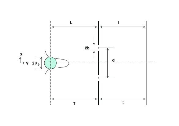
Figure 1: Sketch of a double diffraction arrangement for a two-slit grating. Parameters: $\sigma_{0}=0.5\times 10^{-5}$m, $d=10^{-7}$m, $b=1.8\times 10^{-8}$m, $L=0.1$m, $l=1.25$m, and $T=L/v$, $\tau=l/v$, where $v$ is the velocity of the molecules.

Two slit grating. We next consider the double diffraction experiment for a two slit grating following the first slit (see fig. 1). In this case the intensity at the screen is given by 7

$$I(x)=\bigl{\lvert}\Psi_{+}(x,T,\tau)+\Psi_{-}(x,T,\tau)\bigr{\rvert}^{2}\ .$$ (9)

where

$$\Psi_{\pm}(x,T,\tau) = \int_{-\infty}^{+\infty}dx_{i}\int_{-\infty}^{+\infty}dw\,K(x,T+\tau;w,T)\times$$ (10)

$$\times G(w\pm d/2)K(w,T;x_{i},0)\varphi(x_{i})$$

and

$$K(z,t;w,t_{0}) =\sqrt{\frac{m}{2\pi i\hbar(t-t_{0})}}\exp\left[i\frac{m(z-w)^{2}}{2\hbar(t-t_{0})}\right]\ ,$$ (11)

$$G(w) =\exp\left[-\frac{w^{2}}{2b^{2}}\right]\,,\ \mbox{and}$$ (12)

$$\varphi(x_{i}) =\frac{1}{\sqrt{\sigma_{0}\sqrt{\pi}}}\exp\left[-\frac{x_{i}^{2}}{2\sigma_{0}^{2}}\right].$$ (13)

The kernel $K(z,t,w,t_{0})$ is the free propagator for the particle, the functions $G(w\pm d/2)$ describe the double slit apertures which are taken to be Gaussian of width $b$ separated by a distance $d$; the width of the first slit is $\sigma_{0}$, $m$ is the mass of the particle, $T$ ($\tau$) is the time of flight from the first slit to the double slit. Parameter values are taken from ref. 8 .

Let us now allow for wave packet “ageing”, i.e., for significant transverse spreading with the accompanying $x-p$ correlation effects before reaching the two slit grating. This can be achieved in a variety of ways, but we choose for simplicity to make $\sigma_{0}$ smaller while keeping the width just before the slits fixed at $1\mu m$. The result is shown in figure 2 for different values of $\sigma_{0}$, other parameters remaining unchanged. Note the qualitative changes of the interference pattern as the $x-p$ correlations grow, implying increasing phase difference between the contributions of the impinging wave packet at the two slits with decreasing $\sigma_{0}$.

Multi-slit grating. An alternate way to bring about the effects of quantum mechanical dispersion with fixed $\sigma_{0}$ is to consider diffraction by an increasing number of equally spaced diffraction slits instead of just two. In order to explore this strategy we evaluate

$$I(x)=\lvert\sum_{n=0}^{N-1}\Psi_{n}(x,T,\tau)\rvert^{2}$$ (14)

where

$$\Psi_{n}(x,T,\tau)=\int_{-\infty}^{+\infty}dw\int_{-\infty}^{+\infty}dx_{i}K(x,T+\tau;w,T)$$

$$G(w-X_{n})K(w,T;x_{i},0)\varphi(x_{i})$$ (15)

with $X_{n}=X_{0}-(N-1)\frac{d}{2}+nd$ for $N$ slits centered around $X_{0}=0$. As discussed before, the wave function at the grating is given by

$$\Psi(x,t)\propto\exp\left[-\frac{x^{2}}{2B^{2}(t)}\Bigl{(}1-\frac{i\hbar t}{m\sigma_{0}^{2}}\Bigr{)}\right]$$ (16)

where $B(t)=\sigma_{0}\sqrt{1+(\hbar^{2}t^{2})/(m^{2}\sigma_{0}^{4})}$. Note again the second term in the exponent giving rise to the quantum dispersive phase which will be different at each slit position. An estimate of the number of slits above which the effects of the phase in equation (16) become effective (assuming an infinite transverse correlation length) is

$$N^{2}d^{2}\frac{\hbar^{2}T^{2}}{m^{2}\sigma_{0}^{4}}.$$ (17)

With the parameter values of ref. 8 and $\sigma_{0}=0.5\times 10^{-5}$m one obtains $N\sim 30$. The intensity $I(x)$ is depicted as a function of transverse position $x$ in figures 3 to 5 for different values of the number of slits $N$ (only half of the symmetric interference pattern is shown). The parameters used correspond to the experimental setup for $C_{60}$ molecules of reference 3 . In particular we take $\sigma_{0}=0.5\times 10^{-5}$m in the initial wave packet eq.(13). The grating is characterised by the half width of the slits $b$ and by the slit spacing $d$, the times $T$ and $\tau$ in eq. (Dispersion and uncertainty in multislit matter wave diffraction) are calculated from the velocity $v$ of the molecules and the distance from the first slit to the grating and from there to the detector position respectively. Each figure shows the intensity for the most probable velocity $v=200$ m/s (full line) and an incoherent sum over velocities (dotted line), which takes into account the experimental spread in the initial velocities of about $60\%$ as parameterised in reference 3 . The dash-dotted lines exhibit the corresponding classical Fraunhofer interference pattern based on the de Broglie wavelength of the $C_{60}$ molecule with $v=220$ m/s.

The classical Fraunhofer expression for the intensity is very similar to the one with a definite velocity in the first case, $N=2$. For the second case, $N=30$, deviations from the classical Fraunhofer pattern can be seen. Note also that with such a large spread in the velocities this difference will not be experimentally accessible. For larger values of $N$ as shown in figure 5 ($N=100$), the difference between a matter wave and a classical wave becomes qualitative.

These are purely quantum effects; in fact they are quantum effects coming from the first stage of the experiment and the position dependent phase. Of course these effects could be observed for a smaller number of slits provided the $x$-$p$ correlations in the first part of the experiment be large enough.

In summary, for multi-slit diffraction of matter waves we have shown that in an experiment with large enough transverse correlation length and small enough incoherence in the initial beam it is possible in principle to distinguish typical classical wave patterns from typical quantum matter wave patterns as a function of the number of slits.

Acknowledgements: The work of MCN was partially supported by CNPq, FAPESP, PRAXIS/BCC/4301/94, PRAXIS/FIS/12247/98 and POCTI/1999/FIS/3530 and MS was supported by CAPES-MEC.

.

\psfrag{p}[cc]{Position, $x\ ({\rm\mu m})$}\psfrag{i}[cc]{Intensity}\psfrag{s}[l][l][1]{$\sigma_{0}\ ({\rm\mu m})$}\psfrag{l1}[l][l][0.8]{6.0}\psfrag{l2}[l][l][0.8]{0.02}\psfrag{l3}[l][l][0.8]{0.0175}\psfrag{l4}[l][l][0.8]{0.013}\psfrag{x1}[ct][l][0.8]{-40}\psfrag{x2}[ct][l][0.8]{-20}\psfrag{x3}[ct][l][0.8]{0}\psfrag{x4}[ct][l][0.8]{20}\psfrag{x5}[ct][l][0.8]{40}\psfrag{i1}[rc][l][0.8]{0.2}\psfrag{i2}[rc][l][0.8]{0.4}\psfrag{i3}[rc][l][0.8]{0.6}\psfrag{i4}[rc][l][0.8]{0.8}\psfrag{i5}[rc][l][0.8]{1.0}\includegraphics[scale={0.6},angle={0}]{graf.eps}

Figure 2: Diffraction patterns for the arrangement of fig. 1, for different values of the width of the first slit $\sigma_{0}$. As the intensity at $x=0$ diminishes we have $\sigma_{0}=6.0\,\mu m$, $\sigma_{0}=0.02\,\mu m$, $\sigma_{0}=0.0175\,\mu m$, $\sigma_{0}=0.013\,\mu m$, respectively. Recall that the distance between two slits is $\approx 0.1\,\mu m$.

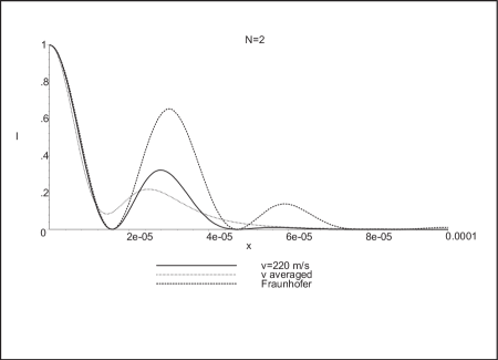
Figure 3: Intensity pattern for two slits and parameters of fig. 1.

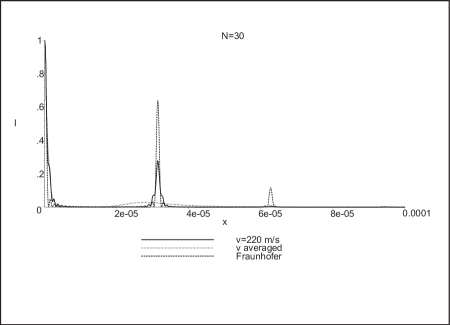
Figure 4: Intensity pattern for thirty slits and parameters of fig. 1.

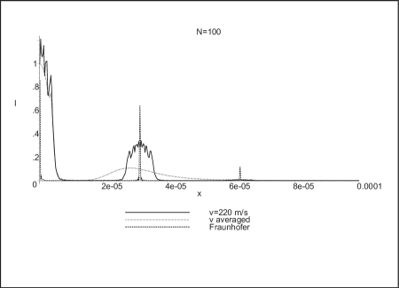
Figure 5: Intensity pattern for a hundred slits and parameters of fig. 1.

References

- (1) Davisson, C., and Germer, L., Nature 119 (1927) 558.
- (2) Gahler, R., Shull, C.G., Treimer, W., Mampe,W., and Zeilinger, A., Rev. Mod. Phys. 60 (1988) 1067.
- (3) Arndt, M., Nairz, O., Vos-Andrae, J., Kaller, C., van der Zouw, G. , and Zeilinger, A., Nature(London) 401 (1999) 680.
- (4) Nairz, O., Arndt, M., and Zeilinger, A., Am. J. Phys. 71 (2003) 319; ibid, J. Mod. Opts 47 (2000) 2811.
- (5) Gähler, R., Felber, J., Mezei, F. and Golub, R., Phys. Rev. A 58 (1998) 280.
- (6) Sinha, S. K., Tolan M. and Gibaut, A., Phys. Rev. B 57 (1998) 2740.
- (7) Viale, A., Vicari, M. and Zanghi, N., Phys. Rev. A 68 (2003) 063610.
- (8) E. Schroedinger, Proceedings of the Prussian Academy of Sciences XIX, pp. 296-303 (1930).
- (9) Nairz, O., Arndt, M., and Zeilinger, A., Phys. Rev. A 65 (2002) 032109.
.