Abstract

In this paper we consider the minimum time population transfer problem for the $z$-component of the spin of a (spin 1/2) particle driven by a magnetic field, controlled along the $x$ axis, with bounded amplitude. On the Bloch sphere (i.e. after a suitable Hopf projection), this problem can be attacked with techniques of optimal syntheses on 2-D manifolds.

Let $(-E,E)$ be the two energy levels, and $|\Omega(t)|\leq M$ the bound on the field amplitude. For each couple of values $E$ and $M$, we determine the time optimal synthesis starting from the level $-E$ and we provide the explicit expression of the time optimal trajectories steering the state one to the state two, in terms of a parameter that can be computed solving numerically a suitable equation.

For $M/E<<1$, every time optimal trajectory is bang-bang and in particular the corresponding control is periodic with frequency of the order of the resonance frequency $\omega_{R}=2E$.

On the other side, for $M/E>1$, the time optimal trajectory steering the state one to the state two is bang-bang with exactly one switching. Fixed $E$ we also prove that for $M\to\infty$ the time needed to reach the state two tends to zero. In the case $M/E>1$ there are time optimal trajectories containing a singular arc.

Finally we compare these results with some known results of Khaneja, Brockett and Glaser and with those obtained by controlling the magnetic field both on the $x$ and $y$ directions (or with one external field, but in the rotating wave approximation).

As byproduct we prove that the qualitative shape of the time optimal synthesis presents different patterns, that cyclically alternate as $M/E\to 0$, giving a partial proof of a conjecture formulated in a previous paper.

Keywords: Control of Quantum Systems, Optimal Synthesis, Minimum Time

AMS subject classifications: 49J15, 81V80

PREPRINT SISSA 82/2005/M

1 Introduction

1.1 Preliminaries

The issue of designing an efficient transfer of population between different atomic or molecular levels is crucial in atomic and molecular physics (see e.g. [8, 23, 25, 35]). In the experiments, excitation and ionization are often induced by means of a sequence of laser pulses. The transfer should be as efficient as possible in order to minimize the effects of relaxation or decoherence that are always present. In the recent past years, people started to approach the design of laser pulses by using Geometric Control Techniques (see for instance [14, 20, 21, 28, 32]). Finite dimensional closed quantum systems are in fact left (or right) invariant control systems on $SU(n)$, or on the corresponding Hilbert sphere $S^{2n-1}\subset\mathbb{C}^{n}$, where $n$ is the number of atomic or molecular levels. For these kinds of systems very powerful techniques were developed both for what concerns controllability [22, 24, 27, 33] and optimal control [4, 13, 26].

The dynamics of a $n$-level quantum system is governed by the time dependent Schrödinger equation (in a system of units such that $\hbar=1$),

$$i\dot{x}(t)=(H_{0}+\sum_{j=1}^{m}\Omega_{j}(t)H_{j})x(t){}$$ (1)

where $x(.)$, defined on $[0,T]$ is a function taking values on the state space which is $SU(n)$ (if we formulate the problem for time evolution operator) or the sphere $S^{2n-1}$ (if we formulate the problem for the wave function). The quantity $H_{0}$ called the drift Hamiltonian is an Hermitian matrix, that is natural to assume diagonalized, i.e., $H_{0}=diag(E_{1},...,E_{n})$, where $E_{1},...,E_{n}$ are real numbers representing the energy levels. With no loss of generality we can assume $\sum_{j=1}^{n}E_{j}=0$. The real valued controls $\Omega_{1}(.),...,\Omega_{m}(.)$, represent the external pulsed field, while the matrices $H_{j}$ ($j=1,...,m$) are Hermitian matrices describing the coupling between the external fields and the system. The time dependent Hamiltonian $H(t):=H_{0}+\sum_{j=1}^{m}\Omega_{j}(t)H_{j}$ is called the controlled Hamiltonian.

The first problem that usually one would like to solve is the controllability problem, i.e. proving that for every couple of points in the state space one can find controls steering the system from one point to the other. For applications, the most interesting initial and final states are of course the eigenstates of $H_{0}$.

Thanks to the fact that the control system (1) is a left invariant control system on the compact Lie group $SU(n)$, this happens if and only if

$${}\mbox{Lie}\{iH_{0},iH_{1},...iH_{m}\}=su(n),$$ (2)

(see for instance [33]). The problem of finding easily verifyable conditions under which (2) is satisfied has been deeply studied in the literature (see for instance [7]). Here we just recall that the condition (2) is generic in the space of Hermitian matrices.

Once that controllability is proved one would like to steer the system, between two fixed points in the state space, in the most efficient way. Typical costs that are interesting to minimize for applications are:

• Energy transfered by the controls to the system. $\displaystyle\int_{0}^{T}\sum_{j=1}^{m}\Omega_{j}^{2}(t)~{}dt,$

• Time of transfer. In this case one can attack two different problems one with bounded and one with unbounded controls.

The problem of minimizing time with unbounded controls is now well understood [2, 28]. On the other side, the problems of minimizing energy, or time with bounded controls are hopeless in general. Indeed optimal trajectories must satisfy a first order necessary condition for optimality called the Pontryagin Maximum Principle (in the following PMP, see for instance [4, 26]) that generalizes the Weierstraß conditions of Calculus of Variations to problems with non-holonomic constraints. For each optimal trajectory, the PMP provides a lift to the cotangent bundle that is a solution to a suitable pseudo–Hamiltonian system. Hence, the first difficulty comes from the problem of integrability of a Hamiltonian system (that generically is not integrable except for very special costs). Second, one should manage with some special solutions of the PMP, the so called abnormal and singular extremals (see for instance [9]). Finally, even if one is able to find all the solutions of the PMP (called extremal trajectories), it remains the problem of selecting, among them, the optimal trajectories, that usually is even a more difficult problem. For that purpose high order necessary conditions for optimality have been studied, like Clebsch-Legendre conditions, higher-order maximum principle, envelopes, conjugate points, index theory (cf. for instance [4, 13] and references therein). For these reasons, usually, one can hope to find a complete solution to an optimal control problem for very special costs, dynamics and in low dimension only ([5, 13, 18, 34]).

In [14, 15, 16, 17] a special class of systems, for which the analysis can be pushed much further, was studied, namely systems such that the drift term $H_{0}$ disappear in the interaction picture (by a unitary change of coordinates and a change of controls). For these systems the controlled Hamiltonian reads

$$H(t) = \left(\begin{array}[]{ccccc}E_{1}&\mu_{1}{\mathbf{\Omega}\!\!\!\!\!\Omega}_{1}(t)&0&\cdots&0\\ \mu_{1}{\mathbf{\Omega}\!\!\!\!\!\Omega}_{1}^{\ast}(t)&E_{2}&\mu_{2}{\mathbf{\Omega}\!\!\!\!\!\Omega}_{2}(t)&\ddots&\vdots\\ 0&\mu_{2}{\mathbf{\Omega}\!\!\!\!\!\Omega}_{2}^{\ast}(t)&\ddots&\ddots&0\\ \vdots&\ddots&\ddots&E_{n-1}&\mu_{n-1}{\mathbf{\Omega}\!\!\!\!\!\Omega}_{n-1}(t)\\ 0&\cdots&0&\mu_{n-1}{\mathbf{\Omega}\!\!\!\!\!\Omega}_{n-1}^{\ast}(t)&E_{n}\end{array}\right){}$$ (8)

Here $(^{\ast})$ denotes the complex conjugation involution. The controls ${\mathbf{\Omega}\!\!\!\!\!\Omega}_{1},\ldots,{\mathbf{\Omega}\!\!\!\!\!\Omega}_{n-1}$ are complex (they play the role of the real controls $\Omega_{1},\ldots,\Omega_{m}$ in (1) with $m=2(n-1)$) and $\mu_{j}>0,$ $(j=1,\ldots,n-1)$ are real constants describing the couplings (intrinsic to the quantum system) that we have restricted to couple only levels $j$ and $j+1$ by pairs.

For $n=2$ the dynamics (8) describes the evolution of the $z$ component of the spin of a (spin 1/2) particle driven by a magnetic field controlled both along the $x$ and $y$ axes, while for $n\geq 2$ it represents the first $n$ levels of the spectrum of a molecule in the rotating wave approximation (see for instance [6]), and assuming that each external fields couples only close levels. The complete solution to the optimal control problem between eigenstates of $H_{0}=diag(E_{1},\ldots,E_{n})$, has been constructed for $n=2$ and $n=3$, for the minimum time problem with bounded controls (i.e., $|{\mathbf{\Omega}\!\!\!\!\!\Omega}_{j}|\leq M_{j}$) and for the minimum energy problem $\int_{0}^{T}\sum_{j=1}^{n-1}|{\mathbf{\Omega}\!\!\!\!\!\Omega}_{j}(t)|^{2}~{}dt$ (with fixed final time).

Remark 1

For the simplest case $n=2$ (studied in [14, 21]), the minimum time problem with bounded control and the minimum energy problem actually coincide. In this case the controlled Hamiltonian is

$$H(t)=\left(\begin{array}[]{cc}-E&{\mathbf{\Omega}\!\!\!\!\!\Omega}(t)\\ {\mathbf{\Omega}\!\!\!\!\!\Omega}^{\ast}(t)&E\end{array}\right),~{}~{}~{}|{\mathbf{\Omega}\!\!\!\!\!\Omega}|\leq M,$$ (11)

and the optimal trajectories, steering the system from the first to the second eigenstate of $H_{0}=diag(-E,E)$, correspond to controls in resonance with the energy gap $2E$, and with maximal amplitude i.e. ${\mathbf{\Omega}\!\!\!\!\!\Omega}(t)=Me^{i[(2E)t+\phi]}$, where $\phi\in[0,2\pi[$ is an arbitrary phase. The quantity $\omega_{R}=2E$ is called the resonance frequency. In this case, the time of transfer $T_{\mathbb{C}}$ is proportional to the inverse of the laser amplitude. More precisely (see for instance [14]), $T_{\mathbb{C}}=\pi/(2M).$

For $n=3$ the problem has been studied in [15, 17] and it is much more complicated (in particular when the coupling constants $\mu_{1}$ and $\mu_{2}$ are different). In the case of minimum time with bounded controls, it requires some nontrivial technical tools of 2-D syntheses theory for distributional systems, that have been developed in [17].

For $n\geq 4$ the problem is hopeless, but in [16] it has been proved that the optimal controls steering the system from any couple of eigenstates of $H_{0}$ are in resonance, i.e. they oscillate with a frequency equal to the difference of energy between the levels that the control is coupling. More precisely

$${\mathbf{\Omega}\!\!\!\!\!\Omega}_{j}=A_{j}(t)e^{i[(E_{j+1}-E_{j})t+\phi_{j}]},~{}~{}~{}~{}{j=1,...,n-1}$$ (12)

where $A_{j}(.)$ are real functions describing the amplitude of the external fields and $\phi_{j}$ are arbitrary phases. Actually, this result holds for more general systems, initial and final conditions, and costs (see [16]).

The problem of minimizing time with bounded controls or energy is even more difficult if it is not possible to eliminate the drift $H_{0}$. This happens, for instance, for a system in the form (8) with real controls ${\mathbf{\Omega}\!\!\!\!\!\Omega}_{j}(t)={\mathbf{\Omega}\!\!\!\!\!\Omega}_{j}^{\ast}(t)$, $j=1,...,n-1$, as we are going to discuss now. (For more details on the elimination of the drift see [14, 15, 16].)

1.2 A spin 1/2 particle in a magnetic field

In this paper we attack the simplest quantum mechanical model interesting for applications for which it is not possible to eliminate the drift, namely a two-level quantum system driven by a real control. This system describes the evolution of the $z$ component of the spin of a (spin 1/2) particle driven by a magnetic field controlled along the $x$ axis. Equivalently it describes the first $2$ levels of a molecule driven by an external field without the rotating wave approximation. The dynamics is governed by the time dependent Schrödinger equation (in a system of units such that $\hbar=1$):

$$i\frac{d\psi(t)}{dt}=H(t)\psi(t),{}$$ (13)

where $\psi(.)=(\psi_{1}(.),\psi_{2}(.))^{T}:[0,T]\to{{\mathbb{C}}}^{2}$, $\sum_{j=1}^{2}|\psi_{j}(t)|^{2}=1$ (i.e. $\psi(t)$ belongs to the sphere $S^{3}\subset{{\mathbb{C}}}^{2}$), and

$$H(t)=\left(\begin{array}[]{cc}-E&\Omega(t)\\ \Omega(t)&E\end{array}\right),{}$$ (16)

where $E>0$ and the control $\Omega(.)$, is assumed to be a real function. With the notation of formula (1), the drift Hamiltonian is $H_{0}={\footnotesize\left(\begin{array}[]{cc}-E&0\\ 0&E\end{array}\right)}$, while $H_{1}={\footnotesize\left(\begin{array}[]{cc}0&1\\ 1&0\end{array}\right)}$, and the controllability condition (2) is satisfied.

Notice that for a spin 1/2 system, it is equivalent to treat the problem for the wave function or for the time evolution operator since $S^{3}$ is diffeomorphic to $SU(2)$. The aim is to induce a transition from the first eigenstate of $H_{0}$ (i.e., $|\psi_{1}|^{2}=1$) to any other physical state. We recall that two states $\psi,\psi^{\prime}\in S^{3}$ are physically equivalent if they differ for a factor of phase. More precisely by physical state we mean a point of the two dimensional sphere (called the Bloch sphere) $\mbox{{\bf S}}_{B}:=S^{3}/\sim$ where the equivalence relation $\sim$ is defined as follows: $\psi\sim\psi^{\prime}$ (where $\psi,\psi^{\prime}\in S^{3}$) if and only if $\psi=\exp{(i\Phi)}\psi^{\prime}$, for some $\Phi\in[0,2\pi[$. The projection from $S^{3}$ to $\mbox{{\bf S}}_{B}$ is called Hopf projection and it is given explicitly in the next section. A particularly interesting transition is of course from the first to the second eigenstates of $H_{0}$ (i.e., from $|\psi_{1}|^{2}=1$ to $|\psi_{2}|^{2}=1$).

Due to the presence of the drift, in this case the minimum time problem with bounded control and the minimum energy problem are different. In [21] the authors studied the minimum energy problem (in that case, optimal solutions can be expressed in terms of Elliptic functions), while here we minimize the time of transfer, with bounded field amplitude:

$$|\Omega(t)|\leq M,~{}~{}~{}\mbox{for every $t\in[0,T]$},$$ (17)

where $T$ is the time of the transition and $M>0$ represents the maximum amplitude available. This problem requires completely different techniques with respect to those used in [21].

Thanks to the reduction to a two dimensional problem (on the Bloch sphere), this problem can be attacked with the techniques of optimal syntheses on 2-D manifolds developed by Sussmann, Bressan, Piccoli and the first author, see for instance [11, 18, 30, 36] and recently rewritten in [13]. We make a brief recall of these techniques in Appendix A.

1.3 The Control problem on the Bloch Sphere $\mbox{{\bf S}}_{B}$

An explicit Hopf projection from $S^{3}$ to $\mbox{{\bf S}}_{B}$ is given by:

$$\Pi:\left(\begin{array}[]{ccc}{\psi_{1}}\\ {\psi_{2}}\\ {\psi_{3}}\end{array}\right)\in S^{3}\subset\mathbb{C}^{2}\longmapsto y=\left(\begin{array}[]{ccc}{y_{1}}\\ {y_{2}}\\ {y_{3}}\end{array}\right)=\left(\begin{array}[]{c}-2\,{\rm Re}(\psi_{1}^{*}\psi_{2})\\ 2\,{\rm Im}(\psi_{1}^{*}\psi_{2})\\ |\psi_{1}|^{2}-|\psi_{2}|^{2}\end{array}\right)\in\mbox{{\bf S}}_{B}\subset\mathbb{R}^{3}.$$ (27)

Notice that $\Pi$ maps the first eigenstate of $H_{0}$ (i.e. $|\psi_{1}|^{2}=1$) to the north pole $P_{N}:=(0,0,1)^{T}$ of $\mbox{{\bf S}}_{B}$, and the second eigenstate (i.e. $|\psi_{2}|^{2}=1$) to the south pole $P_{S}:=(0,0,-1)^{T}$.

After setting $u(t)=\Omega(t)/M$, the Schrödinger equation  (13), (16) projects to the following single input affine system (clarified below, after normalizations),

$$\dot{y} = F_{S}(y)+uG_{S}(y),~{}~{}|u|\leq 1,\mbox{ ~{}~{}where:}{}$$ (37)

$$y\in\mbox{{\bf S}}_{B}:=\{(y_{1},y_{2},y_{3})\in\mathbb{R}^{3},~{}~{}~{}\sum_{j=1}^{3}y_{j}^{2}=1\}$$

$$F_{S}(y):=k\cos(\alpha)\left(\begin{array}[]{c}-y_{2}\\ y_{1}\\ 0\end{array}\right),~{}~{}~{}~{}~{}G_{S}(y):=k\sin(\alpha)\left(\begin{array}[]{c}0\\ -y_{3}\\ y_{2}\end{array}\right),$$

$$\alpha:=\arctan\left(\frac{M}{E}\right)\in\,]0,\pi/2[,~{}~{}~{}k:=2E/\cos(\alpha)=2\sqrt{M^{2}+E^{2}}.{}$$

Remark 2

(normalizations) In the following, to simplify the notations, we normalize $k=1$. This normalization corresponds to a reparametrization of the time. More precisely, if $T$ is the minimum time to steer the state $\tilde{y}$ to the state $\bar{y}$ for the system with $k=1$, the corresponding minimum time for the original system is $T/(2\sqrt{M^{2}+E^{2}})$. Sometimes we need also the original system (13), (16) on $S^{3}$, with the normalization made in this remark, i.e. the system

$$i\frac{d\psi(t)}{dt}=\tilde{H}(t)\psi(t)\,,\quad\mbox{where}\quad\tilde{H}(t)=\frac{1}{2}\sin\alpha\left(\begin{array}[]{cc}-\cot\alpha&u(t)\\ u(t)&\cot\alpha\end{array}\right).$$ (40)

We come back to the original value of $k$ only in Section 3.3, where we compare our results with those of other authors.

We refer to Figure 1. The vector fields $F_{S}(y)$ and $G_{S}(y)$ (that play the role respectively of $H_{0}$ and $H_{1}$) describe rotations respectively around the axes $y_{3}$ and $y_{1}$. Let us define the vector fields corresponding to constant control $\pm 1$,

$$X^{\pm}_{S}(y):=F_{S}(y)\pm G_{S}(y).$$ (41)

The parameter $\alpha\in]0,\pi/2[$ (that is the only parameter of the problem) is the angle between the axes of rotations of $F_{S}$ and $X^{+}_{S}$. The case $\alpha\geq\pi/4$ (resp. $\alpha<\pi/4$) corresponds to $M\geq E$ (resp. $M<E$).

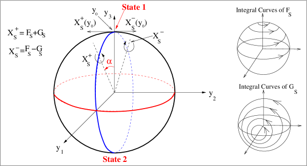
Figure 1: The Bloch Sphere

Definition 1

An admissible control $u(.)$ for the system (37)–(37) is a measurable function $u(.):[a,b]\to[-1,1]$, while an admissible trajectory is a Lipschitz functions $y(.):[a,b]\to\mbox{{\bf S}}_{B}$ satisfying (37) a.e. for some admissible control $u(.)$. If $y(.)$ is an admissible trajectory and $u(.)$ the corresponding control, we say that $(y(.),u(.))$ is an admissible pair.

For every $\bar{y}\in\mbox{{\bf S}}_{B}$, our minimization problem is then to find the admissible pair steering the north pole to $\bar{y}$ in minimum time. More precisely

Problem (P) Consider the control system (37)-(37). For every $\bar{y}\in\mbox{{\bf S}}_{B}$, find an admissible pair $(y(.),u(.))$ defined on $[0,T]$ such that $y(0)=P_{N}$, $y(T)=\bar{y}$ and $y(.)$ is time optimal.

In Optimal Control the problem (P) is known as the problem of computing the time optimal synthesis for the system (37)–(37). For more elaborated definitions of optimal synthesis see Appendix A, or [13, 31] and references therein.

Definition 2

(bang, singular for the problem (37)-(37)) A control $u(.):[a,b]\to[-1,1]$ is said to be a bang control if $u(t)=+1$ a.e. in $[a,b]$ or $u(t)=-1$ a.e. in $[a,b]$. A control $u(.):[a,b]\to[-1,1]$ is said to be a singular control if $u(t)=0$, a.e. in $[a,b]$. A finite concatenation of bang controls is called a bang-bang control. A switching time of $u(.)$ is a time $\bar{t}\in[a,b]$ such that, for every $\varepsilon>0$, $u$ is not bang or singular on $(\bar{t}-\varepsilon,\bar{t}+\varepsilon)\cap[a,b]$. A trajectory of the control system (62) is said a bang trajectory (or arc), singular trajectory (or arc), bang-bang trajectory, if it corresponds respectively to a bang control, singular control, bang-bang control. If $\bar{t}$ is a switching time, the corresponding point on the trajectory $y(\bar{t})$ is called a switching point.

Remark 3

The definitions of singular trajectory and control, given above are very specific to our problem (37)-(37). For the definition of singular trajectories for more general systems see Definition 8, Appendix A.1.

In [12] it was proved that, for the same problem (37)-(37), but in which $y\in\mathbb{R}P^{2}$, for every couple of points there exists a time optimal trajectory joining them. Moreover it was proved that every time optimal trajectory is a finite concatenation of bang and singular trajectories. Repeating exactly the same arguments and recalling that $S^{2}$ is a double covering of $\mathbb{R}P^{2}$, one easily gets the same result on $\mbox{{\bf S}}_{B}$. More precisely we have:

Proposition 1

For the problem (37)-(37), for each pair of points $p$ and $q$ belonging to $\mbox{{\bf S}}_{B}$, there exists a time optimal trajectory joining $p$ to $q$. Moreover every time optimal trajectory for the problem (37)-(37) is a finite concatenation of bang and singular trajectories.

Thus, the Fuller phenomenon (i.e. existence of an optimal trajectory joining two points with an infinite number of switchings in finite time) never occurs. Notice that the previous proposition does not apply if $\alpha=0$ or $\alpha=\pi/2$, since in these cases the controllability property is lost.

1.4 Purpose of the paper

Our aim is to study problem (P) for every possible value of the parameter $\alpha$, giving a particular relief to the case in which $\bar{y}=P_{S}$ (i.e. to the optimal trajectory steering the north to the south pole).

We will not be able to give a complete solution to the problem (P), without the help of numerical simulations. However, thanks to the theory developed in [13] we give a satisfactory description of the optimal synthesis. In the following we describe the main results and the structure of the paper.

For $\alpha<\pi/4$, every time optimal trajectory is bang-bang and in particular the corresponding control is periodic, in the sense that for every fixed optimal trajectory the time between two consecutive switchings is constant. Moreover it tends to $\pi$ as $\alpha$ goes to $0$. For the original non normalized problem this means that for $M/E<<1$, the optimal control oscillates with frequency of the order of the resonance frequency $\omega_{R}=2E$. In this case it is possible to give a satisfactory description of the optimal synthesis excluding a neighborhood of the south pole, in which we are able to compute the optimal synthesis only numerically (such results were already present in [12] as we see below).

On the other side, if $\alpha\geq\pi/4$ the computation of the optimal synthesis is simpler since the number of switchings needed to cover the whole sphere is small (less or equal than 2). In this case, for $\alpha$ big enough, we are also able to give the exact value of the time needed to cover the whole sphere. However, there is a new difficulty, namely the presence of singular arcs. Moreover the qualitative shape of the synthesis is rather different if $\alpha$ is close to $\pi/4$ or to $\pi/2$. A relevant fact is that this synthesis contains a singularity (the so called $(S,K)_{3}$) that is predicted by the general theory (see [13], pag. 61 and 82), and was never observed out from ad hoc examples.

The problem of finding explicitly the optimal trajectories from the north pole $P_{N}$ to the south pole $P_{S}$, can be easily solved in the case $\alpha\geq\pi/4$ as a consequence of the construction of the time optimal synthesis. (Coming back to the original non normalized problem we also prove that fixed $E$, for $M\to\infty$ the time of transfer from $P_{N}$ to $P_{S}$ tends to zero.)

For $\alpha<\pi/4$ the problem is more complicated. However, using the symmetries of the problem, we are able to restrict the set $\Xi$ of candidate optimal trajectories reaching the south pole, to a set containing at most 8 trajectories (half starting with control $+1$ and half starting with control $-1$, and switching exactly at the same times). These trajectories are determined in terms of a parameter (the first switching time) that can be easily computed numerically solving suitable equations. Once these trajectories are identified one can check by hands which are the optimal ones.

The analysis can be pushed much forward. We also prove that the cardinality of $\Xi$ depends on the so called normalized remainder

$$\mbox{{\tt{R}}}:=\frac{\pi}{2\alpha}-\left[\frac{\pi}{2\alpha}\right]\in[0,1[,{}$$ (42)

where $[~{}.~{}]$ denotes the integer part. In particular, for $\alpha$ small, we prove that if R is close to zero then $\Xi$ contains exactly $8$ trajectories (and in particular there are four optimal trajectories), while if R is close to $1$ then $\Xi$ contains only $4$ trajectories (two of them are optimal). The precise description of these facts is contained in Proposition 6. As a consequence, the qualitative shape of the time optimal synthesis presents different patterns, that cyclically alternate, in the non controllability limit $\alpha\to 0$, giving a partial proof of a conjecture formulated in a previous paper ([12]), that was supported by numerical simulations, see Remark 11. This is probably the most interesting byproduct of this paper.

Finally we compare these results with some known results of Khaneja, Brockett and Glaser and with those obtained by controlling the magnetic field both on the $x$ and $y$ directions.

The structure of the paper is as follows. In Section 2 we briefly resume the results of paper [12] which are connected to our problem and the conjectures formulated therein. The main results of the paper are described in Section 3, while the proofs are postponed to Appendix B. In Appendix A we recall the main tools of the theory of optimal synthesis. In Appendix C we determine the last point reached by trajectories starting at $P_{N}$ and the time needed to cover the whole sphere.

2 History of the problem and known facts

The problem (P) (although with different purposes) was already partially studied in [12], in the case $\alpha<\pi/4$. In that paper the aim was to give an estimate on the maximum number of switching for time optimal trajectories on $SO(3)$ (problem first studied by Agrachev and Gamkrelidze in [3], using index theory).

In [12] it has been proved that, for the problem (P) in the case $\alpha<\pi/4$, every optimal trajectory is bang-bang. More precisely, it was proved that in the case $\alpha<\pi/4$, if $y(.)$ is a time optimal trajectory starting at the north pole, then it should satisfy the following properties:

i)

$y(.)$ is bang bang;

ii)

the duration $s_{i}$ of the first bang arc satisfies $s_{i}\in[0,\pi]$,

iii)

the time duration between two consecutive switchings is the same for all interior bang arcs (i.e. excluding the first and the last bang) and it is the following function of $s_{i}$ defined in the interval $[0,\pi]$,

$$v(s_{i})=\pi+2\arctan\left(\frac{\sin(s_{i})}{\cos(s_{i})+\cot^{2}(\alpha)}\right).{}$$ (43)

One can immediately check that this function satisfies $v(0)=v(\pi)=\pi$ and $v(s_{i})>\pi$ for every $s_{i}\in]0,\pi[$,

iiii)

the time duration of the last arc is $s_{f}\in[0,v(s_{i})]$,

Properties i)–iiii) are illustrated in Figure 2. Moreover, thanks to the analysis given in [12], one easily get (always in the case $\alpha<\pi/4$):

v)

the number of switchings $N_{y}$ of $y(.)$ satisfies the following inequality

$$N_{y}\leq N_{M}:=\left[\frac{\pi}{2\alpha}\right]+1{}$$ (44)

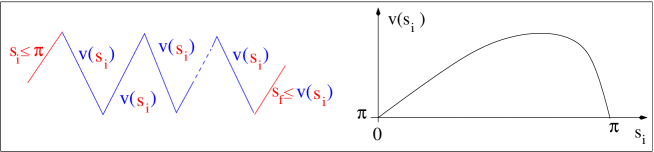
Figure 2: Time optimal trajectories for $\alpha<\pi/4$

Conditions i)-v) define a set of candidate optimal trajectories. The way in which these candidate optimal trajectories cover the whole sphere is shown in the top of Figure 3.

Consider the following curves, made by points where the control switches from $+1$ to $-1$ or viceversa, called switching curves, defined by induction

$$C_{1}^{\varepsilon}(s)=e^{X^{\varepsilon}_{S}v(s)}e^{X^{-\varepsilon}_{S}s}P_{N},\ \ \ C^{\varepsilon}_{k}(s)=e^{X^{\varepsilon}_{S}v(s)}C^{-\varepsilon}_{k-1}(s),\mbox{ (where $\varepsilon=\pm 1$ and $k=2,....,N_{M}-1$).}$$ (45)

See the top of Figure 3.

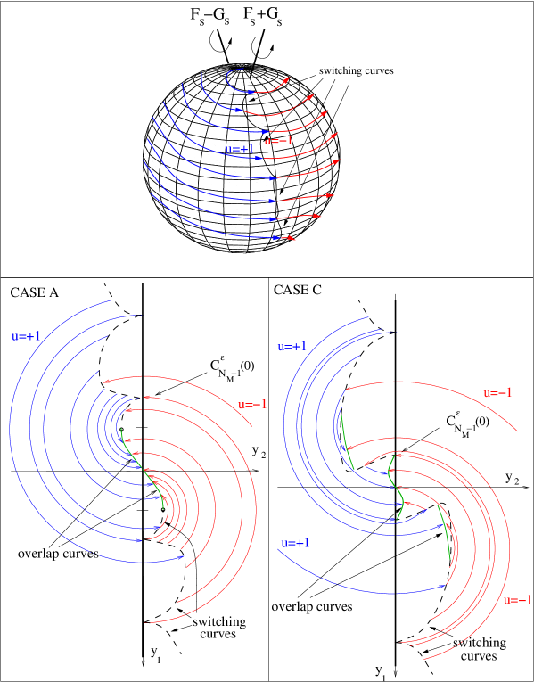
Figure 3: Synthesis on the sphere for $\alpha<\pi/4$ and conjectured shape in a neighborhood of the south pole

Even if the analysis made in [12] was sufficient to the purpose of giving a bound on the maximum number of switchings for time optimal trajectories on $SO(3)$, some questions remained unsolved. In particular questions about local optimality of the switching curves. Roughly speaking we say that a switching curve is locally optimal if it never “reflects” the trajectories (see Figure 4 A). When a family of trajectories is reflected by a switching curve then local optimality is lost and some cut locus appear in the optimal synthesis.

Definition 3

A cut locus for the problem (P) is a set of points reached at the same time by two (or more) optimal trajectories. A subset of a cut locus that is a connected ${\cal C}^{1}$ manifold is called overlap curve.

An example showing how a “reflection” on a switching curves generate a cut locus is portrayed in Figure 4 B and C. More details are given later. In [12], the following questions remain unsolved:

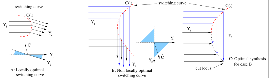
Figure 4: Locally optimal switching curves and non locally optimal switching curves with the corresponding synthesis

Question 1

Are the switching curves $C^{\varepsilon}_{k}$, $k=1...,N_{M}-1$, locally optimal? More precisely, one would like to understand how the candidate optimal trajectories described above are going to lose optimality.

Question 2

What is the shape of the optimal synthesis in a neighborhood of the south pole?

Numerical simulations suggested some conjectures regarding the above questions. More precisely:

C1

Define $k_{last}=\left[\frac{\pi-\alpha}{2\alpha}\right]-1$. Then the curves $C^{\varepsilon}_{k}(s)$, ($k=1,...,N_{M}-1$) are locally optimal if and only if $k\leq k_{last}$. Notice that $k_{last}\in\{N_{M}-3,N_{M}-2\}$.

Analyzing the evolution of the minimum time wave front in a neighborhood of the south-pole, it is reasonable to conjecture that:

C2

The shape of the optimal synthesis in a neighborhood of the south pole depends on the so called remainder $r:=\pi-2\alpha\left[\frac{\pi}{2\alpha}\right].$ Notice that $r$ belongs to the interval $[0,2\alpha[$. More precisely, we conjecture that for $\alpha\in]0,\pi/4[$, there exist two positive numbers $\alpha_{1}$ and $\alpha_{2}$ such that $0<\alpha_{1}<\alpha<\alpha_{2}<2\alpha$ and:

CASE A: $r\in]\alpha_{2},2\alpha[$. The switching curve $C^{\varepsilon}_{N_{M}-1}$ glues to an overlap curve that passes through the origin (Fig. 3, Case  A).

CASE B: $r\in[\alpha_{1},\alpha_{2}]$. The switching curve $C^{\varepsilon}_{N_{M}-1}$ is not reached by optimal trajectories in the interval $]0,\pi]$. At the point $C^{\varepsilon}_{N_{M}-1}(0)$ an overlap curve starts and passes through the origin.

CASE C: $r\in]0,\alpha_{1}[$. The situation is more complicated and it is depicted in the bottom of Fig. 3, Case C.

For $r=0$, the situation is the same as in CASE A, but for the switching curve starting at $C^{\varepsilon}_{N_{M}-2}(0)$.

3 Main Results

We give here a brief description of the main results of the paper. The corresponding proofs are given in Appendix B. From now on we use the following conventions.

Remark 4

(notation) The letter $B$ refers to a bang trajectory and the letter $S$ refers to a singular trajectory. A concatenation of bang and singular trajectories is labeled by the corresponding letter sequence, written in order from left to right. Sometimes, we use a subscript to indicate the time duration of a trajectory so that we use $B_{t}$ to refer to a bang trajectory defined on an interval of length $t$ and, similarly, $S_{t}$ for a singular trajectory defined on an interval of length $t$. Moreover we indicate by $\gamma^{+}$ (resp. $\gamma^{-}$) the trajectory of (37)–(37) starting at the north pole at time zero and corresponding to control $u\equiv 1$ (resp. $u\equiv-1$). Notice that $\gamma^{\pm}$ are defined for every time, and are periodic. Finally we use the following subsets of $\mbox{{\bf S}}_{B}$: the circle of equation $y_{3}=0$ called equator, the set $y_{3}>0$, called north hemisphere and the set $y_{3}<0$, called south hemisphere.

3.1 Optimal synthesis for $\alpha\geq\pi/4$

In this section we describe the time optimal synthesis for $\alpha\geq\pi/4$. We divide $\mbox{{\bf S}}_{B}$ in 8 open regions called $\Omega^{\pm}_{1},...,\Omega^{\pm}_{3}$, $\Omega_{\mbox{\footnotesize nasty}}^{\pm}$ and in 16 arcs (see Definition 4, and Figure 5). For every point $\bar{y}\in\mbox{{\bf S}}_{B}\setminus(\Omega_{\mbox{\footnotesize nasty}}^{+}\cup\Omega_{\mbox{\footnotesize nasty}}^{-})$, Theorem 1 gives the optimal trajectories reaching $\bar{y}$.

Unlike the $\alpha<\pi/4$ case, here it is possible to detect the presence of singular trajectories that are optimal, and also of cut loci (even not only in a neighborhood of the south pole).

The region $\Omega_{\mbox{\footnotesize nasty}}^{+}$ (and similarly $\Omega_{\mbox{\footnotesize nasty}}^{-}$) is more difficult to analyze. It contains a cut locus that should be determined numerically. Even if we are not able to provide an analytic characterization of this locus, we are able to prove the following.

i)

$\alpha=\arcsin(1/\sqrt[4]{2})$ is a bifurcation point for the optimal synthesis i.e. the qualitative shape is different if $\alpha\in[\pi/4,\arcsin(1/\sqrt[4]{2})[$ (called Case 1) or $\alpha\in[\arcsin(1/\sqrt[4]{2}),\pi/2[$ (called Case 2). More precisely, from the point $D^{+}:=\gamma^{+}(\pi)$, in Case 1 it starts an optimal switching curve, while in Case 2 it starts an overlap curve (see Proposition 3). The situation in $\Omega_{\mbox{\footnotesize nasty}}^{-}$ is symmetric.

ii)

The south pole belongs to the cut locus and it is reached exactly by four optimal trajectories (see Proposition 2).

Numerical computations show that in Case 2, the cut locus in $\Omega_{\mbox{\footnotesize nasty}}^{+}$ is an overlap curve connecting $D^{+}$ with the south pole, while in Case 1, the switching curve starting from $D^{+}$ loses local optimality at a point of $\Omega_{\mbox{\footnotesize nasty}}^{+}$ and connects to an overlap curve which reaches the south pole (see Figure 6). Remark 9 explains that in Case 2 it is not necessary to compute the cut locus lying in $\Omega_{\mbox{\footnotesize nasty}}^{+}$ to get the expression of the optimal trajectory connecting $P_{N}$ to a point of $\Omega_{\mbox{\footnotesize nasty}}^{+}$. The situation in $\Omega_{\mbox{\footnotesize nasty}}^{-}$ is symmetric.

Let us start with the description of the optimal synthesis in $\mbox{{\bf S}}_{B}\setminus(\Omega_{\mbox{\footnotesize nasty}}^{+}\cup\Omega_{\mbox{\footnotesize nasty}}^{-})$. Even if Definition 4 and Theorem 1 look complicated, the shape of the optimal synthesis is quite simple as it is shown in Figure 6.

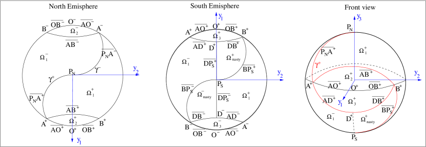
Figure 5: Definition 4

Definition 4

According to Figure 5, let us define the following curves on $\mbox{{\bf S}}_{B}$.

• Let $t_{1}$ be the first time at which $\gamma^{+}$ intersects the equator and let $A^{+}:=\gamma^{+}(t_{1})$ (notice that $t_{1}=\pi-\arccos(\cot^{2}(\alpha))$). Define $\overline{P_{N}A^{+}}=Supp\left(\gamma^{+}|_{[0,t_{1}]}\right)$.

• Let $\xi^{-}$ be the trajectory corresponding to control $-1$, starting at time zero from $A^{+}$. Let $t_{2}$ be the first positive time at which $\xi^{-}$ intersects the equator (notice that $t_{2}=2\arccos(\cot^{2}(\alpha))$). Define $B^{+}:=\xi^{-}(t_{2})$ and $\overline{AB^{+}}=Supp\left(\xi^{-}|_{[0,t_{2}]}\right)$.

• Let $O^{+}=(1,0,0)$. Define $\overline{AO^{+}}$ (resp. $\overline{OB^{+}}$) as the support of the trajectory corresponding to control zero, starting at $A^{+}$ (resp. $O^{+}$) and ending at $O^{+}$ (resp. $B^{+}$).

• Recall that $D^{+}=\gamma^{+}(\pi)$, and define $\overline{AD^{+}}=Supp\left(\gamma^{+}|_{[t_{1},\pi]}\right)$, $\overline{DB^{+}}=Supp\left(\gamma^{+}|_{[\pi,t_{3}]}\right)$, where $t_{3}$ is the second intersection time of $\gamma^{+}$ with the equator (notice that $t_{3}=\pi+\arccos(\cot^{2}(\alpha))=t_{1}+t_{2}$).

• Let $\overline{BP_{S}^{+}}$ the support of the trajectory corresponding to control $-1$, starting at $B^{+}$ and ending at the south pole.

• Let $\overline{DP_{S}^{+}}$ the connected subset of the meridian $y_{2}=0$, lying in the south hemisphere and connecting the point $D^{+}$ to the south pole.

Similarly define $A^{-},$ $B^{-},$ $O^{-}$, $D^{-}$, $\overline{P_{N}A^{-}}$, $\overline{AB^{-}}$, $\overline{AO^{-}}$, $\overline{OB^{-}}$, $\overline{AD^{-}}$, $\overline{DB^{-}}$, $\overline{BP_{S}^{-}}$, $\overline{DP_{S}^{-}}$ .

According to Figure 5 define $\Omega_{1}^{\pm},\ldots,\Omega_{4}^{\pm},\Omega_{\mbox{\footnotesize nasty}}^{\pm}$ as the open connected components of the open set obtained subtracting from $\mbox{{\bf S}}_{B}$ all the arcs defined above.

The following theorem holds for every $\alpha\in]\pi/4,\pi/2[$. For the particular value $\alpha=\pi/4$ the claims of the theorem must be modified. Such changes are reported in Remark 5.

Theorem 1

Let $\gamma\!\!\!\gamma$${}_{\bar{y}}$ be the set of time optimal trajectories steering the north pole to $\bar{y}$. We have the following:

T1.

If $\bar{y}\in\overline{P_{N}A^{+}}$ then $\gamma\!\!\!\gamma$${}_{\bar{y}}$ is made by a unique trajectory corresponding to control $+1$ of the form $B_{t}$, with $t\leq t_{1}$.

T2.

If $\bar{y}\in\overline{AB^{+}}\setminus B^{+}$ then $\gamma\!\!\!\gamma$${}_{\bar{y}}$ is made by a unique trajectory of the form $B_{t_{1}}B_{t}$ (with the first bang corresponding to control $+1$).

T3.

If $\bar{y}\in\overline{AO^{+}}$ then $\gamma\!\!\!\gamma$${}_{\bar{y}}$ is made by a unique trajectory of the form $B_{t_{1}}S_{s}$ (with the first bang corresponding to control $+1$).

T4.

If $\bar{y}\in\overline{OB^{+}}\setminus O^{+}$ then $\gamma\!\!\!\gamma$${}_{\bar{y}}$ is made by two trajectories of the form $B_{t_{1}}S_{s}B_{t}$, both starting with control $+1$ and ending respectively with control $+1$ and $-1$. These two trajectories have the same values of $s\geq 0$ and $t>0$.

T5.

If $\bar{y}\in\overline{AD^{+}}$ then $\gamma\!\!\!\gamma$${}_{\bar{y}}$ is made by a unique trajectory corresponding to control $+1$ of the form $B_{t}$, with $t\in[t_{1},\pi]$.

T6.

If $\bar{y}\in\overline{DB^{+}}\setminus B^{+}$ then $\gamma\!\!\!\gamma$${}_{\bar{y}}$ is made by a unique trajectory corresponding to control $+1$ of the form $B_{t}$, with $t\in[\pi,t_{3}[$.

T7.

If $\bar{y}\in\overline{BP_{S}^{+}}$ then $\gamma\!\!\!\gamma$${}_{\bar{y}}$ is made by two trajectories respectively of the form $B_{t_{1}}B_{t}$ and $B_{t_{3}}B_{t-t_{2}}$ and starting with control $+1$.

T8.

If $\bar{y}\in\Omega_{1}^{+}\cup(\overline{DP_{S}^{-}}\setminus P_{S})$, then $\gamma\!\!\!\gamma$${}_{\bar{y}}$ is made by a unique trajectory of the form $B_{t}B_{t^{\prime}}$, with $0\leq t<t_{1}$ and the first bang corresponding to control $+1$.

T9.

If $\bar{y}\in\Omega_{2}^{+}$, then $\gamma\!\!\!\gamma$${}_{\bar{y}}$ is made by a unique trajectory of the form $B_{t_{1}}S_{s}B_{t}$, with $s>0$, the first bang arc and the last bang arc corresponding respectively to control $+1$ and $-1$.

T10.

If $\bar{y}\in\Omega_{3}^{+}$, then $\gamma\!\!\!\gamma$${}_{\bar{y}}$ is made by a unique trajectory of the form $B_{t_{1}}S_{s}B_{t}$, with $s>0$ and both bang arcs corresponding to control $+1$.

T11.

If $\bar{y}=P_{S}$ then $\gamma\!\!\!\gamma$${}_{\bar{y}}$ is made by the four trajectories of the form $B_{t_{1}}B_{t_{3}}$ and $B_{t_{3}}B_{t_{1}}$.

T12.

If $\bar{y}\in\Omega_{\mbox{\footnotesize nasty}}^{+}$ then every trajectory of $\gamma\!\!\!\gamma$${}_{\bar{y}}$ is bang-bang with at most two switchings.

If $\bar{y}$ belongs to one of the remaining sets defined above, the description of the optimal strategy is analogous, by symmetry.

Remark 5

In the case $\alpha=\pi/4$ some changes in the previous statement are required. In particular the points $A^{+}$,$B^{+}$,$O^{+}$ and $D^{+}$ coincide (also the points $A^{-}$,$B^{-}$,$O^{-}$ and $D^{-}$ coincide) and, consequently, there are no optimal trajectories containing singular arcs. Another immediate consequence of this fact is that there are only two optimal trajectories reaching the south pole, of the form $B_{\pi}B_{\pi}$.

Remark 6

Notice that every point of $\overline{OB^{+}}\setminus O^{+}$, $\overline{OB^{-}}\setminus O^{-}$, $\overline{BP_{S}^{+}}$, $\overline{BP_{S}^{-}}$ is reached by more than one optimal trajectory, i.e. it belongs to the cut locus. Other points of the cut locus can be identified numerically in $\Omega_{\mbox{\footnotesize nasty}}^{+}$ and $\Omega_{\mbox{\footnotesize nasty}}^{-}$ as explained in the next section.

Remark 7

In Theorem 1 we do not specify all the durations of the bang arcs. However the missing ones can be obtained simply by following the switching strategy backwards.

Remark 8

Note that the region reached by optimal trajectories containing a singular arc $\Omega_{2}^{\pm}\cup\Omega_{3}^{\pm}\cup\overline{AO^{\pm}}\cup\overline{OB^{\pm}}$ become bigger and bigger as $\alpha$ tends to $\pi/2$. Moreover, in this limit, since the modulus of the drift $F_{S}$ becomes smaller and smaller, the time needed to cover such region tends to infinity. Notice however that the time needed to reach $P_{S}$ is always $2\pi$. The time needed to reach every point of the sphere for $\alpha$ big enough, and the last point reached by an optimal trajectory containing a singular arc, can be computed explicitly. This is done in Appendix C.

Since the case $\bar{y}=P_{S}$ is important also for the determination of the cut locus in $\Omega_{\mbox{\footnotesize nasty}}^{+}\cup\Omega_{\mbox{\footnotesize nasty}}^{-}$, it is reported in the next section as a separate proposition (see Proposition 2).

Figure 6: Optimal synthesis for $\alpha=\pi/3$ and $\alpha$ slightly larger than $\pi/4$.

.

3.1.1 The time optimal synthesis in $\Omega_{\mbox{\footnotesize nasty}}^{\pm}$ and optimal trajectories reaching $P_{S}$ for $\alpha\geq\pi/4$

From next proposition, T11 of Theorem 1 follows. More precisely Proposition 2 shows that in the case $\alpha\geq\pi/4$, there are exactly four optimal trajectories steering $P_{N}$ to $P_{S}$, and it characterizes them. As a consequence, the south pole belongs to the cut locus.

Proposition 2

Consider the control system (37)–(37), and assume $\alpha\geq\pi/4$. Then the optimal trajectories steering the north pole to the south pole are bang-bang with only one switching. More precisely they are the four trajectories corresponding to the four controls

$$u^{(1)}=\left\{\begin{array}[]{l}u=1,~{}t\in[0,t_{1}]\\ u=-1,~{}t\in]t_{1},T],\\ \end{array}\right.~{}u^{(2)}=\left\{\begin{array}[]{l}1,~{}t\in[0,t_{3}]\\ -1,~{}t\in]t_{3},T],\\ \end{array}\right.~{}u^{(3)}=\left\{\begin{array}[]{l}-1,~{}t\in[0,t_{1}]\\ 1,~{}t\in]t_{1},T],\\ \end{array}\right.~{}u^{(4)}=\left\{\begin{array}[]{l}-1,~{}t\in[0,t_{3}]\\ 1,~{}t\in]t_{3},T]\\ \end{array}\right.$$ (54)

where $t_{1}$ and $t_{3}$ are defined in Definition 4, and $T=2\pi.$

One can easily check that the switchings described in Proposition 2 occur on the equator ($y_{3}=0$).

The following proposition describes the optimal synthesis in $\Omega_{\mbox{\footnotesize nasty}}^{\pm}$, in a neighborhood of the points $D^{\pm}$ and the bifurcation occurring at $\alpha=\arcsin(1/\sqrt[4]{2})$.

Proposition 3

Let $\alpha\geq\pi/4$. In a neighborhood of the point $D^{+}$ in $\Omega_{\mbox{\footnotesize nasty}}^{+}$, there exists a switching curve starting at $D^{+}$ of the form $e^{v(s)X_{S}^{+}}e^{sX_{S}^{-}}P_{N}$. If $\alpha>\pi/4$ this curve is tangent to the equator at $D^{+}$. Moreover if $\alpha<\arcsin(1/\sqrt[4]{2})$ (above called Case 1) then the switching curve is optimal near $D^{+}$, while if $\alpha\geq\arcsin(1/\sqrt[4]{2})$ (above called Case 2) then the switching curve is not locally optimal near $D^{+}$ and an overlap curve starts at the point $D^{+}$. A symmetric result holds in a neighborhood of $D^{-}$ in $\Omega_{\mbox{\footnotesize nasty}}^{-}$.

The region $\Omega_{\mbox{\footnotesize nasty}}^{+}$ contains a cut locus that should be determined numerically. In Case 2, numerical simulations show that the switching curve starting at $D^{+}$ is never optimal, i.e. every point of $\Omega_{\mbox{\footnotesize nasty}}^{+}$ is reached by an optimal trajectory of the form $e^{tX_{+}}e^{sX_{-}}P_{N}$, with $s\in]0,t_{1}[$ or an optimal trajectory of the form $e^{tX_{-}}e^{sX_{+}}P_{N}$, with $s\in]\pi,t_{3}[$.

Remark 9

Notice however that, in Case 2, given a point $\bar{y}\in\Omega_{\mbox{\footnotesize nasty}}^{+}$, to find the time optimal trajectory reaching $\bar{y}$, it is not necessary to compute the cut locus. Indeed it is sufficient to compare the final times, corresponding to the two switching strategies given above, and to chose the quickest one. The situation in $\Omega_{\mbox{\footnotesize nasty}}^{-}$ is symmetric.

In Case 1, the situation is more complicated. The switching curve described by Proposition 3 has the expression $C_{1}^{+}(s)=e^{X^{+}_{S}v(s)}e^{X^{-}_{S}s}P_{N}$, $s\in]0,t_{1}[$ where the function $v(.)$ is given by the same formula of the $\alpha<\pi/4$ case, i.e. $v(s)=\pi+2\arctan\left[{(\sin s)}/({\cos s+\cot^{2}\alpha})\right].$ (To verify such formula it is enough to repeat the computations done in [12].) As described by Proposition 3, this switching curve is optimal near $D^{+}$ and numerical simulations show that there exists $\bar{s}\in]0,t_{1}[$ such that there is an optimal trajectory switching on $C_{1}^{+}(s)$ if and only if $s\in[0,\bar{s}[$, and an overlap curve connecting $C_{1}^{+}(\bar{s})$ to the south pole appears. The optimal synthesis for Case 1 and Case 2 is depicted in Figure 6.

3.2 Optimal trajectories reaching the south pole for $\alpha<\pi/4$

In this section we characterize the time optimal trajectories reaching the south pole, in the case $\alpha<\pi/4$. This characterization is more complicated with respect to the case $\alpha\geq\pi/4$, due to the fact that the optimal trajectories have many switchings. The time optimal synthesis for $\alpha<\pi/4$ was already (partially) studied in [12] and it has been described in Section 2.

From conditions i)–iiii) in Section 2, we know that every optimal trajectory starting at the north pole has the form $B_{s_{i}}{B_{v({s_{i}})}\cdots B_{v({s_{i}})}}B_{s_{f}}$ where the function $v(s_{i})$ is given by formula (43). (In the following we do not specify if the first bang corresponds to control $+1$ or $-1$, since, as a consequence of the symmetries of the problem, if $u(t)$ is an optimal control steering the north pole to the south pole, $-u(t)$ steers the north pole to the south pole as well.) It remains to identify one or more values of $s_{i},s_{f}$ and the corresponding number of switchings $n$ for this trajectory to reach the south pole.

Notice that $\bar{t}=\arccos(-\tan^{2}(\alpha))$ is the maximum of the function $v(.)$ on the interval $[0,\pi]$, $v(.)$ is increasing on $[0,\bar{t}]$ and decreasing on $[\bar{t},\pi]$ and $v(0)=v(\pi)=\pi$. Then, given $s\in[0,\pi]$ such that $s\neq\bar{t}$, there is a unique solution $s^{\ast}(s)\in[0,\pi]$, $s^{\ast}(s)\neq s$, to the equation $v(s^{\ast})=v(s)$. The function $s^{\ast}(.)$ is extended to the whole interval $[0,\pi]$ setting $s^{\ast}(\bar{t})=\bar{t}$ (see Figure 7 A). Thanks to the symmetries of the problem, we prove that if $\alpha<\pi/4$, $s_{f}$ is equal either to $s_{i}$ or to $s^{\ast}(s_{i})$. This fact is described by Lemma 4 stated and proved in Appendix B.

Figure 7: Graph of $v(.)$ when $\alpha=\pi/6$ (figure A). Graph of the functions $\mathcal{F}$ and $\mathcal{G}$ when $\alpha=0.13$ (figure B and C)

The following two propositions describe how to identify candidate triples $(s_{i},s_{f},n)$ for which the corresponding trajectory steers the north pole to the south pole in minimum time. We say that a bang-bang trajectory, solution of the system (37)–(37), is a candidate optimal trajectory if it is an extremal trajectory for problem (P) reaching the south pole and it has a number $n$ of switchings satisfying $n\leq N_{M}$ (defined in Formula (44)). From Lemma 4, there are two kinds of candidate optimal trajectories:

• $s_{f}=s^{\ast}(s_{i})$, called TYPE-1-candidate optimal trajectories

• $s_{f}=s_{i}$ called TYPE-2-candidate optimal trajectories

Define the following functions, whose geometric meaning is clarified in Appendix B.2:

$$\theta(s)\!=\!2\arccos\!\left(\sin^{2}\!\left(\frac{v(s)}{2}\right)\cos(2\alpha)-\cos^{2}\!\left(\frac{v(s)}{2}\right)\right)\!\!{}$$ (55)

$$\beta(s)=2\arccos(\sin(\alpha)\cos(\alpha)(1-\cos(s))){}$$ (56)

Proposition 4

(TYPE-1-trajectories) Fixed $\alpha<\pi/4$, the equation for the couple $(s,n)\in[0,\pi]\times\mathbb{N}$:

$$\mathcal{F}(s):=\frac{2\pi}{\theta(s)}=n,{}$$ (57)

has either two or zero solutions. More precisely if $(s,n)$ is a solution to equation (57), then $(s^{\ast}(s),n)$ is the second one. The trajectories $B_{s}\underbrace{B_{v({s})}\cdots B_{v({s})}}_{n-1}B_{s^{\ast}(s)}$ and $B_{s^{\ast}(s)}\underbrace{B_{v({s})}\cdots B_{v({s})}}_{n-1}B_{s}$ are the TYPE-1-candidate optimal trajectories.

Proposition 5

(TYPE-2-trajectories) Fixed $\alpha<\pi/4$, the equation for the couple $(s,n)\in[0,\pi]\times\mathbb{N}$:

$$\mathcal{G}(s):=\frac{2\beta(s)}{\theta(s)}+1=n,{}$$ (58)

has exactly two solutions. More precisely these solutions have the form $(s_{1},n)$, $(s_{2},n+1)$. The trajectories $B_{s_{1}}\underbrace{B_{v({s_{1}})}\cdots B_{v({s_{1}})}}_{n-1}B_{s_{1}}$ and $B_{s_{2}}\underbrace{B_{v({s_{2}})}\cdots B_{v({s_{2}})}}_{n}B_{s_{2}}$ are the TYPE-2-candidate optimal trajectories.

In Figure 7 B and C the graphs of the functions (57) and (58) are drawn for a particular value of $\alpha$, namely $\alpha=0.13$. Propositions 4 and 5 select a set of (possibly coinciding) $4$ or $8$ candidate optimal trajectories (half of them starting with control $+1$ and the other half with control $-1$) corresponding to triples $(s_{i},s_{f},n)$. Such triples can be easily computed numerically solving equations (57) and (58). Then the optimal trajectories can be selected by comparing the times needed to reach the south pole for each of the candidate optimal trajectory. Notice that there are at least two optimal trajectories steering the north to the south pole (one starting with control $+1$ and the other with control $-1$).

If $\pi/(2\alpha)$ is an integer number $\bar{n}$, then TYPE-1 candidate optimal trajectories coincide with the TYPE-2 candidate optimal trajectories of the form $B_{\pi}\underbrace{B_{\pi}...B_{\pi}}_{\bar{n}-2}B_{\pi}$. The remaining trajectories of TYPE-2 are of the form $B_{s}\underbrace{B_{v(s)}...B_{v(s)}}_{\bar{n}-1}B_{s}$ for some $s\in]0,\pi[$. Otherwise if $\pi/(2\alpha)$ is not an integer number, define:

$$m:=[\frac{\pi}{2\alpha}],~{}~{}~{}\mbox{and the normalized remainder}~{}~{}~{}\mbox{{\tt{R}}}:=\frac{\pi}{2\alpha}-\left[\frac{\pi}{2\alpha}\right]\in[0,1[.$$

where $[.]$ denotes the integer part. The following proposition determines precisely the time optimal trajectories for particular values of the parameter R:

Proposition 6

For $m$ large enough there exist $r_{1}(m)\leq r_{2}(m)\in]0,1[$ such that:

A.

if $\mbox{{\tt{R}}}\in]0,r_{1}(m)]$ then equation (57) admits exactly two solutions that are both optimal, while TYPE-2 candidate optimal trajectories are not.

B.

if $\mbox{{\tt{R}}}\in]r_{1}(m),r_{2}(m)[$, then equation (57) admits two solutions, that are not optimal.

C.

if $\mbox{{\tt{R}}}\in]r_{2}(m),1[$ then equation (57) does not admit any solution. Moreover $r_{2}(m)\to 0$ for $m\to\infty$.

Remark 10

The function $r_{2}(m)$ can be determined explicitly (see Appendix B.2.1), while for $r_{1}(m)$ we are just able to prove the existence, and we conjecture that it can be taken equal to $r_{2}(m)$.

Remark 11

An important consequence of Proposition 6 is that for $\alpha$ small, the number of optimal trajectories reaching the south pole is not fixed with respect to $\alpha$. Indeed such number alternates as $\alpha\to 0$, according to Proposition 6: in particular it is equal to $4$ if $\mbox{{\tt{R}}}\in]0,r_{1}(m)]$ and it is equal to $2$ if $\mbox{{\tt{R}}}\in]r_{2}(m),1[\cup\{0\}$. This is enough to conclude that also the qualitative shape of the optimal synthesis in a neighborhood of the south pole alternates giving a partial proof to the conjecture C2 of Section 2 (originally stated in [12]). In particular it is a proof of the first assertion (on the dependence of the synthesis on the remainder $r=2\alpha\mbox{{\tt{R}}}$). Moreover notice that the results of Proposition 6 perfectly fit with all the other statements of conjecture C2 with $r_{2}(m)$ playing the role of $\alpha_{1}/(2\alpha)$. One can apply the definition of locally equivalent syntheses given in [13] (see Definition 32, pag. 59), to make rigorous the statement that the qualitative shape of the optimal synthesis changes with $\alpha$.

Using the previous analysis one can easily show the following result (of which we skip the proof):

Proposition 7

If $N$ is the number of switchings of an optimal trajectory joining the north to the south pole, then

$$\frac{\pi}{2\alpha}-1\leq N<\frac{\pi}{2\alpha}+1.$$

Using these inequalities and the fact that, for $\alpha<\pi/6$, the function $\ \displaystyle{2s+\left(\frac{\pi}{2\alpha}-1\right)v(s)}\$ is increasing on $[0,\pi]$, one can give a rough estimate of the time needed to reach the south pole:

Proposition 8

The total time $T$ of an optimal trajectory joining the north to the south pole satisfies the inequalities:

$$\frac{\pi^{2}}{2\alpha}-2\pi<T<\frac{\pi^{2}}{2\alpha}+\pi.$$

3.3 Comparison with results in the rotating wave approximation and with [28]

In this section we come back to the original value of $k$ i.e. $k=2E/\cos(\alpha)=2\sqrt{M^{2}+E^{2}}$, and we compare the time necessary to steer the state one to the state two for our model and the model (11), described in Remark 1, in which we control the magnetic field both along the $x$ and $y$ direction, or we consider a two-level molecule in the rotating wave approximation. We recall that $-E,E$ are the energy levels and $M$ is the bound on the control. For our model, the time of transfer $T$ satisfies:

• for $\alpha\geq\pi/4$ (i.e. for $M\geq E$) then $T=2\pi/k=\pi/\sqrt{M^{2}+E^{2}}$;

• for $\alpha<\pi/4$ (i.e. for $M<E$) then $T$ is estimated by $\displaystyle\frac{1}{k}\left(\frac{\pi^{2}}{2\alpha}-2\pi\right)<T<\frac{1}{k}\left(\frac{\pi^{2}}{2\alpha}+\pi\right).$

On the other hand, for the model (11), the time of transfer is $T_{\mathbb{C}}=\pi/(2M)$ (cfr. Remark 1).

Figure 8:  A. Estimate of the minimum time to reach the state two and comparison with the time needed with two controls or in the rotating wave approximation    B. Comparison between the optimal strategy for our system and in the rotating wave approximation

Fixed $E=1$, in Figure 8 A the times $T$ and $T_{\mathbb{C}}$ as function of $M$ are compared. Notice that although $T_{\mathbb{C}}$ is bigger than the lower estimate of $T$ in some interval, we always have $T_{\mathbb{C}}\leq T$. This is due to the fact that the admissible velocities of our model are a subset of the admissible velocities of the model (11).

Notice that, fixed $E=1$, for $M\to 0$ we have $T\sim\pi^{2}/(4M)=(\pi/2)T_{\mathbb{C}}$, while for $M\to\infty$, we have $T\sim\pi/M=2T_{\mathbb{C}}$.

Remark 12

For $M<<E$ (i.e. for $\alpha$ small) the difference between two switching times is $v(s)/k\sim\pi/(2E)$. It follows that a time optimal trajectory connecting the north to the south pole (in the interval between the first and the last bang) is periodic with period $P\sim\pi/E$ i.e. with a frequency of the order of the resonance frequency $\omega_{R}=2E$ (see Figure 8 B). On the other side if $M>E$ then the time optimal trajectory connecting the north with the south pole is the concatenation of two pulses. Notice that if $M>>E$, the time of transfer is of the order of $\pi/M$ and therefore tends to zero as $M\to\infty$. It is interesting to compare this result with a result of Khaneja, Brockett and Glaser, for a two level system, but with no bound on controls (see [28]). They estimate the infimum time to reach every point of the whole group $SU(2)$ in $\pi/E$. On the other side, in Appendix C it is proved that the time needed to cover the whole sphere $\mbox{{\bf S}}_{B}=SU(2)/S^{1}$ goes to $\pi/(4E)$ as $M$ goes to infinity (however this does not contradict the fact that the state two can be reached in an arbitrary small time, as we discussed above).

Notice that our optimal control has the same form of the control computed in [28] i.e. a pulse (bang) followed by an evolution with the drift (singular) followed by a pulse (bang).

Appendix A An overview on Optimal Synthesis on 2-D Manifolds

In this section we briefly recall the theory of optimal syntheses on 2-D manifolds for system of the kind $\dot{y}=F(y)+uG(y)$, $|u|\leq 1$, developed by Sussmann, Bressan, Piccoli and the first author in [11, 18, 30, 36] and recently rewritten in [13]. This appendix is written to be as much self-consistent as possible.

For every coordinate chart on the manifold it is possible to introduce the following three functions:

$$\Delta_{A}(y) := Det(F(y),G(y))=F_{1}(y)G_{2}(y)-F_{2}(y)G_{1}(y),{}$$ (59)

$$\Delta_{B}(y) := Det(G(y),[F,G](y))=G_{1}(y)[F,G]_{2}(y)-G_{2}(y)[F,G]_{1}(y),{}$$ (60)

$$f_{S}(y) := -\Delta_{B}(y)/\Delta_{A}(y).{}$$ (61)

The sets $\Delta_{A}^{-1}(0),\Delta_{B}^{-1}(0)$ of zeroes of $\Delta_{A},\Delta_{B}$ are respectively the set of points where $F$ and $G$ are parallel, and the set of points where $G$ is parallel to $[F,G]$. These loci are fundamental in the construction of the optimal synthesis. In fact, assuming that they are smooth embedded one dimensional submanifold of $M$ we have the following:

• in each connected region of $M\setminus(\Delta_{A}^{-1}(0)\cup\Delta_{B}^{-1}(0))$, every extremal trajectory is bang-bang with at most one switching. Moreover, for every switching of the extremal trajectory the value of the control passes from $-1$ to $+1$ if $f_{S}>0$ and from $+1$ to $-1$ if $f_{S}<0$;

• the support of singular trajectories (that are trajectories for which the switching function identically vanishes, see Definition 7 below) is always contained in the set $\Delta_{B}^{-1}(0)$;

• a trajectory not switching on the set of zeroes of $G$ is an abnormal extremal (i.e. a trajectory for which the Hamiltonian given by the PMP vanishing, see below) if and only if it switches on the locus $\Delta_{A}^{-1}(0)$.

Then the synthesis is built recursively on the number of switchings of extremal trajectories, canceling at each step the non optimal trajectories (see [13], Chapter 1).

Remark 13

Notice that, although the functions $\Delta_{A}$ and $\Delta_{B}$ depend on the coordinate chart, the sets $\Delta_{A}^{-1}(0)$, $\Delta_{B}^{-1}(0)$ and the function $f_{S}$ do not, i.e. they are intrinsic objects of the control equation $\dot{y}=F(y)+uG(y)$.

A.1 Basic Definitions and PMP on a $n$-dimensional Manifold

In this section we define our optimization problem, we state the Pontryagin Maximum Principle, and we give some basic definitions in the more general case of a $n$-dimensional manifold. We do this, since in Appendix B.1 we stated some result for the original problem (40), on $S^{3}\sim SU(2)$.

Problem (Q) Consider the control system:

$$\dot{y}=F(y)+uG(y),~{}~{}~{}y\in M,~{}~{}~{}|u|\leq 1,{}$$ (62)

where:

(H0)

$M$ is a smooth $n$-dimensional manifold. The vector fields $F(y)$ and $G(y)$ are ${\cal C}^{\infty}$.

We are interested in the problem of reaching every point of $M$ in minimum time from a point $y_{0}\in M$.

Definition 5

An admissible control $u(.)$ for the system (62) is a measurable function $u(.):[a,b]\to[-1,1]$, while an admissible trajectory is a Lipschitz functions $y(.):[a,b]\to M$ satisfying $\dot{y}(t)=F(y(t))+u(t)G(y(t))$ a.e. for some admissible control $u(.)$

In the following we assume that the control system is complete i.e. for every measurable control function $u(.):[a,b]\to[-1,1]$ and every initial state $\bar{y}$, there exists a trajectory $y(.)$ corresponding to $u(.)$, which is defined on the whole interval $[a,b]$ and satisfies $y(a)=\bar{y}$. For us a solution to the problem (Q) is an optimal synthesis. For a more elaborated definition of synthesis, see Section A.3.

Definition 6

(Optimal Synthesis) An optimal synthesis for the problem (Q) is a collection of time optimal trajectories $\Gamma=\{y_{y_{1}}(.):[0,b_{y_{1}}]\mapsto M$, $y_{1}\in M:~{}~{}y_{y_{1}}(0)=y_{0},~{}y_{y_{1}}(b_{y_{1}})=y_{1}\}$.

The key tool is the PMP (see [4, 13, 26]).

Theorem (Pontryagin Maximum Principle for the problem (Q)) Consider the control system (62) subject to (H0). Define for every $(y,\lambda,u)\in T^{\ast}M\times[-1,1]$ the function

$$\mathscr{H}(y,\lambda,u) := <\lambda,F(y)>+u<\lambda,G(y)>.$$

If the couple $(y(.),u(.)):[0,T]\to M\times[-1,1]$ is time optimal then there exist a never vanishing Lipschitz continuous covector $\lambda(.):t\in[0,T]\mapsto\lambda(t)\in T^{\ast}_{y(t)}M$ and a constant $\lambda_{0}\leq 0$ such that for a.e. $t\in[0,T]$:

i)

$\dot{y}(t)=\displaystyle{\frac{\partial\mathscr{H}}{\partial\lambda}(y(t),\lambda(t),u(t))}$,

ii)

$\dot{\lambda}(t)=-\displaystyle{\frac{\partial\mathscr{H}}{\partial y}(y(t),\lambda(t),u(t))=-\lambda(t)\big{(}\nabla F(y(t))+u(t)\nabla G(y(t))\big{)}}$,

iii)

$\mathscr{H}(y(t),\lambda(t),u(t))=\mathscr{H}_{M}(y(t),\lambda(t))$ where $\mathscr{H}_{M}(y,\lambda):=\max\{\mathscr{H}(y,\lambda,u):u\in[-1,1]\},$

iiii)

$\mathscr{H}_{M}(y(t),\lambda(t))+\lambda_{0}=0$.

Remark 14

The PMP is just a necessary condition for optimality. A trajectory $y(.)$ (resp. a couple $(y(.),\lambda(.))$) satisfying the conditions given by the PMP is said to be an extremal (resp. an extremal pair). An extremal corresponding to $\lambda_{0}=0$ is said to be an abnormal extremal, otherwise we call it a normal extremal.

We are now interested in determining the extremal trajectories satisfying the conditions given by the PMP. A key role is played by the following:

Definition 7

(switching function) Let $(y(.),\lambda(.))$ be an extremal pair. The corresponding switching function is defined as $\phi(t):=<\lambda(t),G(y(t))>$.

Notice that $\phi(.)$ is continuously differentiable (indeed $\dot{\phi}(t)=<\lambda(t),[F,G](y(t))>$, that is continuous).

Definition 8

(bang, singular) Let $\gamma$, defined in $[a,b]$, be an extremal trajectory and $u(.):[a,b]\to[-1,1]$ the corresponding control. We say that $u(.)$ is a bang control if $u(t)=+1$ a.e. in $[a,b]$ or $u(t)=-1$ a.e. in $[a,b]$. We say that $u(.)$ is singular if the corresponding switching function $\phi(t)=0$ in $[a,b]$. A finite concatenation of bang controls is called a bang-bang control. A switching time of $u(.)$ is a time $\bar{t}\in[a,b]$ such that, for every $\varepsilon>0$, $u$ is not bang or singular on $(\bar{t}-\varepsilon,\bar{t}+\varepsilon)\cap[a,b]$. An extremal trajectory of the control system (62) is said a bang extremal, singular extremal, bang-bang extremal respectively, if it corresponds to a bang control, singular control, bang-bang control respectively. If $\bar{t}$ is a switching time, the corresponding point on the trajectory $y(\bar{t})$ is called a switching point.

The switching function is important because it determines where the controls may switch. In fact, using the PMP, one easily gets:

Proposition 9

A necessary condition for a time $t$ to be a switching is that $\phi(t)=0$. Therefore, on any interval where $\phi$ has no zeroes (respectively finitely many zeroes), the corresponding control is bang (respectively bang-bang). In particular, $\phi>0$ (resp $\phi<0$) on $[a,b]$ implies $u=1$ (resp. $u=-1$) a.e. on $[a,b]$. On the other hand, if $\phi$ has a zero at $t$ and $\dot{\phi}(t)$ is different from zero, then $t$ is an isolated switching.

A.2 More on singular extremals and predicting switchings for 2-D systems

Now we come back to the case in which $M$ is two dimensional. In this Section we compute the control corresponding to singular extremals and we would like to predict which kind of switchings can happen, using properties of the vector fields $F$ and $G$. The following two lemmas illustrate the role of the functions $\Delta_{A}^{-1}(0)$, $\Delta_{B}^{-1}(0)$ in relation with singular and abnormal extremals. The proofs can be found in [11, 13, 30].

Lemma 1

Let $y(.)$ be an extremal trajectory that is singular in $[a,b]\subset Dom(y(.))$. Then $y(.)|_{[a,b]}$ corresponds to the so called singular control $\varphi(y(t))$, where:

$${}\varphi(y)=-\frac{\nabla\Delta_{B}(y)\cdot F(y)}{\nabla\Delta_{B}(y)\cdot G(y)},$$ (63)

with $\Delta_{A}$ and $\Delta_{B}$ defined in Eqs. (59) and (60). Moreover, on $Supp(y(.))$, $\varphi(y)$ is always well-defined and its absolute value is less than or equal to one. Finally $Supp(y(.)|_{[a,b]})\subset\Delta_{B}^{-1}(0)$.

Lemma 2

Let $y(.)$ be a bang-bang extremal for the control problem (62), $t_{0}\in Dom(y(.))$ be a time such that $\phi(t_{0})=0$ and $G(y(t_{0}))\neq 0$. Then, the following conditions are equivalent: i) $y(.)$ is an abnormal extremal; ii) $y(t_{0})\in\Delta_{A}^{-1}(0)$; iii) $y(t)\in\Delta_{A}^{-1}(0)$, for every time $t\in Dom(y(.))$ such that $\phi(t)=0$.

The following lemma describes what happens when $\Delta_{A}$ and $\Delta_{B}$ are different from zero.

Lemma 3

Let $\Omega\subset M$ be an open set such that $\Omega\cap(\Delta_{A}^{-1}(0)\cup\Delta_{B}^{-1}(0))=\emptyset$. Then all connected components of $Supp(y(.))\cap\Omega$, where $y(.)$ is an extremal trajectory of (62), are bang-bang with at most one switching. Moreover, if $f_{S}>0$ throughout $\Omega$, then $y(.)|_{\Omega}$ is associated to a constant control equal to $+1$ or $-1$ or has a switching from $-1$ to $+1$. If $f_{S}<0$ throughout $\Omega$, then $y(.)|_{\Omega}$ is associated to a constant control equal to $+1$ or $-1$ or has a switching from $+1$ to $-1$.

A.3 Frame Curves and Frame Points

For the problem (Q), under generic conditions on the vector fields $F$ and $G$, one can make the complete classification of synthesis singularities, stable synthesis, singularities of the minimum time wave fronts.

In the following, for sake of completeness, we recall the main results on existence of an optimal synthesis and on classification of synthesis singularities obtained in [29, 30] (see also [13]). In [29], it was proved that the control system (62), under generic conditions on $F$ and $G$ (with the additional assumption $F(y_{0})=0$) admits a time optimal regular synthesis in finite time $T$, starting from $y_{0}$. By generic conditions, we mean conditions verified on an open and dense subset of the set of ${\cal C}^{\infty}$ vector fields endowed with the ${\cal C}^{3}$ topology (see [13], formula 2.6 pp. 39). To define what we mean by regular synthesis, we first need to introduce the concept of reachable set and of stratification of the reachable set. We call reachable set in time $T>0$, the set:

$${\cal R}(T) := \{y\in M:\ \exists~{}b_{y}\in[0,T]\mbox{ and a trajectory }$$

$$\gamma_{y}:[0,b_{y}]\to M\mbox{ of (\ref{sys-gen}) such that }\gamma_{y}(0)=y_{0},~{}\gamma_{y}(b_{y})=y\}.$$

Then we need the definition of stratification of ${\cal R}(T)$, that roughly speaking is a partition in manifolds of different dimensions.

Definition 9

(stratification) A stratification of ${\cal R}(T)$, $T>0$, is a finite collection $\{M_{i}\}$ of connected embedded ${\cal C}^{1}$ submanifolds of $M$, called strata, such that ${\cal R}(T)=\cup_{k}M_{k}$, and the following holds. If $M_{j}\cap Clos(M_{k})\not=\emptyset$ with $j\not=k$ then $M_{j}\subset Clos(M_{k})$ and $dim(M_{j})<dim(M_{k})$.

Then a time optimal regular synthesis is defined by: i) a family of time optimal trajectories $\Gamma=\{\gamma_{y}:[0,b_{y}]\to M$, $y\in{\cal R}(T):~{}~{}\gamma_{y}(0)=y_{0},~{}\gamma_{y}(b_{y})=y\}$ such that if $\gamma_{y}\in\Gamma$ and $\bar{y}=\gamma_{y(t)}$ for some $t\in[0,b_{y}]$, then $\gamma_{\bar{y}}=\gamma_{y}|_{[0,t]}$; ii) a stratification of ${\cal R}(T)$ such that the optimal trajectories of $\Gamma$ can be obtained from a feedback $u(y)$ satisfying:

• on strata of dimension 2, $u(y)=\pm 1$,

• on strata of dimension 1, called frame curves (FC for short), $u(y)=\pm 1$ or $u(y)=\varphi(y)$, where $\varphi(y)$ is defined by (63).

The strata of dimension 0 are called frame points (FP). Every FP is an intersection of two FCs. In [30] (see also [13]), it is provided a complete classification of all types of FPs and FCs, under generic conditions. All the possible FCs are:

• FCs of kind $Y$ (resp. $X$), corresponding to subsets of the trajectories $\gamma^{+}$ (resp. $\gamma^{-}$) defined as the trajectory starting at $y_{0}$ with constant control $+1$ (resp. constant control $-1$);

• FCs of kind $C$, called switching curves, i.e. curves made of switching points;

• FCs of kind $S$, i.e. singular extremals;

• FCs of kind $K$, called overlaps and reached optimally by two trajectories coming from different directions;

• FCs which are arcs of optimal trajectories starting at FPs. These trajectories “transport” special information.

The FCs of kind $Y,C,S,K$ are depicted in Fig. 9. There are eighteen topological equivalence classes of FPs. A detailed description can be found in [10, 13, 30].

Figure 9: Frame Curves of the optimal synthesis, under generic conditions

Appendix B Proof of the Main Results

In this section we give the proof of our main results. We start with a lemma, stating a property of optimal trajectories, that is a consequence of the symmetries of the problem. It is used to identify the time optimal trajectories steering the north to the south pole both for $\alpha\geq\pi/4$ and $\alpha<\pi/4$.

Lemma 4

Let $\alpha\in]0,\pi/2[$. Every optimal bang-bang trajectory, connecting the north to the south pole, with more than one switching is such that $v(s_{i})=v(s_{f})$ where $s_{i}$ is the first switching time, $s_{f}$ is the time needed to steer the last switching point to the south pole and $v(s_{i})$ is the time between two consecutive switchings.

Proof of Lemma 4. Consider the problem of connecting $P_{S}$ with $P_{N}$ in minimum time for the system $\dot{z}=F^{\prime}_{S}(z)+uG^{\prime}_{S}(z)$ where $z\in S^{2}$ and $F^{\prime}_{S}(z)=-F_{S}(z)$, $G^{\prime}_{S}(z)=-G_{S}(z)$. The trajectories of this system coincide with those of the system (37)–(37), but the velocity is reversed. Therefore the optimal trajectories for the new problem coincide with the optimal ones for the system (37)–(37) connecting $P_{N}$ to $P_{S}$, and the time between two switchings is the same. Since performing the change of coordinates $(z_{1},z_{2},z_{3})\rightarrow(y_{1},y_{2},y_{3})=(-z_{1},z_{2},-z_{3})$, the new problem becomes exactly the original problem, we deduce that, if we have more than one switching, it must be $v(s_{i})=v(s_{f})$.  

B.1 Time Optimal Synthesis for the two Level Quantum System for $\alpha\geq\pi/4$

In this section, we apply the theory of optimal syntheses on 2-D manifolds recalled in Appendix A, to the system (37)–(37). Our aim is to describe the time optimal synthesis for $\alpha\geq\pi/4$, i.e. to prove Theorem 1 and Propositions 2 and 3. First we state some general results, holding for $\alpha\in]0,\pi/2$[, regarding time optimal trajectories of the system (40), on $S^{3}\sim SU(2)$, analogous to those obtained in [12] for $SO(3)$ (in particular the proofs can be repeated using the same arguments).

B.1.1 General results on $S^{3}$

In this section $\alpha\in]0,\pi/2$[. The first proposition states that singular extremals, defined as extremals for which the switching function vanishes (see Definitions 7 and 8) correspond to zero control. This fact is very specific for our problem.

Proposition 10

For the normalized minimum time problem on $S^{3}$ (40), singular extremals are integral curves of the drift, i.e. they must correspond to a control almost everywhere vanishing.

Since for a fixed $u\in[-1,1]$ every trajectory of (40) is periodic with period $\frac{4\textstyle{\pi}}{\sqrt{u^{2}\sin^{2}\alpha+\cos^{2}\alpha}}$ we have that:

Proposition 11

Given an extremal trajectory $\gamma$ of type $B_{t}$ (resp $S_{t}$), then $t<4\pi$ (resp. $t<\frac{4\pi}{\cos\alpha}$).

The following proposition describes the switching behavior of abnormal and bang-bang normal extremals (see Section A.1 for the definition).

Proposition 12

Let $\gamma$ be an abnormal extremal of (40). Then it is bang-bang and the time duration between two consecutive switchings is always equal to $\pi$. In other words, $\gamma$ is of kind $B_{s}B_{\pi}...B_{\pi}B_{t}$ with $s,t\leq\pi$.
On the other hand, if $\gamma$ is a bang-bang normal extremal, then the time duration ${\cal T}$ along an interior bang arc is the same for all interior bang arcs and verifies $\pi<{\cal T}<2\pi$ (i.e. $\gamma$ is of kind $B_{s}B_{{\cal T}}...B_{{\cal T}}B_{t}$ with $s,t\leq{\cal T}$).

For the optimal trajectories containing a singular arc we have the following:

Proposition 13

Let $\gamma$ be a time optimal trajectory containing a singular arc. Then $\gamma$ is of the type $B_{t}S_{s}B_{t^{\prime}}$, with $s\leq\frac{2\pi}{\cos\alpha}$ if $t>0$ or $t^{\prime}>0$ and $s<\frac{4\pi}{\cos\alpha}$ otherwise.

These results on $S^{3}\sim SU(2)$ are useful to determine the optimal synthesis on $\mbox{{\bf S}}_{B}$, since every optimal trajectory on $\mbox{{\bf S}}_{B}$ is the projection of an optimal trajectory on $S^{3}$. This is a simple consequence of the fact that $\mbox{{\bf S}}_{B}$ is an homogeneous space of $SU(2)$:

Proposition 14

A time optimal trajectory $\gamma$ for the system (37)–(37) on $\mbox{{\bf S}}_{B}$ starting at $P_{N}$ is the projection of a time optimal trajectory of (40) starting from a point satisfying $|\psi_{1}|^{2}=1$ (recall that $\psi=(\psi_{1},\psi_{2})^{T}\in S^{3}\subset\mathbb{C}^{2}$).

Remark 15

Notice that, since two opposite points on $S^{3}$ project on the same point on $\mbox{{\bf S}}_{B}$, it is easy to see from Proposition 11, that the projection on $\mbox{{\bf S}}_{B}$ of an optimal trajectory of (40) of type $B_{t}$ (resp $S_{t}$), must be such that $t<2\pi$ (resp. $t<\frac{2\pi}{\cos\alpha}$). More precisely, for a fixed $u\in[-1,1]$ every trajectory of (37)–(37) is periodic with period $\frac{2\textstyle{\pi}}{\sqrt{u^{2}\sin^{2}\alpha+\cos^{2}\alpha}}$ (the period divides by two after projection).

B.1.2 Construction of the Synthesis on $\mbox{{\bf S}}_{B}$

In this section we assume $\alpha\geq\pi/4$. Following Appendix A we first need to determine the sets $\Delta_{A}^{-1}(0)$, $\Delta_{B}^{-1}(0)$, and the function $f_{S}$. Checking where $F_{S}$ is parallel to $G_{S}$ and where $G_{S}$ is parallel to $[F_{S},G_{S}]$, one gets $\Delta_{A}^{-1}(0)=\{y\in\mbox{{\bf S}}_{B}:y_{2}=0\}$ and $\Delta_{B}^{-1}(0)=\{y\in\mbox{{\bf S}}_{B}:y_{3}=0\}$. To find the function $f_{S}$ we can choose for instance the coordinate chart defined on each hemisphere by the projection on the plain $\{(y_{1},y_{2})\in\mathbb{R}^{2}\}$, obtaining $f_{S}=(\sin\alpha)y_{3}/y_{2}$. Then Lemma 3 says that, every optimal trajectory belonging to one of the regions $\{y\in\mbox{{\bf S}}_{B}:y_{3}>0,y_{2}>0\}$, $\{y\in\mbox{{\bf S}}_{B}:y_{3}<0,y_{2}<0\}$ is bang-bang with at most one switching. Moreover only the switching from control $-1$ to control $+1$ is allowed. On the contrary, on the regions $\{y\in\mbox{{\bf S}}_{B}:y_{3}>0,y_{2}<0\}$, $\{y\in\mbox{{\bf S}}_{B}:y_{3}<0,y_{2}>0\}$, the control can switch only from $+1$ to $-1$. Moreover, thanks to Lemma 1, every singular extremal must lie on the equator. The following lemma characterizes the structure of the bang-bang extremals for the problem (P).

Lemma 5

Recall that $t_{1}=\pi-\arccos(\cot^{2}\alpha)$ and $t_{3}=\pi+\arccos(\cot^{2}\alpha)$ and consider a bang-bang extremal for the problem (P). Then it is of the form $B_{s}B_{v(s)}B_{v(s)}\ldots$ with $s\in[0,t_{1}]\cup[\pi,t_{3}]$, where, on the set $\,[0,t_{1}[\cup[\pi,t_{3}[\,$, $v(.)$ is defined as follows:

$$v(s):=\pi+2\arctan\left(\frac{\sin s}{\cos s+\cot^{2}\alpha}\right).$$

If $\alpha=\pi/4$ then $t_{1}=t_{3}=\pi$ and $v(\pi):=\pi$, while if $\alpha>\pi/4$ we set $v(t_{1}):=v(t_{3}):=2\pi$.

Notice that the function $v(.)$ has the same expression (43) obtained in the case $\alpha<\pi/4$ (excepted at the points $t_{1}$ and $t_{3}$). However its interval of definition is different.

Proof of Lemma 5. As shown above, the meridian $\Delta_{A}^{-1}(0)$ and the equator $\Delta_{B}^{-1}(0)$ divide the sphere in four parts and in each of them the sign of the function $f_{S}$ is constant and changes when passing through $\Delta_{A}^{-1}(0)$ or $\Delta_{B}^{-1}(0)$. In particular, following $\gamma^{+}$ or $\gamma^{-}$ (cfr Remark 4) in the case in which $\alpha>\pi/4$ this happens at the times $t_{1}$ (where the equator is crossed), at time $\pi\,$ (where $\Delta_{A}^{-1}(0)$ is crossed) and at time $\,t_{3}$ (again is the equator to be crossed). Applying Lemma 3, we obtain that for an extremal trajectory the first switching may occur only on the intervals $[0,t_{1}]\,$ and $\,[\pi,t_{3}]$. Exactly as in [12], one shows that the extremal must have the form $B_{s}B_{v(s)}B_{v(s)}\ldots$ with $s\in[0,t_{1}]\cup[\pi,t_{3}]$. The case $\alpha=\pi/4$ is similar.  

Remark 16

One can also show that every trajectory starting from $P_{N}$, of the form $B_{s}B_{v(s)}B_{v(s)}\ldots$ with $s\in[0,t_{1}]\cup[\pi,t_{3}]$ is extremal i.e., for every $s$ in such set, there exists an initial value of the covector $\lambda$ such that the switching function $\phi(.)$ vanishes for the first time at time $s$.

Unlike the case in which $\alpha<\pi/4$, in the case $\alpha>\pi/4$ it is possible to establish the presence of optimal trajectories containing a singular arc, whose switching strategy is described by the following proposition, illustrated in Figure 10 A.

Proposition 15

Let $\alpha\geq\pi/4$. A trajectory $\gamma$ of (37)–(37) starting with control $u=1$ and containing a singular arc is a solution of (P) if and only if it is of the form $B_{t}S_{s}B_{t^{\prime}}$ and satisfies the following conditions:

• $t=t_{1}=\pi-\arccos(\cot^{2}\alpha)$ i.e. $\gamma$ coincides with $\gamma^{+}$ until it reaches the equator.

• $s\leq\arccos(\cot\alpha)/\cos\alpha$ i.e. the singular arc is optimal until it reaches the point $O^{+}=(1,0,0)^{T}$.

• If $s=\arccos(\cot\alpha)/\cos\alpha$, then the trajectory is of type $B_{t}S_{s}$ (i.e. the time duration of the last bang arc reduces to zero). If $s<\arccos(\cot\alpha)/\cos\alpha$, then $\gamma$ is optimal until the last bang arc reaches the equator (i.e. it does not exist $\bar{t}\in]0,t^{\prime}[$ such that $\gamma(t+s+\bar{t})$ is contained in the equator).

An analogous result holds for trajectories starting with control $-1$.

Remark 17

Notice that in the case $\alpha=\pi/4$, Proposition 15 provides a singular trajectory degenerated to a point. In other words for $\alpha=\pi/4$ there are no singular trajectories that are optimal.

Remark 18

Notice that the previous result completely characterizes the optimal synthesis in some neighborhoods of the points $O^{\pm}=(\pm 1,0,0)^{T}$, namely $\Omega_{2}^{\pm}\cup\Omega_{3}^{\pm}$, and moreover it determines the presence of two symmetric overlap curves contained inside the equator. The synthesis around the point $O^{+}$ is represented in Figure 10 A.

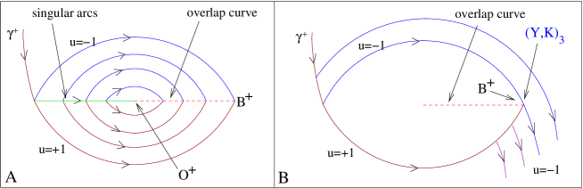
Figure 10: The region covered by optimal trajectories with singular arcs and the $(Y,K)_{3}$ frame point

Proof of Proposition 15. Consider a trajectory, that is a solution of (P) starting with $u=+1$ and containing a singular arc. Using Propositions 13 and 14 this trajectory must be of the form $B_{t}S_{s}B_{t^{\prime}}$ and, since the singular arc is contained inside the equator, we have $t=t_{1}$ (the case $t=t_{3}$ can be easily excluded). Consider a singular arc containing in its interior the point $O^{+}$. This arc contains two points of the form $(y_{1}^{0},-y_{2}^{0},0)^{T}$ and $(y_{1}^{0},y_{2}^{0},0)^{T}$, with both $y_{1}^{0}$, $y_{2}^{0}$ positive, that can be connected by a bang arc. Using classical comparison theorems for second order ODEs, one can easily compare the time needed to follow such trajectory with the time needed to steer the two points along the singular arc finding that the bang arc is quicker than the singular arc. Therefore a singular arc containing $O^{+}$ cannot be optimal. By symmetry, the extremal trajectories that have the same singular arc, but the last bang arc corresponding to opposite control, must meet on a point of the equator. Therefore the arc of the equator which is comprised between the point $O^{+}$ (resp $O^{-}$) and the second intersection point with $\gamma^{+}$ (resp. $\gamma^{-}$) is an overlap curve. It remains now to verify that the trajectories described above are optimal (until the last bang arc reaches the equator). This is a straightforward consequence of the fact that the quickest bang-bang trajectories that enter the region spanned by such trajectories (i.e. the closure of the regions $\Omega^{\pm}_{2}\cup\Omega^{\pm}_{3}$) are not extremal because of Lemma 3.  

Remark 19

Notice the trivial fact that, if a trajectory $\gamma$ defined on the interval $[a,b]$ is optimal between $\gamma(a)$ and $\gamma(b)$, then the restriction of $\gamma$ in $[c,d]$, $c,d\in[a,b]$, $c<d$, is optimal between $\gamma(c)$ and $\gamma(d)$.

Using Remark 19, we have that Proposition 15 characterizes completely the time optimal synthesis on $\overline{P_{N}A^{\pm}}$ and in the closure of $\Omega_{2}^{\pm}\cup\Omega_{3}^{\pm}$, i.e. it proves items T1–T6, T9 and T10, of Theorem 1.

Remark 20

From Lemma 5 we obtain that there are four families of bang-bang trajectories. In particular the families starting with control $+1$ and switching respectively in $[0,t_{1}]$ and $[\pi,t_{3}]$ join at the point $B^{+}$, generating an amazing $(Y,K)_{3}$ frame point, in the framework of the classification of [13]. See Figure 10 B.

Next we give the proof of Proposition 2, from which it follows T11 of Theorem 1, and, using again Remark 19, also T7.

Proof of Proposition 2 By Proposition 15, there are no optimal trajectories containing a singular arc joining $P_{N}$ with $P_{S}$. One can easily see that the only possible trajectories steering $P_{N}$ to $P_{S}$ with only one switching are those described in the statement of the proposition, that we have to compare with trajectories having more than one switching. Trajectories having two switchings with the first or the last bang longer than $\pi$ and trajectories with more than two switchings are excluded since from Lemma 5 their total time is larger than $2\pi$. Trajectories having two switchings and length of the first arc $s_{i}$ and the length of the last arc $s_{f}$ satisfying $s_{i},s_{f}<\pi$ are excluded since by Lemma 4 they must satisfy $s_{i}=s_{f}$. For these trajectories the total time can be easily computed and it is $\,2\pi+2\arcsin\left(\frac{1}{2\sin(\alpha)}\right)>2\pi$.  

Item T8 is proved by the following:

Proposition 16

If $\bar{y}\in\Omega_{1}^{+}\cup(\overline{DP_{S}^{-}}\setminus P_{S})$, then $\gamma\!\!\!\gamma$${}_{\bar{y}}$ is made by a unique trajectory of the form $B_{t}B_{t^{\prime}}$, with $0\leq t<t_{1}$ and the first bang corresponding to control $+1$. A similar result holds if $\bar{y}\in\Omega_{1}^{-}\cup(\overline{DP_{S}^{+}}\setminus P_{S})$. As a consequence there is not a cut locus in the region $\Omega_{1}^{+}\cup\Omega_{1}^{-}$. On the other hand $\Omega_{\mbox{\footnotesize nasty}}^{+}\cup\Omega_{\mbox{\footnotesize nasty}}^{-}$ contains a cut locus.

Proof of Proposition 16 Define the following three families of extremal trajectories:

$$\gamma^{A}_{s}(t) := e^{tX_{S}^{+}}e^{sX_{S}^{-}}P_{N},\mbox{~{}~{}with~{}~{}}s\in]0,t_{1}[\mbox{~{}~{}and~{}~{}}t\leq v(s),$$

$$\gamma^{B}_{s}(t) := e^{tX_{S}^{-}}e^{sX_{S}^{+}}P_{N},\mbox{~{}~{}with~{}~{}}s\in[\pi,t_{3}[\mbox{~{}~{}and~{}~{}}t\leq v(s),$$

$$\gamma^{C}_{s}(t) := e^{tX_{S}^{-}}e^{v(s)X_{S}^{+}}e^{sX_{S}^{-}}P_{N},\mbox{~{}~{}with~{}~{}}s\in]0,t_{1}[\mbox{~{}~{}and~{}~{}}t\leq v(s).$$

First notice that from Proposition 2, there are no optimal trajectories of kind $\gamma^{A}_{s}$ reaching the arc $\overline{BP_{S}^{+}}$. Now for every point $x\in\overline{DP_{S}^{+}}$ the following happens: i) there exist $s_{A},~{}t_{A}$ such that $x=\gamma^{A}_{s_{A}}(t_{A})$, and they are unique; ii) if there exist $s_{B},~{}t_{B}$ (resp. $s_{C},~{}t_{C}$) such that $x=\gamma^{B}_{s_{B}}(t_{B})$, (resp. $x=\gamma^{C}_{s_{C}}(t_{C})$), then they are unique. By direct computation, one can compare the times the three trajectories need to reach $x$, i.e. $s_{A}+t_{A},s_{B}+t_{B},s_{C}+v(s_{C})+t_{C}$, finding that the optimal trajectory is of kind $\gamma^{A}$ (these computations are long, not very instructive, and we omit them). From this fact the first part of the claim immediately follows. Moreover it implies that there is not a cut locus in $\Omega_{1}^{+}$, since the only trajectories entering such region are those of the form $\gamma^{A}$. The existence of a cut locus in $\Omega_{\mbox{\footnotesize nasty}}^{+}$ is evident, since no optimal trajectory belonging to the families $\gamma^{A}$, $\gamma^{B}$, $\gamma^{C}$ leaves $\Omega_{\mbox{\footnotesize nasty}}^{+}$. The reasoning in $\Omega_{1}^{-}$ and in $\Omega_{\mbox{\footnotesize nasty}}^{-}$ is similar.  

End of the proof of Theorem 1
To conclude the proof of Theorem 1, it remains to prove T12. Consider by contradiction an optimal bang-bang trajectory $\gamma$ defined in $[0,t_{\gamma}]$ steering $P_{N}$ to a point of $\Omega_{\mbox{\footnotesize nasty}}^{+}$, with at least three switchings. Define $\bar{t}=\max\{t\in[0,t_{\gamma}]:\gamma(t)\notin\Omega_{\mbox{\footnotesize nasty}}^{+}\}$. Then, by Remark 19, $\gamma|_{[0,\bar{t}]}$ must be optimal between $P_{N}$ and $\gamma(\bar{t})$. Then, from the results proved above, we deduce that $\gamma|_{[0,\bar{t}]}$ can have at most one switching. Therefore $\gamma$ switches at least two times in $\Omega_{\mbox{\footnotesize nasty}}^{+}$ and the arc between them must be completely contained in $\Omega_{\mbox{\footnotesize nasty}}^{+}$ and this leads to a contradiction since the sign of $f_{S}$ is constant in $\Omega_{\mbox{\footnotesize nasty}}^{+}$ (see Lemma 3).  

Before proving Proposition 3, notice that the point $D^{+}$, which is obtained following the trajectory $\gamma^{+}$ for a time $\pi$ (see Figure 6), belongs to two different families of bang-bang trajectories at time $\pi$, one given by trajectories starting with control $-1$ and switching at time $s\leq t_{1}$, the other one given by trajectories that start with control $1$ and switching at time $s\in[\pi,t_{3}]$. Moreover, since $v(0)=\pi$, there must be a switching curve starting at $D^{+}$ and therefore we deduce that there are two possible behaviors of the optimal synthesis around this point: either this switching curve is optimal or the two fronts continue to intersect generating an overlap curve.
Observe that if $\alpha\geq\pi/3$ the trajectories of the type $B_{s}B_{v(s)}B_{t}$ with $s$ small cannot be optimal since the vector fields $X^{+}_{S}$ and $X^{-}_{S}$ point to opposite sides on the switching curve (i.e. the switching curve “reflects the trajectories”, see footnote 1). In this case the two families of bang-bang trajectories described above must intersect giving rise to an overlap curve. Therefore to prove Proposition 3 we assume $\alpha<\pi/3$.

Proof of Proposition 3 First we parameterize the switching curve with respect to the first switching time (assuming without loss of generality that this curve starts with $u=-1$):

$$C(s)=e^{v(s)X^{+}_{S}}e^{sX^{-}_{S}}P_{N}\,.$$

We consider the functions $\xi_{1}(s)=\mbox{det}\,(C(s),C^{\prime}(s),X^{+}_{S}(C(s)))$ (here the superscript ^′ denotes the derivative with respect to $s$) and $\xi_{2}(s)=\mbox{det}\,(C(s),C^{\prime}(s),X^{-}_{S}(C(s)))\,$. It is easy to see that the optimality of $C(.)$, for $s$ small, depends on the signs of such functions. Indeed $C(.)$ is locally optimal near the point $D^{+}=C(0)$ if and only if for every $s>0$ (small enough) and given a neighborhood of $C(s)$ which is divided in two connected components $U_{1},U_{2}$ by the trajectory $C(.)$, both $X^{-}_{S}(C(s))$ and $X^{+}_{S}(C(s))$ point towards $U_{1}$ or towards $U_{2}$. It is easy to see that this happens if $\xi_{1}(s)$ and $\xi_{2}(s)$ have the same sign. Notice that $\xi_{1}(0)=\xi_{2}(0)=0$ and that $\xi_{1}(s)=\mbox{det}\,(P_{N},X^{-}_{S}(P_{N}),e^{-sX^{-}_{S}}X^{+}_{S}(e^{sX^{-}_{S}}P_{N}))=2\cos{\alpha}\sin^{2}\alpha\sin s$, which is positive for every $\alpha<\pi/2$ and $s\in]0,\pi[$. To determine the sign of $\xi_{2}(s)$ near $0$ it is enough to look at the sign of the derivative $\xi_{2}^{\prime}(0)$ which can be computed directly: $\xi_{2}^{\prime}(0)=4\cos\alpha\sin^{2}\alpha(1-2\sin^{4}\alpha)$. We deduce that, if $\alpha<\arcsin(1/\sqrt[4]{2})$, the switching curve $C(.)$ is optimal for $s$ small enough. For the particular value $\alpha=\arcsin(1/\sqrt[4]{2})$ one can easily check that the function $\xi_{2}(.)$ is negative for $s>0$ small, and then $C(.)$ is no more optimal for $\alpha\geq\arcsin(1/\sqrt[4]{2})$. The tangency of the switching curve starting at $D^{+}$ if $\alpha>\pi/4$, is a consequence of the fact that, in this case, the bang-bang trajectory switching at $D^{+}$ is an abnormal extremal (see Proposition 2 and [13], Proposition 23 pag. 177).  

B.2 Time optimal trajectories reaching the south pole for $\alpha<\pi/4$

The purpose of this section is to characterize the optimal trajectories steering $P_{N}$ to $P_{S}$ in the case $\alpha<\pi/4$, i.e. to prove Proposition 4 and 5. A key tool is Lemma 4. Recall the shape of the function $v(s)$, in the case $\alpha<\pi/4$ (see Figure 7 A). Given $\alpha<\pi/4$ and $s\in[0,\pi]$ with $s\neq\arccos(-\tan^{2}\alpha)$, there exists one and only one time $s^{\ast}(s)\in[0,\pi]$ different from $s$, such that $v(s)=v(s^{\ast}(s))$. From Section 3.2 recall the following definition of candidate optimal trajectories:
   $\bullet$  $s_{f}=s^{\ast}(s_{i})$ (i.e. TYPE-1-candidate optimal trajectories),
   $\bullet$  $s_{f}=s_{i}$ (i.e. TYPE-2-candidate optimal trajectories)
A useful relation between $s$ and $s^{\ast}(s)$ is given by the following:

Lemma 6

For $\alpha<\pi/4$ and $s\in[0,\pi]$, it holds $s+s^{\ast}(s)=v(s)$.

Proof of Lemma 6 Both $s$ and $s^{\ast}(s)$ satisfy the following equation in $t\in[0,\pi]$:

$$\cot\left(\frac{1}{2}v(s)\right)=-\frac{\sin(t)}{\cos(t)+\cot^{2}(\alpha)}\Rightarrow\quad\cos\left(\frac{1}{2}v(s)-t\right)=-\cos\left(\frac{1}{2}v(s)\right)\cot^{2}(\alpha).$$

Therefore, since $\,\ \frac{1}{2}v(s)-t\in[-\pi,\pi]\quad\forall s,t\in[0,\pi]\,$ and $s^{\ast}(s)\neq s$, it must be: $s^{\ast}(s)-\frac{1}{2}v(s)=\frac{1}{2}v(s)-s\quad\Rightarrow\quad s+s^{\ast}(s)=v(s).$  

The description of candidate optimal trajectories is simplified by the following lemma, of which we skip the proof.

Lemma 7

Set:

$$Z(s)=\frac{1}{\rho}\left(\begin{array}[]{ccc}0&\cot\left(\frac{1}{2}v(s)\right)&-\sin(\alpha)\\ -\cot\left(\frac{1}{2}v(s)\right)&0&0\\ \sin(\alpha)&0&0\end{array}\right)$$

where $~{}\rho=\sqrt{\cot^{2}\left(\frac{1}{2}v(s)\right)+\sin^{2}(\alpha)}~{}$. Then, if $\theta(s)$ is defined as in (55), we have $e^{\theta(s)Z(s)}=e^{v(s)X^{-}_{S}}e^{v(s)X^{+}_{S}}$.

Notice that the matrix $\ Z(s)\in so(3)\$ is normalized in such a way that the map $\ t\mapsto e^{tZ(s)}\in SO(3)\$ represents a rotation around the axes $R(s)=\big{(}0,\sin(\alpha),\cot(\frac{1}{2}v(s))\big{)}^{T}$ with angular velocity equal to one.

To prove the results stated in Section 3.2 we study separately the two possible cases listed above:

Proof of Proposition 4. In this case we consider TYPE-1-candidates optimal trajectories. Assume that the optimal trajectory starts with $u=-1$ (the case $u=1$ is symmetric) and has an even number $n$ of switchings. Then it must be

$$P_{S}=e^{s_{f}X^{-}_{S}}\underbrace{e^{v(s_{i})X^{+}_{S}}\!\!\!\!\!\!\!\ldots\ldots\ e^{v(s_{i})X^{+}_{S}}}_{n-1\ times}e^{s_{i}X^{-}_{S}}P_{N}{}$$ (64)

where $P_{N}$ and $P_{S}$ denote respectively the north and the south pole, and we have that

$$e^{s_{i}X^{-}_{S}}P_{S}=e^{v(s_{i})X^{-}_{S}}e^{v(s_{i})X^{+}_{S}}\!\!\!\!\!\!\!\ldots\ldots\ e^{v(s_{i})X^{+}_{S}}e^{s_{i}X^{-}_{S}}P_{N}=e^{\frac{1}{2}n\theta(s_{i})Z(s_{i})}e^{s_{i}X^{-}_{S}}P_{N}$$

from which we deduce that $s_{i}$ must satisfy

$$\frac{1}{2}n\theta(s_{i})=\pi+2p\pi\ \mbox{ for some integer}\ p.$$

It is easy to see that a value of $s_{i}$ which satisfies previous equation with $p>0$ doesn’t give rise to a candidate optimal trajectory since the corresponding number of switchings is larger than $N_{M}$. Therefore in previous equation it must be $p=0$. If $n$ is odd the relation (64) becomes

$$P_{S}=e^{s_{f}X^{+}_{S}}\underbrace{e^{v(s_{i})X^{-}_{S}}\!\!\!\!\!\!\!\ldots\ldots\ e^{v(s_{i})X^{+}_{S}}}_{n-1\ times}e^{s_{i}X^{-}_{S}}P_{N}{}$$ (65)

and, moreover, by symmetry:

$$P_{N}=e^{s_{f}X^{-}_{S}}e^{v(s_{i})X^{+}_{S}}\!\!\!\!\!\!\!\ldots\ldots\ e^{v(s_{i})X^{-}_{S}}e^{s_{i}X^{+}_{S}}P_{S}.$$

Then, combining with (65) and using the relation Lemma 6, we find:

$$P_{N}=e^{-s_{i}X^{-}_{S}}\underbrace{e^{v(s_{i})X^{-}_{S}}\!\!\!\!\!\!\!\ldots\ldots\ e^{v(s_{i})X^{+}_{S}}}_{2n\ times}e^{s_{i}X^{-}_{S}}P_{N}=e^{-s_{i}X^{-}_{S}}e^{n\theta(s_{i})Z(s_{i})}e^{s_{i}X^{-}_{S}}P_{N}.$$

Since $e^{s_{i}X^{-}_{S}}P_{N}$ is orthogonal to the rotation axis $R(s_{i})$ corresponding to $Z(s_{i})$, previous identity is satisfied if and only if $n\theta(s_{i})=2m\pi$ with $m$ positive integer. As in the previous case, for a candidate optimal trajectory, it must be $m=1$.  

Proof of Proposition 5. Here we consider TYPE-2-candidate optimal trajectories. For simplicity call $s_{i}=s_{f}=s$. Assume, as before, that the optimal trajectory starts with $u=-1$ . If this trajectory has $n=2q+1$ switchings then it must be

$$P_{S}=e^{sX^{+}_{S}}e^{q\theta(s)Z(s)}e^{sX^{-}_{S}}P_{N}.$$

In particular the points $e^{-sX^{+}_{S}}P_{S}$ and $e^{sX^{-}_{S}}P_{N}$ must belong to a plane invariant with respect to rotations generated by $Z(s)$ and therefore the difference $e^{sX^{-}_{S}}P_{N}-e^{-sX^{+}_{S}}P_{S}$ must be orthogonal to the rotation axis $R(s)$. Actually it is easy to see that this is true for every value $s\in[0,\pi]$, since both $e^{-sX^{+}_{S}}P_{S}$ and $e^{sX^{-}_{S}}P_{N}$ are orthogonal to $R(s)$. Moreover, since the integral curve of $Z(s)$ passing through $e^{sX^{-}_{S}}P_{N}$ and $e^{-sX^{+}_{S}}P_{S}$ is a circle of radius 1, it is easy to compute the angle $\beta(s)$ between these points. In particular the distance between $e^{sX^{-}_{S}}P_{N}$ and $e^{-sX^{+}_{S}}P_{S}$ coincides with $2\sin(\frac{\beta(s)}{2})$ , and so one easily gets the expression $\beta(s)=2\arccos(\sin(\alpha)\cos(\alpha)(1-\cos(s))).$ Then Proposition 5 is proved when $n$ is odd.

Assume now that the optimal trajectory has $n=2q+2$ switchings, then we can assume without loss of generality that $P_{S}=e^{sX^{-}_{S}}e^{v(s)X^{+}_{S}}e^{q\theta(s)Z(s)}e^{sX^{-}_{S}}P_{N}\ .$ First of all it is possible to see that $e^{-v(s)X^{+}_{S}}e^{-sX^{-}_{S}}P_{S}$ is orthogonal to $R(s)$. So it remains to compute the angle $\tilde{\beta}(s)$ between the point $\,e^{sX^{-}_{S}}P_{N}\,$ and the point $\,e^{-v(s)X^{+}_{S}}e^{-sX^{-}_{S}}P_{S}\,$ on the plane orthogonal to $R(s)$. As before the distance between these points coincides with $2\sin(\frac{\tilde{\beta}(s)}{2})$. Instead of computing directly $\tilde{\beta}(s)$ we compute the difference between the angles $\tilde{\beta}(s)$ and the angle $\beta(s)$. We know that

$$2\sin(\frac{\beta(s)}{2}-\tilde{\beta}(s))=|e^{-v(s)X^{+}_{S}}e^{-sX^{-}_{S}}P_{S}-e^{-sX^{+}_{S}}P_{S}|=|e^{-sX^{-}_{S}}P_{S}-e^{v(s)X^{+}_{S}}e^{-sX^{+}_{S}}P_{S}|=|e^{-sX^{-}_{S}}P_{S}-e^{s^{\ast}(s)X^{+}_{S}}P_{S}|.$$

Using the fact that $s$ and $s^{\ast}(s)$ satisfy the relation $v(s)=v(s^{\ast}(s))$ one can easily find that

$$|e^{-sX^{-}_{S}}P_{S}-e^{s^{\ast}(s)X^{+}_{S}}P_{S}|=2\sqrt{1-\cos^{2}(\alpha)\sin^{2}\left(\frac{1}{2}v(s)\right)}.$$

Therefore $\beta(s)=\tilde{\beta}(s)+2\arccos{\left(\cos(\alpha)\sin\left(\frac{1}{2}v(s)\right)\right)}.$ This leads to $\beta(s)-\tilde{\beta}(s)=\theta(s)/2$ and the proposition is proved also in the case $n$ is even. 

B.2.1 Proof of Proposition 6, on the alternating behaviour of the optimal synthesis

In this section we need to consider also the dependence on $\alpha$ of the functions $v(s),\theta(s),\beta(s),\mathcal{F}(s),\mathcal{G}(s)$. Therefore we switch to the notation $v(s,\alpha),\theta(s,\alpha),\beta(s,\alpha),\mathcal{F}(s,\alpha),\mathcal{G}(s,\alpha)$.

The claims on existence of solutions of Proposition 6 come from the fact that $\mathcal{F}(0)=\mathcal{F}(\pi)=\frac{\pi}{2\alpha}$ and the only minimum point of $\mathcal{F}$ occurs at $\bar{s}=\pi-\arccos(\tan^{2}(\alpha))$. It turns out that the image of $\mathcal{F}$ is a small interval whose length is of order $\alpha$ and therefore equation (57) has a solution only if $\alpha$ is close enough to $\frac{\pi}{2m}$ for some integer number $m$. This proves C. i.e. the existence of $r_{2}(m)$ satisfying $r_{2}(m)=O(1/m)$.

On the other hand it is possible to estimate the derivative of $\mathcal{G}$ with respect to $s$ showing that it is negative in the open interval $]0,\pi[$. Therefore, since $\mathcal{G}(0)=\frac{\pi}{2\alpha}+1$ and $\mathcal{G}(\pi)=\frac{\pi}{2\alpha}-1$, equation (58) has always two positive solutions.

For the particular values $\alpha=\frac{\pi}{2m}$, where $m>1$ is an integer number, the solutions to the equations (57) and (58) give rise to two candidate optimal trajectories, one with $m$ bang arcs, all of length $\pi$ (TYPE-1 and TYPE-2 candidate optimal trajectory at the same time), while the second one has one more switching and is a TYPE-2 candidate optimal trajectory. We want to see that the optimal trajectory is the first one. To this purpose, we need to estimate the time needed to reach the south pole by the second candidate optimal trajectory showing that it is greater than $m\pi=\frac{\pi^{2}}{2\alpha}$.

First, using the Taylor expansions with respect to $\alpha$ and centered at $0$ of $\beta(\pi/2,\alpha)$ and $\theta(\pi/2,\alpha)$, one obtains

$$\mathcal{G}(\frac{\pi}{2},\alpha)=\frac{\pi}{2\alpha}-\alpha\frac{\pi}{4}+o(\alpha).{}$$ (66)

We want now to estimate the solution $s(\alpha)$ of the equation $\mathcal{G}(s,\alpha)=\frac{\pi}{2\alpha}$. This can be done using the previous expression (66) and since it is possible to estimate the derivative of $\mathcal{G}(.)$ with respect to $s$ near $s=\pi/2$, in the following way:

$$\frac{{\rm d}}{{\rm d}s}\mathcal{G}(s,\alpha)=-1+o\left(|\alpha|+|\frac{\pi}{2}-s|\right),$$

then it is easy to find that $s(\alpha)=\displaystyle{\frac{\pi}{2}-\alpha\frac{\pi}{4}+o(\alpha)}$, and, consequently $v(s(\alpha),\alpha)=\pi+2\alpha^{2}+o(\alpha^{2})$. Therefore $\displaystyle{2s(\alpha)+\left(\frac{\pi}{2\alpha}-1\right)v(s(\alpha),\alpha)=\frac{\pi^{2}}{2\alpha}+\alpha\frac{\pi}{2}+o(\alpha)}$. In particular, for $\alpha=\frac{\pi}{2m}$ this expression coincides with the time needed to reach the south pole by the candidate optimal trajectory and, since for $m$ large enough it is larger than $m\pi=\frac{\pi^{2}}{2\alpha}$, we found that this trajectory cannot be optimal. Since the solutions to the equations (57),(58) change continuously with respect to $\alpha$ for each fixed number of switchings $n$, we easily deduce that if we slightly decrease $\alpha$ starting from the value $\frac{\pi}{2m}$ the solution of (57) for $n=m$ does not give rise to an optimal trajectory.

For $\alpha$ slightly smaller than $\bar{\alpha}:=\frac{\pi}{2m}$ there is a TYPE-2 candidate optimal trajectory corresponding to a solution $(s_{1}(\alpha),m+1)$ of (58), where $s_{1}(.)$ is continuous (on $[\bar{\alpha}-\varepsilon,\bar{\alpha}]$) and $s_{1}(\bar{\alpha})=0$, and there is also a TYPE-1 candidate optimal trajectory corresponding to a solution $(s_{2}(\alpha),m)$ of (57) where $s_{2}(.)$ is continuous (on $[\bar{\alpha}-\varepsilon,\bar{\alpha}]$) and $s_{2}(\bar{\alpha})=0$. Clearly for $\alpha=\bar{\alpha}$ these trajectories coincide. So we have to compare the time to reach the south pole for such trajectories with $\alpha$ close to $\bar{\alpha}$.

We start with the TYPE-1 candidate optimal trajectory. From equation (57) we have that $\displaystyle{\frac{{\rm d}}{{\rm d}\alpha}\theta(s_{2}(\alpha),\alpha)=0}$. We use a subscript $s$, $\alpha$ to denote the partial differentiation with respect to such variables. Since $\theta_{s}(0,\alpha)=0$ we cannot apply directly the implicit function theorem near $(0,\bar{\alpha})$. However, if we set $\tilde{s}_{2}(\alpha)=s_{2}^{2}(\alpha)$ we find that $\displaystyle{\tilde{s}_{2}^{\prime}(\alpha)=\frac{2s_{2}(\alpha)\theta_{\alpha}(s_{2}(\alpha),\alpha)}{\theta_{s}(s_{2}(\alpha),\alpha)}}$ (the superscript ^′ denotes differentiation with respect to $\alpha$), and then, passing to the limit as $(s_{2}(\alpha),\alpha)$ tends to $(0,\bar{\alpha})$, one easily finds that $\displaystyle{\tilde{s}_{2}^{\prime}(\bar{\alpha})=-\frac{2}{\sin(\bar{\alpha})^{3}\cos(\bar{\alpha})}}\,$.

Now we want to determine the way in which the total time $T_{2}(\alpha)=mv(s_{2}(\alpha),\alpha)$ changes. It is easy to see that $T_{2}(\alpha)$ is not differentiable at $\bar{\alpha}$, therefore we introduce the function $F(\alpha)=(T_{2}(\alpha)-T_{2}(\bar{\alpha}))^{2}=m^{2}(v(s_{2}(\alpha),\alpha)-\pi)^{2}$.

Then $\displaystyle{\frac{{\rm d}}{{\rm d}\alpha}F(\alpha)=2m^{2}\frac{{\rm d}}{{\rm d}\alpha}v\big{(}s_{2}(\alpha),\alpha\big{)}\big{(}v\big{(}s_{2}(\alpha),\alpha\big{)}-\pi\big{)}=2m^{2}\Big{(}v_{s}\big{(}s_{2}(\alpha),\alpha\big{)}s_{2}^{\prime}(\alpha)+v_{\alpha}\big{(}s_{2}(\alpha),\alpha\big{)}\Big{)}}$ and, after the substitution $\displaystyle{s_{2}^{\prime}(\alpha)=\frac{\tilde{s}_{2}^{\prime}(\alpha)}{2s_{2}(\alpha)}}$ we can pass to the limit as $\alpha$ converges to $\bar{\alpha}$ obtaining

$$\frac{{\rm d}}{{\rm d}\alpha}F(\alpha)|_{\alpha=\bar{\alpha}}=m^{2}v_{s}^{2}(0,\bar{\alpha})\tilde{s}_{2}^{\prime}(\bar{\alpha})=-8m^{2}\tan{\bar{\alpha}}\,.$$

Now we consider the TYPE-2 candidate optimal trajectory and we want to estimate $s_{1}(\alpha)$. From equation (58) we have that $s_{1}(.)$ is implicitly defined by the equation $\Phi(s_{1}(\alpha),\alpha):=2\beta(s_{1}(\alpha),\alpha)-m\theta(s_{1}(\alpha),\alpha)=0$. As before it is easy to see that $s_{1}(.)$ is not differentiable at $\bar{\alpha}$ and therefore we introduce the parameter $\tilde{s}_{1}(\alpha)=s_{1}^{2}(\alpha)$. As before, it is possible to compute the derivative $\tilde{s}_{1}^{\prime}(\alpha)$:

$$\tilde{s}_{1}^{\prime}(\bar{\alpha})=-\lim_{\alpha\to\bar{\alpha}}\frac{2s_{1}(\alpha)\Phi_{\alpha}(s_{1}(\alpha),\alpha)}{\Phi_{s}(s_{1}(\alpha),\alpha)}=-\frac{2m}{\sin\bar{\alpha}\cos\bar{\alpha}(1+m\sin^{2}\bar{\alpha})}\,.$$

We have now to estimate the total time $T_{1}(\alpha)=2s_{2}(\alpha)+mv\big{(}s_{2}(\alpha),\alpha\big{)}$ for $\alpha$ close to $\bar{\alpha}$. Define

$$G(\alpha)=\big{(}T_{1}(\alpha)-T_{1}(\bar{\alpha})\big{)}^{2}=\Big{(}2s_{2}(\alpha)+m\big{(}v(s_{2}(\alpha),\alpha)-\pi\big{)}\Big{)}^{2}\,,$$

then we compute the derivative of $G(.)$ as follows:

$$\frac{{\rm d}}{{\rm d}\alpha}G(\alpha)|_{\alpha=\bar{\alpha}}=\lim_{\alpha\to\bar{\alpha}}\Bigg{[}2\Big{(}2s_{2}(\alpha)+m\big{(}v\big{(}s_{2}(\alpha),\alpha\big{)}-\pi\big{)}\Big{)}\Big{(}\frac{\tilde{s}_{2}^{\prime}(\alpha)}{s_{2}(\alpha)}+m\Big{(}\frac{v_{s}(s_{2}(\alpha),\alpha)\tilde{s}_{2}^{\prime}(\alpha)}{2s_{2}(\alpha)}+v_{\alpha}\big{(}s_{2}(\alpha),\alpha\big{)}\Big{)}\Big{)}\Bigg{]}=$$

$$=\lim_{\alpha\to\bar{\alpha}}\Bigg{[}2\Big{(}2+m\frac{v\big{(}s_{2}(\alpha),\alpha\big{)}-v\big{(}0,\alpha\big{)}}{s_{2}(\alpha)}\Big{)}\Bigg{]}\lim_{\alpha\to\bar{\alpha}}\Bigg{[}\tilde{s}_{2}^{\prime}(\alpha)+m\Big{(}\frac{1}{2}v_{s}(s_{2}(\alpha),\alpha)\tilde{s}_{2}^{\prime}(\alpha)+v_{\alpha}\big{(}s_{2}(\alpha),\alpha\big{)}s_{2}(\alpha)\Big{)}\Bigg{]}=$$

$$=\big{(}2+mv_{s}(0,\bar{\alpha})\big{)}^{2}s_{2}^{\prime}(\bar{\alpha})=-\big{(}2+2m\sin^{2}\bar{\alpha}\big{)}^{2}\frac{2m}{\sin\bar{\alpha}\cos\bar{\alpha}(1+m\sin^{2}\bar{\alpha})}=-\frac{8m(1+m\sin^{2}\bar{\alpha})}{\sin\bar{\alpha}\cos\bar{\alpha}}\,.$$

Since

$$\frac{8m(1+m\sin^{2}\bar{\alpha})}{\sin\bar{\alpha}\cos\bar{\alpha}}>m\tan\bar{\alpha}$$

we deduce that $G(\alpha)$ decreases faster than $F(\alpha)$ as $\alpha$ goes to $\bar{\alpha}$ and, since $T_{1}(\alpha)$ and $T_{2}(\alpha)$ are decreasing for $\alpha$ close to $\bar{\alpha}$, we have that $T_{2}(\alpha)>T_{1}(\alpha)$, i.e. the TYPE-1 trajectory is optimal for $\alpha\in[\bar{\alpha}-\varepsilon,\bar{\alpha}]$.

Appendix C The Time Needed to Reach Every Point of the Bloch Sphere Starting from the North Pole in the case $\alpha\in[\pi/4,\pi/2[$

In this section we assume $\alpha\in[\pi/4,\pi/2[$. If $\alpha$ is close to $\pi/4$ it is easy to verify that the south pole is not the last point reached by bang-bang trajectories (the last point reached belongs to the cut locus present in the region $\Omega_{\mbox{\footnotesize nasty}}^{\pm}$) and the time needed to cover the whole sphere is slightly larger than $2\pi$.

On the other hand, if $\alpha$ is large enough then the velocity along a singular arc is small and therefore the time needed to move along trajectories containing singular arcs is larger than $2\pi$. The following proposition gives the asymptotic behaviour of the total time needed to reach every point from the north pole and determines the last point reached by the optimal synthesis for $\alpha$ large enough.

Proposition 17

Let $T(\alpha)$ the time needed to cover the whole sphere. Then, if $\alpha$ is large enough

$$T(\alpha)=\frac{\pi}{2\cos{\alpha}}+\pi-\frac{2\arcsin(\cot{\alpha})}{\cos{\alpha}}+2\arcsin(\cot^{2}\alpha)=\frac{\pi}{2\cos{\alpha}}+\pi-2+O\Big{(}\frac{\pi}{2}-\alpha\Big{)}{}$$ (67)

and the last points reached for a fixed value of $\alpha$ are $\pm(\sqrt{1-\cot^{2}\alpha},\cot\alpha,0)^{T}$.

Proof of Proposition 17 From Proposition 2 the last points reached by optimal trajectories of the form $B_{t}S_{s}B_{t^{\prime}}$ must lie on overlap curves which are subsets of the equator. Therefore it is enough to estimate the maximum time to reach these overlap curves. Assume that the first bang arc corresponds to the control $u=1$ and denote by $\beta$ the angle corresponding to the arc of the equator between the last point of the singular arc and the point $O^{+}=(1,0,0)^{T}$. Notice that $\beta\in]0,\arccos(\cot\alpha)[$. Then it is easy to find the expression $T(\alpha,\beta)$ of the time needed to reach the overlap curve along that optimal trajectory:

$$T(\alpha,\beta)=\pi-\arccos(\cot^{2}\alpha)+\frac{\arccos(\cot\alpha)}{\cos{\alpha}}-\frac{\beta}{\cos{\alpha}}+\arccos\left(\frac{\cos^{2}\alpha-\tan^{2}\beta}{\cos^{2}\alpha+\tan^{2}\beta}\right)\,.$$

The conclusion follows finding the maximum with respect to $\beta$ of the previous quantity, which corresponds to the value $\bar{\beta}=\arcsin(\cot\alpha)$. Notice that $\bar{\beta}$ belongs to the interval of definition of $\beta$ only if $\alpha>\mathrm{arccot}(\sqrt{2}/2)$.  

Remark 21

If $\alpha>\mathrm{arccot}(\sqrt{2}/2)$ there are two symmetric neighborhoods of the points $\pm(\sqrt{1-\cot^{2}\alpha},\cot\alpha,0)^{T}$ that are not reached by optimal trajectories at time $t<T(\alpha)$ with $t$ close enough to $T(\alpha)$, i.e. the reachable set is not simply connected.

Remark 22

Recall that for system (13) the time needed to cover the whole sphere for $\alpha$ close enough to $\pi/2$ is obtained dividing by $k=\frac{2E}{\cos{\alpha}}$ the expression (67). Therefore, if we fix $E$ it turns out that this quantity converges to $\frac{\pi}{4E}$ as $M$ goes to infinity.

References

- [1]
- [2] A.A. Agrachev and T. Chambrion, An estimation of the controllability time for single-input systems on compact groups, to appear on ESAIM COCV (2005).
- [3] A.A. Agrachev and R.V. Gamkrelidze, “Symplectic Geometry for Optimal Control”, in “Non-Linear Controllability and Optimal Control”, Monogr. Textbooks Pure Appl. Math., 133, Dekker, New York, pp. 263-277, (1990).
- [4] A.A. Agrachev, Yu.L. Sachkov, Control Theory from the Geometric Viewpoint, Encyclopedia of Mathematical Sciences, Vol.87, Springer, 2004.
- [5] A.A. Agrachev, M. Sigalotti, On the Local Structure of Optimal Trajectories in , SIAM J. Control Optimization, Vol. 42, No. 2, pp. 513–531, 2003.
- [6] L. Allen, J. H. Eberly, Optical Resonance and Two-Level Atoms, Wiley, New York, 1975.
- [7] C. Altafini. Controllability of quantum mechanical systems by root space decomposition of su (N) Journal of Mathematical Physics, 43(5): 2051-2062, 2002.
- [8] K. Bergmann, H. Theuer and B.W. Shore, Coerent population transfer among quantum states of atomes and molecules, Rev. Mod. Phys. 70, pp. 1003-1025 (1998).
- [9] B. Bonnard, M. Chyba, Singular trajectories and their role in control theory, Mathematics and Applications, 40, Springer-Verlag, Berlin, 2003.
- [10] U. Boscain and B. Piccoli, Morse Properties for the Minimum Time Function on 2-D Manifolds, Journal of Dynamical and Control Systems Vol. 7, No. 3, 385-423, 2001.
- [11] U. Boscain and B. Piccoli, “Extremal syntheses for generic planar systems”, Journal of Dynamical and Control Systems Vol.7 No.2 (2001), pp. 209-258.
- [12] U. Boscain, Y. Chitour, Time Optimal Synthesis for Left–Invariant Control Systems on SO(3), SIAM SICON, Journal on Control and Optimization, Vol. 44, No. 1 pp. 111-139, 2005.
- [13] U. Boscain, B, Piccoli, Optimal Synthesis for Control Systems on 2-D Manifolds, Springer, SMAI, Vol.43, 2004.
- [14] U. Boscain, G. Charlot, J.-P. Gauthier, Stéphane Guérin and Hans–Rudolf Jauslin, Optimal Control in laser-induced population transfer for two- and three-level quantum systems, Journal of Mathematical Physics, v.43, 2107-2132, 2002.
- [15] U. Boscain, T. Chambrion and J.-P. Gauthier, On the K+P problem for a three-level quantum system: Optimality implies resonance, Journal of Dynamical and Control Systems, 8, 547-572, 2002.
- [16] U. Boscain, G. Charlot, Resonance of Minimizers for -level Quantum Systems with an Arbitrary Cost, ESAIM COCV, 593-614 (2004).
- [17] U. Boscain, T. Chambrion, G. Charlot, “Nonisotropic 3-level Quantum Systems: Complete Solutions for Minimum Time and Minimal Energy”, to appear on Discrete and Continuous Dynamical Systems-B, November issue, Volume 5-4.
- [18] A. Bressan and B. Piccoli, A Generic Classification of Time Optimal Planar Stabilizing Feedbacks, SIAM J. Control and Optimization, Vol.36 No.1, pp. 12-32, 1998.
- [19] C. Cohen-Tannoudji, B. Diu, F. Laloe. Quantum Mechanics, Hermann, New York, 1977.
- [20] M. A. Dahleh, A. P. Peirce and H. Rabitz, Optimal control of quantum-mechanical systems: Existence, numerical approximation, and applications, Phys. Rev. A v.37, 4950–4964, 1988 .
- [21] D. D’Alessandro and M. Dahleh, Optimal control of two-level quantum systems, IEEE Transactions on Automatic Control, v.46, No. 6, 866-876. 2001.
- [22] R. El Assoudi, J.P. Gauthier, I.A.K. Kupka, On subsemigroups of semisimple Lie groups, Ann. Inst. H. Poincare’ Anal. Non Linéaire 13 no. 1, 117–133, 1996.
- [23] U. Gaubatz, P. Rudecki, M. Becker, S. Schiemann, M. Kulz, and K. Bergmann, Population switching between vibrational levels in molecular beams, Chem. Phys. Lett. 149, pp. 463 (1988).
- [24] J.P. Gauthier and G. Bornard. Controlabilite des sytemes bilineaires, SIAM J. Control and Optimization, 20, 377–384, 1982.
- [25] S. Guérin and H. Jauslin, Control of Quantum Dynamics By Laser Pulses: Adiabatic Floquet Theory, Advances in Chemical Physics, Volume 125, 2003
- [26] V. Jurdjevic, Geometric Control Theory, Cambridge University Press, 1997.
- [27] V. Jurdjevic and I.K. Kupka, Control Systems on Semisimple Lie Groups and Their Homogeneous Spaces, Ann. Inst. Fourier, Vol.31, pp. 151–179, 1981.
- [28] N. Khaneja, R. Brockett and S. J. Glaser Time optimal control in spin systems, Phys. Rev. A v.63, (2001).
- [29] B. Piccoli, Regular Time–Optimal Syntheses for Smooth Planar Systems,Rend. Sem Mat. Univ. Padova, Vol.95, pp. 59-79, 1996.
- [30] B. Piccoli, Classifications of Generic Singularities for the Planar Time-Optimal Synthesis, SIAM J. Control and Optimization, Vol.34 No.6, 1914-1946, 1996.
- [31] B. Piccoli and H.J. Sussmann, Regular Synthesis and Sufficiency Conditions for Optimality, SIAM J. Control and Optimization, Vol. 39 No. 2 pp. 359-410, 2000.
- [32] V. Ramakrishna, H. Rabitz, M.V. Salapaka, M. Dahleh and A. Peirce. Controllability of Molecular Systems. Phys. Rev. A, 62, 960-966, 1995.
- [33] Y. Sachkov, Controllability of Invariant Systems on Lie Groups and Homogeneous Spaces, J. Math. Sci., Vol.100, n.4, 2355-2427, 2000.
- [34] H. Schattler, On the Local Structure of Time Optimal Bang-Bang Trajectories in , SIAM J. Control Optimization. Vol. 26, No. 1, pp. 186–204, 1988.
- [35] Shore, Bruce W., The theory of coherent atomic excitation. New York, NY, Wiley, 1990.
- [36] H.J. Sussmann, Regular synthesis for time optimal control of single–input real–analytic systems in the plane, SIAM J. Control and Opt., 25, pp.1145-1162, 1987.