Joint spectrum of photon pairs measured by coincidence Fourier spectroscopy

Abstract

We propose and demonstrate a method for measuring the joint spectrum of photon pairs via Fourier spectroscopy. The biphoton spectral intensity is computed from a two-dimensional interferogram of coincidence counts. The method has been implemented for a type-I downconversion source using a pair of common-path Mach-Zender interferometers based on Soleil compensators. The experimental results agree well with calculated frequency correlations that take into account the effects of coupling into single-mode fibers. The Fourier method is advantageous over scanning spectrometry when detectors exhibit high dark count rates leading to dominant additive noise.

Correlated pairs of photons are a popular choice in efforts to implement emerging quantum-enhanced technologies. Proof-of-principle experiments have demonstrated ideas such as quantum cryptography,Gisin et al. (2002) quantum clock synchronization,Giovannetti et al. (2001); Valencia et al. (2004) quantum optical coherence tomography,Nasr et al. (2003) and one-way quantum computing.Walther et al. (2005) In parallel with the expanding range of potential applications, the need to develop appropriate tools to engineer and to characterize sources of photon pairs is becoming apparent. Among various degrees of freedom describing optical radiation, the spectral one is essential to a number of techniques.Giovannetti et al. (2001); Valencia et al. (2004); Nasr et al. (2003) Also in other protocols, based on degrees of freedom such as polarization,Walther et al. (2005) the spectral characteristics needs to be carefully managed in order to ensure the required multiphoton interference effects. This demand has brought a number of methods to control the spectral properties of photon pairs by engineering nonlinear media and the pumping and the collection arrangements.Kurtsiefer et al. (2001); U’Ren et al. (2003); König and Wong (2004); Torres et al. (2005); Lee et al. (2005) A development that is needed to match these advances is the ability to diagnose accurately two-photon sources and to measure reliably their characteristics. An important work in this context is the recent application of scanning spectrometers to obtain joint spectra of photon pairs.Kim and Grice (2005)

In this paper we demonstrate experimentally two-photon Fourier spectroscopy as a method to measure the joint spectrum of photon pairs. The setup is based on two independently controlled Fourier spectrometers in the common-path configuration. Such an arrangement guarantees long temporal stability necessary to characterize weak sources of radiation operating at single-photon levels. We show that the two-dimensional map of coincidence counts recorded as a function of delays in two interferometers can be used to reconstruct the joint spectrum of photon pairs. We present a measurement for a type-I spontaneous down-conversion process in a bulk beta-barium borate (BBO) crystal, and compare the results of the reconstruction with theoretical predictions.

An idealized scheme of the experimental method is presented in Fig. 1. The source X produces nondegenerate pairs of photons in distinct spatial modes represented by diverging lines. Each photon is sent into a separate interferometer, where it is divided on a beam splitter BS into two wavepackets subjected to a delay difference $\tau_{A}$ and $\tau_{B}$ for the photon $A$ and $B$. The two wavepackets interfere on a beamsplitter BS and light emerging from the output of the interferometer is detected. A coincidence event is recorded if both photons reach their respective detectors. The quantity of interest is the coincidence probability $p_{AB}(\tau_{A},\tau_{B})$ measured as a function of the delays $\tau_{A}$ and $\tau_{B}$.

Figure 1: A simplified scheme of the double Fourier spectrometer applied to a source X of photon pairs. The photons enter interferometers with independently adjusted optical delays $\tau_{A}$ and $\tau_{B}$ and are counted by detectors $\text{D}_{A}$ and $\text{D}_{B}$.

The measurement is carried out in the regime when the response time of the detector is much longer than the inverse of smallest bandwidth characterizing the spectrum of the source. Then the only relevant characteristics of the source is the joint spectral intensity given by $\langle\mathop{:}\hat{I}_{A}(\omega_{A})\hat{I}_{B}(\omega_{B})\mathop{:}\rangle$, where $\hat{I}_{i}(\omega_{i})$ ($i=A,B$) are the spectral intensity operators for the beams $A$ and $B$, and $\langle:\ldots:\rangle$ denotes the quantum mechanical expectation value of normally ordered operators. For a photon with a well defined frequency $\omega$, the probability of reaching the detector is given by the standard expression $(1+\cos\omega\tau_{i})/2$. Consequently, the probability $p_{AB}(\tau_{A},\tau_{B})$ of a coincidence event for a source with an arbitrary spectrum takes the form:

$$p_{AB}(\tau_{A},\tau_{B}) \propto \frac{1}{4}\int d\omega_{A}\int d\omega_{B}\,\langle\mathop{:}\hat{I}_{A}(\omega_{A})\hat{I}_{B}(\omega_{B})\mathop{:}\rangle$$ (1)

$$\quad\times(1+\cos\omega_{A}\tau_{A})(1+\cos\omega_{B}\tau_{B})$$

An example of the coincidence interferogram is shown in Fig. 2(a). The two-dimensional Fourier transform of the coincidence probability $p_{AB}(\tau_{A},\tau_{B})$ comprises the following terms:

$$\int d\tau_{A}d\tau_{B}\,p_{AB}(\tau_{A},\tau_{B})\exp(i\Omega_{A}\tau_{A}+i\Omega_{B}\tau_{B})$$ (2)

$$\propto \delta(\Omega_{A})\delta(\Omega_{B})\langle\mathop{:}\hat{N}_{A}\hat{N}_{B}\mathop{:}\rangle$$

$$+\frac{1}{2}\delta(\Omega_{A})\langle\mathop{:}\hat{N}_{A}\hat{I}_{B}(|\Omega_{B}|)\mathop{:}\rangle+\frac{1}{2}\delta(\Omega_{B})\langle\mathop{:}\hat{I}_{A}(|\Omega_{A}|)\hat{N}_{B}\mathop{:}\rangle$$

$$+\frac{1}{4}\langle\mathop{:}\hat{I}_{A}(|\Omega_{A}|)\hat{I}_{B}(|\Omega_{B}|)\mathop{:}\rangle$$

where $\hat{N}_{i}=\int d\omega\,\hat{I}_{i}(\omega)$ is the operator of the total photon flux in the $i$th beam, $i=A,B$. The first term, localized at $\Omega_{A}=\Omega_{B}=0$, is proportional to the total number of photon pairs. The two middle terms lie on the axes $\Omega_{A}=0$ or $\Omega_{B}=0$, and have the shape of the single-photon spectra conditioned upon the detection of the conjugate photon. Finally, the last term contains the sought joint two-photon spectrum. For optical fields, these terms occupy distinct regions in the $\Omega_{A},\Omega_{B}$ plane and can be easily distinguished, as shown in Fig. 2(b). It is helpful to trace the origin of the four terms on the right hand side of Eq. (2) to the coincidence interferogram. The vertical and the horizontal fringes generate the terms $\delta(\Omega_{A})\langle\mathop{:}\hat{N}_{A}\hat{I}_{B}(|\Omega_{B}|)\mathop{:}\rangle$ and $\delta(\Omega_{B})\langle\mathop{:}\hat{I}_{A}(|\Omega_{A}|)\hat{N}_{B}\mathop{:}\rangle$, whereas it is the diagonal fringe pattern that contains information about the joint spectrum $\langle\mathop{:}\hat{I}_{A}(|\Omega_{A}|)\hat{I}_{B}(|\Omega_{B}|)\mathop{:}\rangle$. This defines the region of the coincidence interferogram that needs to be scanned in order to compute the joint spectrum. It has the shape of a tilted rectangle outlined in Fig. 2(a). Let us note that the grid spacing in a given direction can be adjusted to the characteristic scale of interferogram structures. Specifically, the grid can be sparse in the direction parallel to the fringes, while in the perpendicular direction it needs to be fine enough to resolve the oscillations. Then the Fourier transform of the experimental data covers the region marked with a dashed rectangle in Fig. 2(b), containing the joint spectrum.

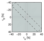
(a) (b)

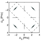
Figure 2: (a) A typical coincidence interferogram as a function of optical path differences $\tau_{A}$ and $\tau_{B}$ and (b) its Fourier transform. The dashed rectangle in (a) defines the scan range, which with suitable sampling density yields the region of interest in the frequency domain, outlined in (b).

Our experimental setup is depicted in the Fig. 3(a). The photon pairs were generated in a 1 mm thick nonlinear BBO crystal in a type-I process. The crystal was pumped by 100 fs long pulses centered at 390 nm, 20 mW average power and a repetition of 80 MHz. The ultraviolet beam was focused on the crystal to a spot measured to be 155 $\mu$m in diameter. The crystal was cut at $29.7^{\circ}$ to the optic axis, and oriented perpendicular to the pump beam. Two Mach-Zender interferometers MZ1 and MZ2 collected down-converted light at angles $1.28^{\circ}$ and $1.05^{\circ}$. The photons transmitted through the interferometers were coupled into single-mode fibers defining the spatial modes in which the down-conversion is collected.Dragan (2004) Finally the photons were detected using single photon counting modules SPCM connected to fast coincidence electronics and a PC controlled counter board.

In order to ensure the stability of the interferometric setup over the entire two-dimensional scan we used a pair of common path Mach-Zenders, in which the two arms were implemented as orthogonal polarization components while the optical path difference was modulated by a Soleil compensator, as depicted in Fig. 3(b). The generated photons entered from the left, with their polarization set to $45^{\circ}$ by the half-wave plate HWP. Then the photons went through a block of crystalline quartz QP with a vertical optic axis, and a pair of wedges QW with horizontal optic axes. With this setup, the sign and the value of the delay between the horizontal and vertical polarization components could be accurately controlled by sliding one of the wedges, mounted on the stepper motor driven translation stage, into the beam. Finally the two polarizations were brought to interference using a second half-wave plate HWP and a polarizing beam-splitter P, and the transmitted photons were coupled into a single-mode fiber F using aspheric lens L and detected. We verified that for the spectral range of interest birefringence dispersion could be neglected and consequently the delays $\tau_{i}$ were linearly dependent on the displacements of the quartz wedges. The quartz blocks used in the setup allowed to vary the delays from $-250$ fs to 250 fs.

(a)
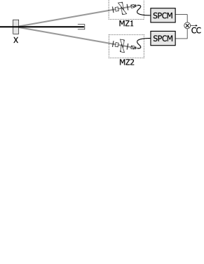
(b)

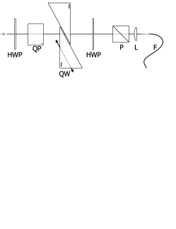
Figure 3: (a) Experimental setup. X, BBO crystal; MZ1, MZ2, Mach-Zender interferometers; SPCM, single photon counting module. (b) Common-path Mach-Zender interferometer. HWP, half-wave plate; QP, quartz plate; QW, quartz wedges; P, polarizer; L, aspheric lens; F, single-mode fiber.

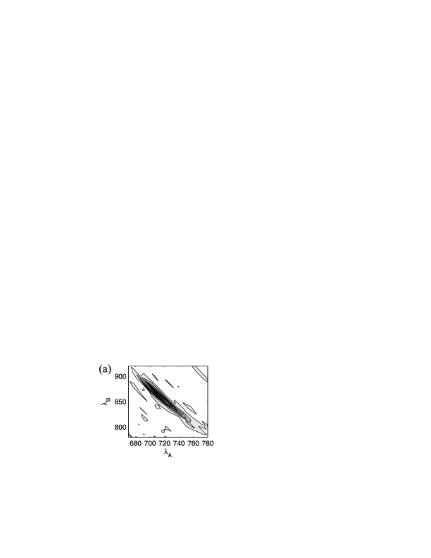
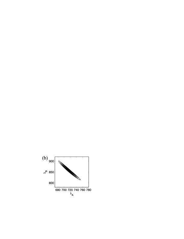
Figure 4: (a) Measured joint spectrum of photon pairs $\langle\mathop{:}\hat{I}_{A}(\lambda_{A})\hat{I}_{B}(\lambda_{B})\mathop{:}\rangle$ as a function of the wavelengths $\lambda_{A}$ and $\lambda_{B}$; (b) theoretical predictions of the joint spectral intensity; the cross-sections of the theoretical (dashed line) and the experimental (solid with dots marking errors) distributions along the lines (c) $\lambda_{A}^{-1}+\lambda_{B}^{-1}=\text{const}$ and (d) $\lambda_{A}^{-1}-\lambda_{B}^{-1}=\text{const}$ passing through the maximum.

The complete measurement consisted in a scan of a rectangular grid depicted in Fig. 1(a) spanned by 800$\times$40 points, where the first number refers to the direction perpendicular to the fringes. The corresponding mesh was 0.57 fs $\times$ 2 fs, and coincidences were counted for 3 s at each point. The reconstructed joint spectrum of photon pairs, normalized to unity, is depicted in Fig. 4(a). We compare it with theoretical calculations plotted in Fig. 4(b). The theoretical model used in these calculations assumed the exact phase matching function of the nonlinear crystal. The transverse components of the wave vectors for the pump and down-converted beams were treated in the paraxial approximation. The joint spectrum was calculated for coherent superpositions of plane-wave components of the down-conversion light that add up to localized spatial modes defined by the collecting optics and single-mode fibers. In order to facilitate a more quantitative comparison, Figs. 4(c) and (d) show the cross sections of the joint spectra along directions of maximum and minimum width in the frequency domain. In these plots, the experimental data have been interpolated between the points of the Fourier-domain grid, and presented together with statistical errors calculated assuming Poissonian noise affecting coincidence counts.

In summary, we proposed Fourier spectroscopy for measuring the joint spectrum of photons pairs, and demonstrated its application to down-converted light generated in a type-I BBO crystal. The result of the reconstruction agrees well with a careful theoretical calculation of the joint spectrum. We were able to reduce substantially the overall duration of the measurement by selecting the region of the interferogram which contains information about the relevant characteristics of the spectrum. Finally, let us note that compared to scanning spectrometers, Fourier spectroscopy exhibits higher signal-to-noise ratio when detection noise is dominated by an additive contribution. This effect, known as the multiplex advantage,Tai and Harwit (1976) is important in the case of high dark count rates, which is typical for single-photon measurements performed at telecom wavelengths.Gisin et al. (2002)

This research was in part supported by KBN grant number 2P03B 029 26 and it has been carried out in the National Laboratory for Atomic, Molecular, and Optical Physics in Toruń, Poland. P.W. gratefully acknowledges the support of the Foundation for Polish Science (FNP) during this work.

References

- Gisin et al. (2002) N. Gisin, G. Ribordy, W. Tittel, and H. Zbinden, Rev. Mod. Phys. 74, 145 (2002).
- Giovannetti et al. (2001) V. Giovannetti, S. Lloyd, and L. Maccone, Nature 412, 417 (2001).
- Valencia et al. (2004) A. Valencia, G. Scarcelli, and Y. Shih, Appl. Phys. Lett. 85, 2655 (2004).
- Nasr et al. (2003) M. B. Nasr, B. E. A. Saleh, A. V. Sergienko, and M. C. Teich, Phys. Rev. Lett. 91, 083601 (2003).
- Walther et al. (2005) P. Walther, K. J. Resch, T. Rudolph, E. Schenck, H. Weinfurter, V. Vedral, M. Aspelmeyer, and A. Zeilinger, Nature 434, 169 (2005).
- Kurtsiefer et al. (2001) C. Kurtsiefer, M. Oberparleiter, and H. Weinfurter, Phys. Rev. A 64, 023802 (2001).
- U’Ren et al. (2003) A. B. U’Ren, K. Banaszek, and I. A. Walmsley, Quant. Inf. Comput. 3, 480 (2003).
- König and Wong (2004) F. König and F. N. C. Wong, Appl. Phys. Lett. 84, 1644 (2004).
- Torres et al. (2005) J. P. Torres, F. Maciá, S. Carrasco, and L. Torner, Opt. Lett. 30, 314 (2005).
- Lee et al. (2005) P. S. K. Lee, M. P. van Exter, and J. P. Woerdman, Phys. Rev. A 72, 033803 (2005).
- Kim and Grice (2005) Y.-H. Kim and W. P. Grice, Opt. Lett. 30, 908 (2005).
- Dragan (2004) A. Dragan, Phys. Rev. A 70, 053814 (2004).
- Tai and Harwit (1976) M. H. Tai and M. Harwit, Appl. Opt. 15, 2664 (1976).