Linking Entanglement and Quantum Phase Transitions via Density Functional Theory

Abstract

Density functional theory (DFT) is shown to provide a novel conceptual and computational framework for entanglement in interacting many-body quantum systems. DFT can, in particular, shed light on the intriguing relationship between quantum phase transitions and entanglement. We use DFT concepts to express entanglement measures in terms of the first or second derivative of the ground state energy. We illustrate the versatility of the DFT approach via a variety of analytically solvable models. As a further application we discuss entanglement and quantum phase transitions in the case of mean field approximations for realistic models of many-body systems.

I Introduction

Density functional theory (DFT) HK:64 ; Kohn:65 is to date the most successful method for first principles calculations of the electronic properties of solids. The key to its success is a transformation of the dependence of the properties of a system of interacting particles on their single particle potential, to a dependence on the ground state density, thereby facilitating useful approximations of the many-body interaction for first principles computations. One rather relevant phenomenon in many-body physics is the ocurrence of quantum phase transitions (QPTs), which consist in critical changes in the properties of the ground state, driven purely by quantum fluctuations and effectively occurring at temperature $T=0$ Sachdev:book . QPTs are associated with level crossings, which usually lead to the presence of non-analyticities in the energy spectrum. Specifically, a first-order QPT (1QPT) is characterized by a finite discontinuity in the first derivative of the ground state energy. Similarly, a second-order QPT (2QPT) is characterized either by a finite discontinuity or divergence in the second derivative of the ground state energy, assuming the first derivative is continuous.

Many-body physics and, in particular, critical phenomena near QPTs, have recently been the subject of intense interest from the perspective of the theory of quantum information. A key observation is that, since entanglement describes correlations in a quantum system, its quantification may provide a convenient and precise description of a QPT. Indeed, entanglement has been found to exhibit scaling behavior near a critical point Osterloh:02 ; Osborne:02 ; Vidal:03 . Moreover, under well-delineated conditions and for distinguishable systems up to two-body interactions, a formal relationship between QPT and bipartite entanglement was recently established WuSarandyLidar:04 . Here, we show that entanglement may be well specified and conveniently computed within DFT. In DFT, any entanglement measure is a function(al) of the expectation values of the observables. This procedure introduces a direct connection between entanglement and the derivatives of the ground state energy of the quantum system with respect to the field coefficients, leading to a deep relationship between entanglement and QPT.

II Generalized Hohenberg-Kohn (HK) theorem and entanglement

Consider a quantum system described by a Hamiltonian composed of two parts

$$H=H_{0}+H_{\mathrm{ext}}=H_{0}+\sum_{l}\lambda_{l}\widehat{A}_{l},$$ (1)

where $\lambda_{l}$ is the “field coefficient” (control parameter) associated with a set of Hermitian operators $\{\widehat{A}_{l}\}$, e.g., an observable relevant to driving a quantum phase transition. The index $l$ can be discrete or continuous. The expectation values of $\widehat{A}_{l}$ for a ground state $\left|\psi\right\rangle$ are denoted by the set $\{a_{l}\}\equiv\{\left\langle\psi\right|\widehat{A}_{l}\left|\psi\right\rangle\}$.

DFT is originally based on the Hohenberg-Kohn (HK) theorem HK:64 . In the case of a many-electron system, the HK theorem establishes that the ground state electronic density $n(\mathbf{r})$, instead of the potential $v(\mathbf{r})$, can be used as the fundamental variable to describe the physical properties of the system. In the case of a Hamiltonian given by Eq. (1), the HK theorem can be generalized to the statement that there is a duality (in the sense of a Legendre transform) between the set of expectation values $\{a_{l}\}$ (corresponding to $n(\mathbf{r})$) and the set of field parameters $\{\lambda_{l}\}$ (corresponding to $v(\mathbf{r})$)  Schonhammer:95 . The commutativity of the densities at distinct points, $[\widehat{n}(\mathbf{r}),\widehat{n}(\mathbf{r}^{\prime})]=0$ for $\mathbf{r\neq r}^{\prime}$, is a property of the original HK theorem. In a lattice system, we require that the physical observables $\{A_{l}\}$ on different sites are mutually commuting operators. This allows not only different observables on the same site, e.g. $S^{x}_{l},S^{y}_{l}$, to be non-commutative, but also, for later use, endows a function of observables on different sites with a single site locality, such as the set of two site operators, $\{A_{l}A_{l+c}\}$, $l$ ranging over all sites and $c$ being a constant. It follows from the Legendre transform that the ground state expectation value of any observable can be interchangeably viewed as a unique function of either $\{\lambda_{l}\}$ or $\{a_{l}\}$. (See Appendix A for a simple proof of the HK theorem in a lattice). Such a general duality has allowed for the application of DFT in, e.g., interacting quantum spin systems Libero:03 . Moreover, as we show below, it can provide a natural connection between entanglement and QPT. Indeed, using the Hellmann-Feynman theorem Hellmann:37 ; Feynman:39 ,

$$\frac{\partial E}{\partial\lambda_{l}}=\left\langle\psi\right|\frac{\partial H}{\partial\lambda_{l}}\left|\psi\right\rangle=\left\langle\psi\right|\widehat{A}_{l}\left|\psi\right\rangle=a_{l}.$$ (2)

This means that the set of observables $\{{\partial H}/{\partial\lambda_{l}}\}$ has a direct linear relation with $\{a_{l}\}$. An example is the metallization of a semiconductor under pressure to a value at which the band gap given by the discontinuity of the density functional derivative of the ground state energy goes to zero Sham:83 ; Perdew:83 .

The HK theorem can be used to redefine entanglement measures in terms of new physical quantities: expectation values of observables, $\{a_{l}\}$, instead of external control parameters, $\{\lambda_{l}\}$. Consider an arbitrary entanglement measure $M$ for the ground state of Hamiltonian (1). We will focus here on bipartite entanglement, but our discussion applies equally well to multipartite measures. We then prove a central lemma, which very generally connects $M$ and energy derivatives.

Lemma. Any entanglement measure $M$ can be expressed as a unique functional of the set of first derivatives of the ground state energy:

$$M=M(\{a_{l}\})=M(\{\frac{\partial E}{\partial\lambda_{l}}\}),$$ (3)

assuming that the ground state is non-degenerate.

Proof. Intuitively, the proof follows from the fact that, according to the generalized HK theorem, any ground state wave function $|\Psi\rangle$ is a unique functional of $\{a_{l}\}$ and since $|\Psi\rangle$ provides a complete description of the state of the system, everything else is a unique functional of $\{a_{l}\}$ as well, including $M$. More formally, let us consider the case of pairwise entanglement of qubits. The case of higher dimensional systems or multipartite entanglement is a direct generalization. Then: (A) $M_{ij}$ (entanglement measure between qubits $i$ and $j$) is always a function $f$ of the matrix elements of the 2-qubit reduced density matrix $\rho_{ij}$: $M_{ij}=f(\rho_{ij})$. (B) The matrix elements $\rho_{ij}$ are combinations of correlation functions $\langle\sigma_{i}^{a}\sigma_{j}^{b}\rangle=\mathrm{Tr}(\sigma_{i}^{a}\sigma_{j}^{b}\rho_{ij})$, where $a,b=0,..,3$, with $\sigma_{0}=I$ (identity). This follows from an expansion of $\rho_{ij}$ in the Pauli basis $\{\sigma_{i}^{a}\sigma_{j}^{b}\}$. (C) From steps (A) and (B) it follows that $M=M(\langle\sigma_{i}^{a}\sigma_{j}^{b}\rangle)$. However, by using the HK theorem for non-degenerate ground states, any expectation value can be taken as a function of $\{a_{l}\}$, since the wave function itself is a function of $\{a_{l}\}$ (see, e.g., Ref. Schonhammer:95 ). Therefore, $M=M(\{a_{l}\})$, as required.   

In Ref. WuSarandyLidar:04 , relations similar to Eq. (3), which connects entanglement and 1QPTs, were established at the critical point for several examples of multi-particle systems, up to two-body interactions. In DFT, Eq. (3) holds for arbitrary systems, and not only close to the critical point. While the HK theorem is also applicable to degenerate ground states Levy:79 ; Kohn:85 , not all linear combinations of densities corresponding to degenerate ground states are permissible when implementing the variational principle Lieb:83 . Note also that systems described by either Fermi or Pauli operators can be considered using DFT. Indeed, the treatment of both cases can be unified by the Jordan-Wigner transformation Jordan:28 , with $H$, $H_{0}$, and $H_{\mathrm{ext}}$ expressed in terms of linear combinations of generators of $SU(2^{N})$, where $N$ denotes the number of sites in the case of spins in a lattice, or the number of single modes for Jordan-Wigner fermions.

Moreover, the HK theorem implies that one can split up the Hamiltonian (1) in different ways. For example, a new $H_{0}$ might include part of the sum $\sum\lambda_{l}\widehat{A}_{l}.$ In our discussion, it is often convenient to focus on one of the external operators by moving the others into $H_{0}$.

For 2QPTs, we should examine the derivatives of $M$. For simplicity of exposition, we regard one of the parameters $\lambda_{l}$ as an independent variable, which we denote by $\lambda$, and consider all the others as part of $H_{0}$. Therefore, $M$ can be seen as an exclusive function of $\lambda$, yielding via Eq. (2)

$$\frac{\partial M}{\partial\lambda}=\frac{\partial M}{\partial a}\frac{\partial a}{\partial\lambda}=\frac{\partial M}{\partial a}\frac{\partial^{2}E}{\partial\lambda^{2}}.$$ (4)

Notice that this equation holds only for non-degenerate ground states, since for the case of degeneracy, although the density $a$ still uniquely specifies the potential $\lambda$, the potential $\lambda$ does not uniquely specify the density $a$ anymore. Therefore, in the degenerate case, $a$ cannot be taken as a function of $\lambda$, which implies that the chain rule used to take the derivative in Eq. (4) is not valid. However, as long we restrict ourselves to non-degenerate states (as is the usual case for large finite systems tending to criticality), or approach the (critical) degeneracy point from below or above, this problem can be avoided. In the case where the degeneracy is symmetry driven, we could also circumvent this problem by observing that degenerate states can be split by a symmetry breaking term which is then allowed to tend to zero in the study of QPTs.

Eq. (4) shows that an entanglement measure is proportional to the second derivative of energy as long as ${\partial M}/{\partial a}\neq 0$. By using appropriate bipartite entanglement measures, 2QPTs have usually been identified so far through either non-analytic or vanishing values of ${\partial M}/{\partial\lambda}$ at the critical point. Both cases are contained in Eq. (4).

It should be emphasized that Eqs. (3) and (4) hold for any system described by the Hamiltonian (1) as long as DFT is valid, in the degeneracy sense discussed above. Around the critical points, the left and right limits of the two equations still hold even if the DFT is questionable at the critical point. Eqs. (3) and (4) can be seen as the basic equations for the relation between QPTs and entanglement.

III Example I: One-body external couplings

As a first example of the applicability of Eqs. (3) and (4), let us consider $H_{\mathrm{ext}}=\sum_{i}\overrightarrow{\lambda}_{i}\cdot\overrightarrow{\sigma}_{i}$, which represents a system of qubits acted upon via independent single-qubit control terms. According to DFT, the energy is a functional of matrix elements of one-spin reduced density matrices, i.e., $E=E(\{\overrightarrow{\rho}_{i}\})$, where $\overrightarrow{\rho}_{i}=\left\langle\psi\right|\overrightarrow{\sigma}_{i}\left|\psi\right\rangle=\overrightarrow{\bigtriangledown}_{i}E$ is the Bloch vector, with components $\rho_{i}^{\alpha}=\left\langle\psi\right|\sigma_{i}^{\alpha}\left|\psi\right\rangle$. We consider a bipartition of the system, splitting it up into two parts. Then, assuming that the system is in a pure state, we can use the linear entropy as a measure of block entanglement, which reads $L^{(d)}=[d/(d-1)](1-{\textrm{Tr}}\,\rho^{2})$, where $0\leq L^{(d)}\leq 1$ and $\rho$ denotes a $d\times d$-dimensional density matrix. Explicit computation of the block entanglement of one qubit (the $i$th) with the rest of system yields $L_{i}^{(2)}=1-\left|\overrightarrow{\rho}_{i}\right|^{2}=1-\overrightarrow{\bigtriangledown}_{i}E\cdot\overrightarrow{\bigtriangledown}_{i}E$, which is a function of the parameters $\overrightarrow{\lambda}$. In the case of fermions, we replace the Pauli matrices by fermionic operators according to the Jordan-Wigner transformation. Then, $L_{i}^{(2)}=1-(\partial E/\partial\lambda_{zi})^{2}$ (number conservation law for fermions implies the vanishing of $\partial E/\partial\lambda_{xi}$ and $\partial E/\partial\lambda_{yi}$).

In the case of a 1QPT, characterized by a discontinuity in $\overrightarrow{\bigtriangledown}_{i}E$, we have a corresponding discontinuity in $L_{i}^{(2)}$ unless $\overrightarrow{\bigtriangledown}_{i}E\cdot\overrightarrow{\bigtriangledown}_{i}E$ is continuous. Therefore, in this case, when all $\overrightarrow{\lambda}_{i}$ are taken as independent external parameters, the entanglement measure $L_{i}^{(2)}$ is an analytic function of the first derivatives of the energy, yielding a natural relationship between 1QPTs and $L_{i}^{(2)}$. A general discussion of 2QPTs is, on the other hand, not as straigthforward, since the structure of the derivatives of $L_{i}^{(2)}$ will depend on the details of the model. Thus, it turns out to be more useful to analyze a concrete example. Let us consider the transverse field Ising chain, where $H=-\sum_{i=1}^{N}(\sigma_{i}^{x}\sigma_{i+1}^{x}+\lambda\sigma_{i}^{z})$, with $N$ denoting the number of spins along the chain and with cyclic boundary conditions assumed. In this model, a discussion of entanglement as a function of the coupling $\lambda$ was first presented in Refs. Osterloh:02 ; Osborne:02 . Due to translational symmetry we have $\rho_{z}=\left\langle\psi\right|\sigma^{z}\left|\psi\right\rangle=\frac{\partial\varepsilon}{\partial\lambda}$, where $\varepsilon=E/N$. Therefore $\frac{\partial L^{(2)}}{\partial\lambda}=\frac{\partial L^{(2)}}{\partial\rho_{z}}\frac{\partial^{2}\varepsilon}{\partial\lambda^{2}}$. Divergence of ${\partial^{2}\varepsilon}/{\partial\lambda^{2}}$ at the quantum critical point $\lambda=1$ will thus result in that of ${\partial L^{(2)}}/{\partial\lambda}$ unless ${\partial L^{(2)}}/{\partial\rho_{z}=0}$, which is not the case in this example. This is demonstrated in Fig. 1, where we plot $L^{(2)}$ as a function of $\rho_{z}$. Both the maximum and the singularity of the derivative occur at the critical point. We can also apply the DFT approach to pairwise entanglement measures. For instance, let us consider entanglement between nearest-neighbor pairs in the transverse field Ising model as measured by the negativity $\mathcal{N}$ Vidal:02a . From Eq. (4) we have $\frac{\partial\mathcal{N}}{\partial\lambda}=\frac{\partial\mathcal{N}}{\partial\rho_{z}}\frac{\partial^{2}\varepsilon}{\partial\lambda^{2}}$. Notice that the divergence in ${\partial^{2}\varepsilon}/{\partial\lambda^{2}}$ at the critical point naturally leads to a divergence in ${\partial\mathcal{N}}/{\partial\lambda}$, since ${\partial\mathcal{N}}/{\partial\rho_{z}}$ is a non-vanishing function at the QPT, as shown in Fig. 2. In fact, the maximum of ${\partial\mathcal{N}}/{\partial\rho_{z}}$ approaches the critical point as the number of sites increases.

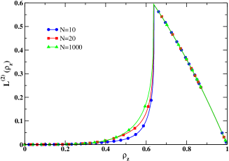
Figure 1: Block entanglement $L^{(2)}$ as function of $\rho_{z}$ for the transverse field Ising model. The maximum occurs at the quantum critical point, where $\rho_{z}\approx 0.6366$.

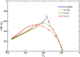
Figure 2: Derivative of the negativity with respect to $\rho_{z}$ for the transverse field Ising model. The maximum approaches the quantum critical point, where $\rho_{z}\approx 0.6366$.

IV Example II: two-body external couplings

In the case of two-body external couplings, we take $H_{\mathrm{ext}}=\sum_{ij}\lambda_{ij}^{\alpha}\sigma_{i}^{\alpha}\sigma_{j}^{\alpha}$, where $\alpha\in\{x,y,z\}$. This Hamiltonian represents a system of qubits controlled externally via two-body interactions. Entanglement between qubits $i,j$ and the rest of the system can then be computed by taking the linear entropy $L^{(d)}$ for $d=4$. This yields $L^{(4)}=1-\frac{1}{3}\sum(\frac{\partial E}{\partial\lambda_{ij}^{\alpha}})^{2}$. We now analyze the behavior of $L^{(4)}$ in some important models exhibiting QPTs. For example, for the XXZ spin chain, we have $H=(-1/2)\sum_{i}^{N}(\sigma_{i}^{x}\sigma_{i+1}^{x}+\sigma_{i}^{y}\sigma_{i+1}^{y}+\Delta\sigma_{i}^{z}\sigma_{i+1}^{z})$, where cyclic boundary conditions are assumed. The external Hamiltonian is taken as $H_{\mathrm{ext}}=-(\Delta/2)\sum_{i}\sigma_{i}^{z}\sigma_{i+1}^{z}$. Direct evaluation of $L^{(4)}$ then yields (See Appendix B)

$$L^{(4)}=1-\frac{4}{3}\left[\left(1+\frac{\Delta^{2}}{2}\right)\left(\frac{\partial\varepsilon}{\partial\Delta}\right)^{2}+\frac{\varepsilon^{2}}{2}-\varepsilon\Delta\frac{\partial\varepsilon}{\partial\Delta}\right],$$ (5)

where $\varepsilon=E/N$. Notice that $L^{(4)}$ is a function of the DFT variable $a=\langle\sigma_{i}^{z}\sigma_{i+1}^{z}\rangle=-2(\partial\varepsilon/\partial\Delta)$ since, due to the HK theorem, the energy density $\varepsilon$ can be taken as a function of $a$. Thus, discontinuities in $(\partial\varepsilon/\partial\Delta)$ will be directly reflected in $L^{(4)}$. This model exhibits two distinct QPTs, which occur at $\Delta=1$ and $\Delta=-1$. In order to evaluate $L^{(4)}$, we consider the ground state wave-function with vanishing magnetization, which favors the presence of entanglement in the system. A 1QPT occurs at $\Delta=1$, which separates a ferromagnetic phase from a gapless quasi-long-range-ordered phase. At this ferromagnetic critical point, the energy density as $N\rightarrow\infty$ is continuous, and is given by $\varepsilon(\Delta=1)=-1/2$ Yang:66a ; Yang:66b . However, its first derivative is discontinuous, with $(\partial\varepsilon/\partial\Delta)_{\Delta\rightarrow 1^{+}}\rightarrow-1/2$ and $(\partial\varepsilon/\partial\Delta)_{\Delta\rightarrow 1^{-}}\rightarrow 0$. From Eq. (5), we can see that this discontinuity is immediately manifested in the entanglement measure, since $L^{(4)}$ jumps from $2/3$ to $5/6$ at $\Delta=1$. A continuous QPT in the XXZ chain occurs at $\Delta=-1$, separating the gapless quasi-long-range-ordered phase from the antiferromagnetic phase. For this case, it is useful to compute the first derivative of $L^{(4)}$ with respect to $\Delta$, which yields $({\partial L^{(4)}}/{\partial\Delta})=({\partial L^{(4)}}/{\partial a})({\partial^{2}\varepsilon}/{\partial\Delta^{2}})$, with $\frac{\partial L^{(4)}}{\partial a}=\frac{4}{3}\left[\varepsilon\Delta-2\left(1+\frac{\Delta^{2}}{2}\right)\frac{\partial\varepsilon}{\partial\Delta}\right]$. The QPT in this case is not directly signalled by $({\partial^{2}\varepsilon}/{\partial\Delta^{2}})$, which is analytic at $\Delta=-1$ Yang:66a ; Yang:66b . However, entanglement detects this transition as an extremum at the critical point Gu:03 ; Chen:04 ; Yang:05 . This behavior is also reflected in terms of the DFT variable $a$. We have $\varepsilon(\Delta=-1)=2(\ln{2}-1/4)$ Yang:66a ; Yang:66b , and find for the first derivative of the energy $(\partial\varepsilon/\partial\Delta)_{\Delta\rightarrow-1}\approx 0.2954$. Therefore, we obtain $({\partial L^{(4)}}/{\partial a})=({\partial L^{(4)}}/{\partial\Delta})=0$.

We now analyze the behavior of $L^{(4)}$ in a Fermi system. An interesting example is then the one-dimensional Hubbard model, $H_{\mathrm{ext}}=U\sum_{\alpha}n_{\alpha\uparrow}n_{\alpha\downarrow}$, where $n_{\alpha\downarrow}~{}(n_{\alpha\uparrow})$ is the spin down (up) electronic number at site $\alpha$. The Hubbard model describes a metal-insulating transition, which has been considered from the point of view of entanglement in Refs. Gu:04 ; Larsson:05 . We can rearrange the indices for the modes $\alpha\uparrow$ and $\alpha\downarrow$ into nearest neighbor indices $i$ and $i+1$, respectively, in a linear lattice. Therefore, the Hamiltonian can be written as $H_{\mathrm{ext}}=U\sum_{i}n_{2i-1}n_{2i}$ where only the pairs of sites (1,2), (3,4), etc., interact with each other. We can then compute $L^{(4)}$ between an interacting pair $(i,i+1)$ and the rest of the system (see also Refs. Gu:04 ; Larsson:05 ). At half-filling, $L^{(4)}=\frac{2}{3}(1+4a-8a^{2})$ (for any $i$) (See Appendix C). Then $\frac{\partial L^{(4)}}{\partial a}=\frac{2}{3}(4-16a)$. By using Eq. (4), we obtain $\frac{\partial L^{(4)}}{\partial U}=\frac{\partial L^{(4)}}{\partial a}\frac{\partial^{2}\varepsilon}{\partial U^{2}}$. At the critical point $U=0$, which separates an insulating phase from a metallic phase, the first derivative of $L^{(4)}$ with respect to $U$ is ${\partial L^{(4)}}/{\partial U}=0$ Gu:04 . In terms of the new variable $a$, we can show that the QPT in the Hubbard model is also identified via an extremum of $L^{(4)}$. Indeed, for $U=0$, we have $a=1/4$ Economou:79 which then implies $\partial_{a}L^{(4)}=0$.

V The Lipkin model: a Hartree-Fock approach to entanglement

Most realistic physical many-body problems cannot be solved analytically. Linear approximations, such as Hartree-Fock-Bogoliubov theory and the random phase approximation, are often practical and effective ways to treat these systems, since these procedures change an intractable $2^{N}$-dimensional problem to a tractable $N^{2}$-dimensional one. In this case, it is appealing to introduce new and simple quantities, e.g., $L^{(2)}$ and $L^{(4)}$, as measures characterizing the quantum information content of these known approximate wave functions. We expect these quantities to become as important as, e.g., binding energies, when quantum information becomes readily accessible to experiments.

As an example, we consider the Lipkin model – important, e.g., in nuclear physics – whose Hamiltonian reads $H=\lambda S_{z}-\frac{1}{N}(S_{x}^{2}-S_{y}^{2})$, where $S_{z}=\sum_{m=1}^{N}\frac{1}{2}(c_{+m}^{\dagger}c_{+m}-c_{-m}^{\dagger}c_{-m})$ and $S_{x}+iS_{y}=\sum_{m=1}^{N}c_{+m}^{\dagger}c_{-m}$ Ring:book (for a discussion of entanglement in the Lipkin model, see also Ref. Vidal:04 ). This Hamiltonian describes a two-level Fermi system $\{|+\rangle,|-\rangle\}$, each level having degeneracy $N$. The operators $c_{+m}^{\dagger}$ and $c_{-m}^{\dagger}$ create a particle in the upper and lower levels, respectively. Alternatively, the Hamiltonian may be viewed as a one-dimensional ring of two-level atoms with infinite range interaction between pairs. The factor $1/N$ in the interaction term keeps the scaling of both terms in $H$ linear in $N$. The phase transition studied is in the limit of $N\rightarrow\infty$. The Lipkin model is exactly solvable (see, e.g., Ref. Ortiz:05 ). The Hartree-Fock (HF) ground state, which is exact for this model as $N$ tends to infinity, is given by $|HF\rangle=\prod_{m=1}^{N}a_{0m}^{\dagger}|-\rangle$, where $a_{0m}^{\dagger}$ is defined by the following change of variables: $c_{+m}^{\dagger}=\sin{\alpha}\,a_{0m}^{\dagger}+\cos{\alpha}\,a_{1m}^{\dagger}$ and $c_{-m}^{\dagger}=\cos{\alpha}\,a_{0m}^{\dagger}-\sin{\alpha}\,a_{1m}^{\dagger}$. The variational parameter $\alpha$ which yields the minimum energy is given by $\cos{2\alpha}=\lambda$ when $\lambda<1$ and $\alpha=0$ when $\lambda\geq 1$. We define the DFT variable $a=\partial\varepsilon/\partial\lambda$, with $\varepsilon=E/N$ denoting the energy per particle. For the HF ground state, we then obtain $a=-\frac{\lambda}{2}$ for $\lambda<1$ and $a=-\frac{1}{2}$ for $\lambda\geq 1$ It is easy to show that $\partial^{2}\varepsilon/\partial\lambda^{2}$ is discontinuous at $\lambda=1$, which corresponds to $a=-1/2$ in terms of the DFT variable. Let us analyze whether this discontinuity is reflected in the derivatives of the entanglement measures, as given by Eq. (4). For $4$-dimensional block entanglement, it is convenient to consider the entanglement between a block composed of two general modes ($+m$,$-n$) and the rest of the system, which yields $L_{+m,-n}^{(4)}=(2/3)(1-4a^{2})(1-\delta_{m,n})$, where $\delta_{m,n}$ is the Kronecker symbol. Therefore, the block ($+m,-n$) is entangled with the rest of system only if $m\neq n$. Taking the derivative, we obtain $(\partial L_{+m,-n}^{(4)}/\partial a)_{a=-1/2}=8/3$ $(m\neq n)$. Therefore, from Eq. (4), the non-analyticity of $\partial^{2}\varepsilon/\partial\lambda^{2}$ at the critical point will be associated to a non-analyticity in $\partial L_{+m,-n}^{(4)}/\partial\lambda$ ($m\neq n$). A similar result follows in the case of $2$-dimensional block entanglement, where we have $L^{(2)}=1-4a^{2}$ for a general mode $+m$ (or $-m$) with the rest of the system. Pairwise entanglement between general modes $+m$ and $-n$ as measured by the negativity is found to be $\mathcal{N}_{+m,-n}=\sqrt{1-4a^{2}}\delta_{m,n}$. Notice that this is in contrast with block entanglement, where modes $+m$ and $-n$ only are entangled for $m\neq n$. This difference is due to the structure of the HF ground state, which implies that the modes $+m$ and $-n$ interact only for $m=n$. Therefore, bipartite entanglement in the system appears only when $+m$ and $-m$ are in different parts. Evaluating now the derivative of the negativity we obtain $(\partial\mathcal{N}_{+m,-n}/\partial a)_{a\rightarrow-1/2}\rightarrow\infty$. Thus, $\partial\mathcal{N}_{+m,-n}/\partial\lambda$  is non-analytic at the critical point.

VI Conclusion

We have shown in general and illustrated in a number of models that DFT provides a natural link between entanglement and QPTs. Since experimental data are taken at finite temperature, it is important to be able to delineate the temperature fluctuation around a classical critical point versus the quantum fluctuations around a QPT. The exploration of finite-temperature DFT Mermin for the connection between phase transitions and quantum information appears to be a promising direction for future study.

Appendix A

We provide here a proof of the HK theorem in a lattice, based on the variational method (for a proof based on the constrained-search technique Levy:79 , see Ref. Schonhammer:95 ). Let us consider two sets of parameters $\{\lambda_{l}\}$ and $\{\lambda_{l}^{\prime}\}$, which define two Hamiltonians as follows:

$$H=H_{0}+\sum_{l}\lambda_{l}A_{l}\,\,,\,\,\,\,\,\,\,H^{\prime}=H_{0}+\sum_{l}\lambda_{l}^{\prime}A_{l}.$$ (6)

The ground states of $H$ and $H^{\prime}$ will be denoted by $|\psi\rangle$ and $|\psi^{\prime}\rangle$, respectively, which are taken as non-degenerate, even though the proof can be extended for degenerate ground states Levy:79 ; Kohn:85 . We also assume here that, for different sets of parameters, $\{\lambda_{l}\}\neq\{\lambda_{l}^{\prime}\}$, we have independent ground states $|\psi\rangle\neq\alpha|\psi^{\prime}\rangle$ ($\alpha=$ constant). This is indeed the usual behavior of quantum systems around criticality, where the ground state varies continuously as we vary the control parameters. By applying the variational principle for the Hamiltonian $H^{\prime}$, we obtain

$$\langle\psi^{\prime}|H^{\prime}|\psi^{\prime}\rangle<\langle\psi|H^{\prime}|\psi\rangle=\langle\psi|\left(H+\sum_{l}\left(\lambda_{l}^{\prime}-\lambda_{l}\right)A_{l}\right)|\psi\rangle$$ (7)

Therefore, Eq. (7) yields

$$E_{0}^{\prime}<E_{0}+\sum_{l}\left(\lambda_{l}^{\prime}-\lambda_{l}\right)a_{l},$$ (8)

where $E_{0}^{\prime}$ and $E_{0}$ are the ground state energies of $H^{\prime}$ and $H$, respectively, and $a_{l}=\langle\psi|A_{l}|\psi\rangle$. Analogously, by applying the variational principle for $H$, we obtain

$$E_{0}<E_{0}^{\prime}+\sum_{l}\left(\lambda_{l}-\lambda_{l}^{\prime}\right)a_{l}^{\prime},$$ (9)

with $a_{l}^{\prime}=\langle\psi^{\prime}|A_{l}|\psi^{\prime}\rangle$. From Eqs. (8) and (9) we have

$$0<\sum_{l}\left(\lambda_{l}^{\prime}-\lambda_{l}\right)\left(a_{l}-a_{l}^{\prime}\right)$$ (10)

Hence, if the sets of parameters $\{\lambda_{l}\}$ and $\{\lambda_{l}^{\prime}\}$ are different from each other, then we cannot have identical sets $\{a_{l}\}$ and $\{a_{l}^{\prime}\}$. Therefore, the density $\{a_{l}\}$ uniquely specifies the potential $\{\lambda_{l}\}$ and can then be used as the basic variable to describe the properties of the system.

Appendix B

We provide here the basic details of the evaluation of the linear entropy for the XXZ model. The density matrix for a pair of nearest-neighbor sites in the ground state of the XXZ chain can be written as

$$\mathcal{\rho}=\left(\begin{array}[]{cccc}A&0&0&0\\ 0&B&C&0\\ 0&C&B&0\\ 0&0&0&D\end{array}\right),$$ (11)

where, from the XXZ Hamiltonian, we obtain

$$A = D=\frac{1}{4}\left(1-2\frac{\partial\varepsilon}{\partial\Delta}\right),\,\,\,\,\,B=\frac{1}{4}\left(1+2\frac{\partial\varepsilon}{\partial\Delta}\right),$$

$$C = -\frac{1}{2}\left(\varepsilon-\Delta\frac{\partial\varepsilon}{\partial\Delta}\right).$$ (12)

Eqs. (12) allows for a direct calculation of the linear entropy $L^{(4)}=(4/3)(1-{\textrm{Tr}}\rho^{2})$, yielding the result displayed in Eq. (5).

Appendix C

We provide here the basic details for the evaluation of the linear entropy in the Hubbard model. Translation invariance and simultaneous conservation of particle number $N=\sum_{j}\left(n_{j\uparrow}+n_{j\downarrow}\right)$ and $z$-component of total spin $S^{z}=\sum_{j}\left(n_{j\uparrow}-n_{j\downarrow}\right)$ imply that the density operator for any single site can be represented by a $4\times 4$ diagonal matrix, whose eigenvalues are given by

$$w=\langle n_{\alpha\uparrow}n_{\alpha\downarrow}\rangle=\frac{\partial\varepsilon}{\partial U}\equiv a,\,\,\,\,u^{+}=\langle n_{\alpha\uparrow}\rangle-w,$$

$$u^{-}=\langle n_{\alpha\downarrow}\rangle-w,\,\,\,\,z=1-u^{+}-u^{-}-w.$$ (13)

At half-filling, we have $\langle n_{\alpha\uparrow}\rangle=\langle n_{\alpha\downarrow}\rangle=1/2$. Therefore, in this regime, all the eigenvalues can be expressed in terms of the density $a=\langle n_{\alpha\uparrow}n_{\alpha\downarrow}\rangle$. Then, the evaluation of the linear entropy $L^{(4)}(a)$ follows straightforwardly.

References

- (1) P. Hohenberg and W. Kohn, Phys. Rev. 136, B864 (1964).
- (2) W. Kohn and L. J. Sham, Phys. Rev. 140, A1133 (1965).
- (3) S. Sachdev, Quantum Phase Transitions (Cambridge University Press, Cambridge, UK, 2001).
- (4) A. Osterloh, L. Amico, G. Falci, and R. Fazio, Nature 416, 608 (2002).
- (5) T. J. Osborne and M. A. Nielsen, Phys. Rev. A 66, 032110 (2002).
- (6) G. Vidal, J. I. Latorre, E. Rico, and A. Kitaev, Phys. Rev. Lett. 90, 227902 (2003).
- (7) L.-A. Wu, M. S. Sarandy, and D. A. Lidar, Phys. Rev. Lett. 93, 250404 (2004).
- (8) K. Schonhammer, O. Gunnarsson, and R. M. Noack, Phys. Rev. B 52, 2504 (1995).
- (9) V. L. Líbero and K. Capelle, Phys. Rev. B 68, 024423 (2003).
- (10) H. Hellmann, Die Einführung in die Quantenchemie (Deuticke, Leipzig, 1937).
- (11) R. P. Feynman, Phys. Rev. 56, 340 (1939).
- (12) L. J. Sham and M. Schlüter, Phys. Rev. Lett. 51, 1888 (1983).
- (13) J. P. Perdew and M. Levy, Phys. Rev. Lett. 51, 1884 (1983).
- (14) P. Jordan and E. Wigner, Z. Phys. 47, 631 (1928).
- (15) M. Levy, Proc. Natl. Acad. Sci. 76, 6062 (1979).
- (16) W. Kohn, Highlights of Condensed- Matter Theory, Soc. Italiana di Fisica, Bologna, Italy, LXXXIX, Corso, 1985.
- (17) E. H. Lieb, Int. J. Quant. Chem. 24, 243 (1983).
- (18) G. Vidal and R. F. Werner, Phys. Rev. A 65, 032314 (2002).
- (19) C. N. Yang and C. P. Yang, Phys. Rev. 150, 321 (1966).
- (20) C. N. Yang and C. P. Yang, Phys. Rev. 150, 327 (1966).
- (21) S.-J. Gu, H.-Q. Lin, and Y.-Q. Li, Phys. Rev. A 68, 042330 (2003).
- (22) Y. Chen, P. Zanardi, Z. D. Wang, and F. C. Zhang, New J. Phys. 8, 97 (2006).
- (23) M.-F. Yang, Phys. Rev. A 71, 030302(R) (2005).
- (24) S.-J. Gu, Y.-Q Li, and H.-Q. Lin, Phys. Rev. Lett. 93, 086402 (2004).
- (25) D. Larsson and H. Johannesson, Phys. Rev. Lett. 95, 196406 (2005).
- (26) E. N. Economou and P. N. Poulopoulos, Phys. Rev. B 20, 4756 (1979).
- (27) P. Ring and P. Schuck, The Nuclear Many-Body Problem (Springer-Verlag, New York, 1980).
- (28) J. Vidal, G. Palacios, and C. Aslangul, Phys. Rev. A 70, 062304 (2004).
- (29) G. Ortiz, R. Somma, J. Dukelsky, and S. Rombouts, Nucl. Phys. B 707, 421 (2005).
- (30) N. D. Mermin, Phys. Rev. 137, A1441 (1965).