NON-INTEGER QUANTUM TRANSITIONS

Abstract

We show that in the quantum transition of a system induced by the interaction with an intense laser of circular frequency $\omega$, the energy difference between the initial and the final states of the system is not necessarily being an integer multiple of the quantum energy $\hbar\omega$.

PACS: 03.65.-w, 32.80.Fb, 32.90.+a, 33.60.-q

Keywords: Transitions induced by intense lasers, Non-perturbation effect, Violation of Bohr condition

1 Introduction

It is widely accepted that the Bohr condition

$$E_{2}-E_{1}=\pm\hbar\omega$$ (1)

expresses the energy conservation in the quantum transition from the state with energy $E_{1}$ to the state with energy $E_{2}$, induced by the interaction of the system with the electromagnetic field of circular frequency $\omega$. It may be generalized to

$$E_{2}-E_{1}=N\hbar\omega\;,$$ (2)

with an integer $N$, when the system is interacting with a laser. This generalized Bohr condition is still thought to be an expression of the energy conservation in the transition, with the number of absorbed or emitted photons being more than 1. The transitions satisfying (2) with $N>1$ had been observed experimentally in forms of the multi-photon ionization (MPI)[1] and the above threshold ionization (ATI)[2] . Here, we would emphasize that the Bohr condition (1) or (2) is approximate, and its energy conservation interpretation is not exact either. As we know, every spectrum line has its width. It means there is always an error when (1) is applied to an individual transition. It becomes specially obvious when we apply it to the magnetic resonances. In this case, the resonance frequency is determined by a constant magnetic field, and the width of resonance is determined by a rotating magnetic field. The strengths of these two fields are comparable. It means, in most individual magnetic transitions the Bohr condition (1) is seriously violated. However, the violation of Bohr condition does not mean the violation of energy conservation. Since the energy conservation means that the total energy of the system and the electromagnetic fields does not change, but the sum of the energy of the system and that of the electromagnetic fields is not the total energy. Their difference is the interaction energy between the system and the electromagnetic fields. Only when this difference is negligible, the Bohr condition becomes a good approximation of energy conservation, and therefore has to be fulfilled. In this case the interaction energy may be regarded as a perturbation. It is realized for the transitions in weak fields. In the following, we shall see, for the transitions in lasers, Bohr condition may be badly violated. For an individual transition we always have

$$E_{2}-E_{1}=\eta\hbar\omega\;,$$ (3)

with $\eta$ being defined in it. For transitions in strong electromagnetic fields, like in lasers, $\eta$ may be quite different from any integer. We call this kind of transition a non-integer quantum transition.

Therefore, Bohr condition is not a first principle, but a special relation for special processes. It may be deduced from quantum mechanics by perturbation. (2) is a result of the limit

$$\lim_{t\rightarrow\infty}\frac{\sin^{2}[(E_{2}-E_{1}-N\hbar\omega)\frac{t}{2\hbar}]}{(E_{2}-E_{1}-N\hbar\omega)^{2}\frac{t}{2\hbar}}=\pi\delta(E_{2}-E_{1}-N\hbar\omega)$$ (4)

in the $N$th order perturbation, showing that the Bohr condition is a representation of the resonance with an integer $N$. In a strong electromagnetic field, the interaction energy between the system and the field is large. The quantum transition has to be handled by non-perturbation method. This kind of resonance may not appear and the non-integer quantum transition appears. It is a non-perturbation effect.

2 Transitions between discrete levels, laser Raman effects

A laser is a classical limit of the intense electromagnetic wave. In the Coulomb gauge, the circularly polarized laser is therefore well described by the vector potential

$${\textit{{A}}}=A[{\textit{{x}}}_{0}\cos(kz-{\omega}t)+{\textit{{y}}}_{0}\sin(kz-{\omega}t)]\ .$$ (5)

Consider the quantum transition of a hydrogen atom irradiated by this laser. At the moment, we would simplify the problem to the motion of a non-relativistic spin-less electron in the Coulomb field and the laser. Possible corrections of the omitted effects on the result will be discussed in section 4. The Hamiltonian of this electron is

$$\hat{H}=\hat{H}_{0}+\hat{H}^{\prime}\ ,$$ (6)

with

$$\hat{H}_{0} = \frac{\hat{p}^{2}}{2m}+V(r)\ ,$$ (7)

$$\hat{H}^{\prime} = \frac{eA}{m}[\hat{p}_{x}\cos(kz-\omega t)+\hat{p}_{y}\sin(kz-\omega t)]+\frac{e^{2}A^{2}}{2m}\ .$$ (8)

$V(r)=-\alpha\hbar c/r$ is the Coulomb potential for the electron, $\alpha$ is the fine structure constant, $-e$ and $m$ are the electric charge and mass of the electron respectively. The Schrödinger equation

$${\rm i}\hbar\frac{\partial\Psi}{\partial t}=\hat{H}\Psi$$ (9)

for the electron is time dependent. However, a transformation

$$\Psi({\textit{{r}}},t)={\rm e}^{{\rm i}\omega\hat{L}_{z}t/\hbar}\Phi({\textit{{r}}},t)$$ (10)

changes it into a time independent pseudo-Schrödinger equation

$${\rm i}\hbar\frac{\partial\Phi}{\partial t}=\hat{H}_{\rm ps}\Phi\ ,$$ (11)

with the pseudo-Hamiltonian

$$\hat{H}_{\rm ps}=\hat{H}_{0}^{\prime}+\hat{H}^{\prime\prime}\ ,$$ (12)

in which

$$\hat{H}_{0}^{\prime}=\hat{H}_{0}+\omega\hat{L}_{z}\;\;\;\;\mbox{and}\;\;\;\;\hat{H}^{\prime\prime}=\frac{eA}{m}[\hat{p}_{x}\cos(kz)+\hat{p}_{y}\sin(kz)]+\frac{e^{2}A^{2}}{2m}$$ (13)

are time independent. Denote the $i$th eigenfunction of $\hat{H}_{\rm ps}$ by $\phi_{i}({\textit{{r}}})$. We have

$$\hat{H}_{\rm ps}\phi_{i}({\textit{{r}}})=E_{i}\phi_{i}({\textit{{r}}})\ ,$$ (14)

$E_{i}$ is the pseudo-energy of the electron in the pseudo-stationary state $\phi_{i}({\textit{{r}}})$. They may be quite different from the energy $E_{n}=-\alpha^{2}mc^{2}/2n^{2}$ and the stationary state

$$\psi_{nl\mu}({\textit{{r}}})=\frac{{\rm i}^{l}}{(2l+1)!}\left[\left(\frac{1}{na_{0}}\right)^{2l+3}\frac{(n+l)!}{2n(n-l-1)!}\right]^{1/2}{\rm e}^{-\frac{r}{na_{0}}}r^{l}{\rm F}(l+1-n,2l+2,\frac{2r}{na_{0}}){\rm Y}_{l\mu}(\theta\varphi)$$ (15)

of the electron in an isolated hydrogen atom respectively. $a_{0}$ is the Bohr radius, F is the confluent hypergeometric function, and Y is the spherical harmonic function. $r,\theta$ and $\varphi$ are spherical coordinates of the electron. Now, let us expand $\phi_{i}$ in terms of the wave functions [$\psi_{nl\mu}$]:

$$\phi_{i}({\textit{{r}}})=\sum_{nl\mu}C_{nl\mu}(i)\psi_{nl\mu}({\textit{{r}}})\ .$$ (16)

This is an approximation, since the set [$\psi_{nl\mu}$] of bound states only is not complete. We expect that it is good enough for the state $\phi_{i}$ near a low lying bound state. We further assume that in the expansion (16) only terms with $n\leq n_{0}$ are important, therefore one may truncate the summation on the right at $n=n_{0}$. This makes the eigen-equation (14) become an linear algebraic equation, and therefore may be solved by the standard method[3].

The factor ${\rm i}^{l}$ on the right of (15) makes the matrix elements of $\hat{H}_{\rm ps}$ be real in the $\hat{H}_{0}^{\prime}$ representation . Therefore the solutions $[C_{nl\mu}(i)]$ are real. We have the reciprocal expansion

$$\psi_{nl\mu}({\textit{{r}}})=\sum_{i}C_{nl\mu}(i)\phi_{i}({\textit{{r}}})\ .$$ (17)

Suppose the hydrogen atom stays in the state $\psi_{nl\mu}$ when $t\leq 0$. The laser arrives at $t\!=\!0$. According to (10), (11) and (14), at $t>0$, the pseudo-state will be

$$\Phi({\textit{{r}}},t)=\sum_{i}C_{nl\mu}(i)\phi_{i}({\textit{{r}}}){\rm e}^{-{\rm i}E_{i}t/\hbar}=\sum_{n^{\prime}l^{\prime}\mu^{\prime}}\sum_{i}C_{nl\mu}(i)C_{n^{\prime}l^{\prime}\mu^{\prime}}(i){\rm e}^{-{\rm i}E_{i}t/\hbar}\psi_{n^{\prime}l^{\prime}\mu^{\prime}}({\textit{{r}}})\ ,$$ (18)

and the state becomes

$$\Psi({\textit{{r}}},t)=\sum_{n^{\prime}l^{\prime}\mu^{\prime}}\sum_{i}C_{nl\mu}(i)C_{n^{\prime}l^{\prime}\mu^{\prime}}(i){\rm e}^{-{\rm i}(E_{i}-\mu^{\prime}\hbar\omega)t/\hbar}\psi_{n^{\prime}l^{\prime}\mu^{\prime}}({\textit{{r}}})\ .$$ (19)

The transition probability of the hydrogen atom from the state $\psi_{nl\mu}$ to the state $\psi_{n^{\prime}l^{\prime}\mu^{\prime}}$ is

$$w_{n^{\prime}l^{\prime}\mu^{\prime};nl\mu}(t)=\left|\sum_{i}C_{nl\mu}(i)C_{n^{\prime}l^{\prime}\mu^{\prime}}(i){\rm e}^{-{\rm i}(E_{i}-\mu^{\prime}\hbar\omega)t/\hbar}\right|^{2}\ .$$ (20)

It is a multi-periodic function of $t$. The periods are of the microscopic order of magnitude. On the other hand, the observation is done in a macroscopic duration. Therefore the observed transition probability is a time average of (20) over its periods. The averages of the cross terms with different $i$ in the summation are zeros. It makes the observed transition probability be

$$W_{n^{\prime}l^{\prime}\mu^{\prime}:nl\mu}=\sum_{i}C_{nl\mu}^{2}(i)C_{n^{\prime}l^{\prime}\mu^{\prime}}^{2}(i)\ .$$ (21)

From the normalizations

$$\sum_{nl\mu}C_{nl\mu}^{2}(i)=1\;\;\;\;\;\mbox{and}\;\;\;\;\;\sum_{i}C_{nl\mu}^{2}(i)=1$$ (22)

one sees the normalization

$$\sum_{n^{\prime}l^{\prime}\mu^{\prime}}W_{n^{\prime}l^{\prime}\mu^{\prime};nl\mu}=1\ .$$ (23)

It shows that the expression (21) for the transition probability is reasonable.

When the amplitude $A$ is small (weak light), one may solve equation (14) by perturbation. The unperturbed pseudo-Hamiltonian is $\hat{H}_{0}^{\prime}$, the unperturbed pseudo-states are $[\psi_{nl\mu}]$, with unperturbed pseudo-energies $[E_{n}+\mu\hbar\omega]$, and the perturbation is $\hat{H}^{\prime\prime}$. In optic problems, wave length is usually much longer than the Bohr radius, therefore $ka_{0}<<1$. Under these conditions, the perturbation becomes

$$\hat{H}^{\prime\prime}=\frac{eA}{m}\hat{p}_{x}\ .$$ (24)

The selection rules of its non-zero matrix elements include

$$\Delta\mu\equiv\mu^{\prime}-\mu=\pm 1\ .$$ (25)

If the Bohr condition

$$E_{n^{\prime}}-E_{n}=\pm\hbar\omega$$ (26)

is fulfilled, pseudo-states $\psi_{nl\mu}$ and $\psi_{n^{\prime}l^{\prime}\mu^{\prime}}$ with $\Delta\mu=\pm 1$ are degenerate. The correct zeroth-order approximation of eigen-states of $\hat{H}_{\rm ps}$ has to be formed by their superpositions. The problem is equivalent to an eigenvalue problem of a two level system. In the limit of $A\rightarrow 0$, a resonance factor of type (4) with $N=\pm 1$ appears. On the contrary, if the condition (26) is not fulfilled, the transition probability is zero in the zeroth-order perturbation. We see, the transition probability calculated by (21) is in agreement with that obtained by the traditional method. This result may be regarded as a check of the method proposed here. Now let us use it to consider the transitions in lasers.

The $\hat{H}_{0}^{\prime}$ representation of $\hat{H}_{\rm ps}$, after being truncated at $n_{0}=18$, is a $2109\times 2109$ matrix. It is solved numerically by the standard method[3] for various values of $A$ and $k$. Substituting the solved eigen-vectors into (21), we obtain transition probabilities for these cases. The results are shown in the following figures.

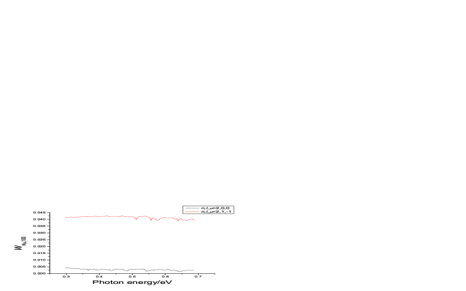
Figure 1: Transition probabilities of a hydrogen atom interacting with a circularly polarized laser of $A=5\times 10^{-6}$V$\cdot$s/m, and their dependence on the photon energy.

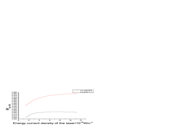
Figure 2: Transition probabilities of a hydrogen atom interacting with a circularly polarized laser of $\hbar\omega=0.296$eV, and their dependence on the laser intensity.

Fig.1 shows that the spectrum is continuous. No discrete sharp resonance peaks appear. If one fits the spectrum by (3), $\eta$ may take any real number in a wide range, not necessarily be an integer. The transition is non-integer. While fig.2 shows that the transition probability is not proportional to an integer power of the laser intensity. It means, the interaction between the laser and the atom cannot be reduced to the interaction of individual photons with the atom separately. The interaction is between the atom and the laser as a whole. This scenery is quite different from the regularity one saw in the weak light (including weak laser) spectroscopy, therefore has to be checked by new experiments. One may observe the radiation of the atom when it is irradiated by an intense laser. This is the laser Raman effect. In this way, the changes of distributions of atoms among various energy levels, and therefore their transition probabilities, are measured. Although there is not any separate resonance, fig.1 still shows complex structure in the spectrum. It is interesting to find out the information exposed by this kind of structure.

3 Laser photo-ionizations

The photo-ionization or the photoelectric effect is the transition of the electron from the ground state to the ionized state, when it is irradiated by light. The photo-ionization by an intense circularly polarized laser may be handled by the method proposed in [4]. Some preliminary results obtained by this method have been reported in [4]-[6]. Here we would analyze it from the view point of non-integer quantum transition.

It is shown in [4], that the energy of the ionized electron (photo-electron) is

$$E_{f0}=E_{i}-\mu\hbar\omega\ ,$$ (27)

and the transition probability per unit time is

$$P=\frac{2\pi}{\hbar}\left|H_{f0,i}^{\prime\prime}\right|^{2}\rho\ ,$$ (28)

with

$$H_{f0,i}^{\prime\prime}\equiv\int\psi_{f0}({\textit{{r}}})\hat{H}^{\prime\prime}\phi_{i}({\textit{{r}}}){\rm d}{\textit{{r}}}\ .$$ (29)

$\phi_{i}({\textit{{r}}})$ in (29) is an eigenfunction of $\hat{H}_{\rm ps}$, satisfying (14). $E_{i}$ in (27) is the corresponding eigenvalue. $\psi_{f0}({\textit{{r}}})$ is the eigenfunction of $\hat{H}_{0}^{\prime}$, with eigenvalue $E_{f0}+\mu\hbar\omega$, therefore is a projection of the Coulomb wave function onto the subspace with definite magnetic quantum number $\mu$, and describes the ionized electron.

In the weak light limit, $A\rightarrow 0$, $\phi_{i}$ approaches an eigenfunction of $\hat{H}_{0}^{\prime}$, which is also the ground state eigenfunction of $\hat{H}_{0}$ with zero magnetic quantum number; and $E_{i}$ approaches the corresponding eigenvalue. They are independent of $A$. For the hydrogen atom, they are $\psi_{100}$ and $-b$ respectively, $b$ is the binding energy of the electron in the ground state hydrogen atom. In the case of $ka_{0}<<1$, we have (24), therefore the selection rule (25) works. These limits make the energy (27) of the photoelectron be

$$E_{f0}=\hbar\omega-b\ ,$$ (30)

and the transition probability $P$ proportional to the light intensity. This example shows, in the weak light limit, the photo-ionization has the following distinct characters:

C1.There is a critical frequency for a given system.The light with frequency lower than this critical value cannot eject any electron from the system.

C2.The light with frequency higher than this critical value can ionize the system, the energy of the ejected electron increases linearly with the increasing of the frequency but is independent of the intensity of the light.

C3.The intensity of the photo-electric current is proportional to the intensity of the light.

This is exactly the experimental knowledge on photo-ionization, people had before the discovery of the laser. Based on this knowledge and guided by his idea of light quanta, one hundred years ago, Einstein [7] found his famous formula (30) and the idea that the light-atom interaction may be reduced to the interactions between photons and atoms. In this way, he explained the above experimental characters of photo-ionization. This was a crucial step towards the discovery of quantum mechanics. Now we see, all of these experimental characters, as well as the Einstein formula (30), together with his idea that photons interact with atoms independently, are the perturbation results of quantum mechanics in the weak light limit. What will be the scenery when the light becomes an intense laser?

If one puts $E_{1}=-b$ , and $E_{2}=E_{f0}$, the formula (30) becomes (1) with the positive sign on the right. Therefore, the Einstein formula is a predecessor of the Bohr condition. Soon after the discovery of laser, people observed the MPI[1] and the ATI[2]. Einstein formula was generalized to be

$$E_{f0}=N\hbar\omega-b\ ,$$ (31)

with $N$ being an positive integer. This is something like a special case of the generalized Bohr condition (2) and may be deduced by the higher order perturbation. (27) would be an exact expression of the photoelectron energy, if $E_{i}$ in it is solved from (14) exactly. Defining

$$\eta\equiv\frac{E_{i}+b}{\hbar\omega}-\mu\ ,$$ (32)

one may write (27) in the form

$$E_{f0}=\eta\hbar\omega-b\ .$$ (33)

It is a special case of (3). Here we see, $\eta$ is an integer only when $E_{i}+b-\mu\hbar\omega$ is an integer multiple of the photon energy $\hbar\omega$. This will not necessarily be the case for a non-perturbation interaction between the atom and an intense laser. It means the photo-ionization will be a non-integer quantum transition. This is the true non-perturbation effect. Using the numerical solution of (14) obtained in the last section, we find the light intensity dependence of the photoelectron energy. The numerical result is shown in fig.3.

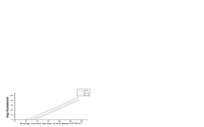
Figure 3: The energy of a photoelectron ejected from the ground state hydrogen atom by a circularly polarized laser of $\hbar\omega=2.37$eV, and its dependence on the laser intensity.

The transition probability (28) may be expressed in the form of cross section. It is the formula (14) or (15) in [4]. Applying it to the photo-ionization of the hydrogen atom irradiated by a circularly polarized laser, under the condition $ka_{0}<<1$, we obtain the cross section

$$\sigma=\frac{16\alpha v}{ka_{0}c}\sum_{l=|\mu|}\left|\beta_{l}(i)\right|^{2}$$ (34)

in unit of $\pi a_{0}^{2}$. Here, $v=\sqrt{2E_{f0}/m}$ is the velocity of the photoelectron, and $\beta_{l}(i)$ is an elementary but some what lengthy and tedious expression, containing integrals of the type

$$\int_{0}^{\infty}{\rm e}^{-st}t^{u-1}{\rm F}(a_{1},c_{1},t){\rm F}(a_{2},c_{2},qt){\rm d}t=\Gamma(u)s^{-u}{\rm F}_{2}(u,a_{1},a_{2},c_{1},c_{2},s^{-1},\frac{q}{s})\ .$$ (35)

The integral has been analytically worked out. There are two confluent hypergeometric functions F on the left. One is from the radial wave function of the electron in the hydrogen atom, and another is from the Coulomb wave function of the outgoing electron. ${\rm F}_{2}$ on the right is the Appell’s hypergeometric function of the second class in two variables[8]. In our problem here, it degenerates into a polynomial in two variables. Therefore the calculation of $\beta_{l}(i)$ becomes finite, if the expansion (16) is truncated. The calculated cross section and its dependence on the laser intensity is shown in fig.4.

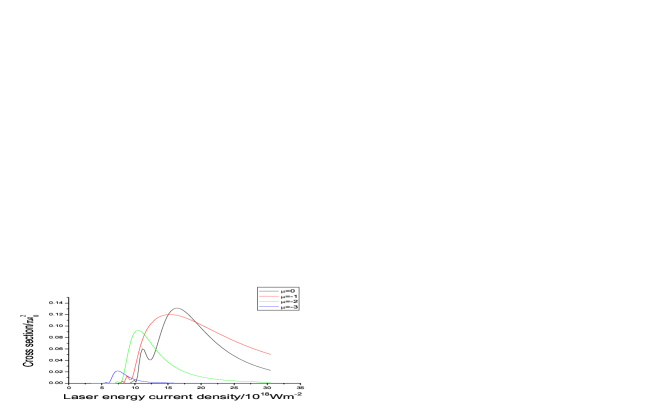
Figure 4: Cross section of the photo-ionization of a ground state hydrogen atom irradiated by a circularly polarized laser of $\hbar\omega=2.37$eV, and its dependence on laser intensity.

We see from fig.3, the energy of the photo-electron increases with the increasing of the light intensity. The critical frequency is not absolute. Even though the frequency of the incident light is lower than the critical frequency, the electron may still be ejected, if the light is intense enough. The characters C2 and C1, together with the formula (30), are not true for laser photo-ionization. Furthermore, the formula (31) is not true either, if the incident laser is very strong. In this case, it has to be substituted by (33), with non-integer $\eta$. The transition in photo-ionization becomes non-integer. However, one may still see an apparent quantum character in fig.3. That is, the energy difference between photo-electrons with different magnetic quantum number $\mu$ is an integer multiple of the quantum energy $\hbar\omega$. From fig.4 we see, the cross sections depend on the light intensity nonlinearly. It means that the character C3 is not true for laser photo-ionization. The interaction between light and atoms cannot be reduced to the independent interactions between photons and atoms. Atoms interact with the laser as a whole.

4 Omitted effects

We omitted some effects in the foregoing sections. Here let us say a few words on them.

4.1 The motion of the nucleus

The hydrogen atom consists of a proton and an electron. To consider the motion of the proton, one has to change (7) into

$$\hat{H}_{0}=\frac{\hat{p}_{1}^{2}}{2m_{1}}+\frac{\hat{p}_{2}^{2}}{2m_{2}}+V(r)\ ,$$ (36)

and (8) into

$$\hat{H}^{\prime} = \frac{eA}{m_{1}}[\hat{p}_{1x}\cos(kz_{1}-\omega t)+\hat{p}_{1y}\sin(kz_{1}-\omega t)]+\frac{e^{2}A^{2}}{2m_{1}}$$ (37)

$$- \frac{eA}{m_{2}}[\hat{p}_{2x}\cos(kz_{2}-\omega t)+\hat{p}_{2y}\sin(kz_{2}-\omega t)]+\frac{e^{2}A^{2}}{2m_{2}}\ .$$

Subscripts 1 and 2 denote the electron and the proton respectively. Substituting them into (6) and (9), and performing the transformation

$$\Psi({\textit{{r}}}_{1},{\textit{{r}}}_{2},t)={\rm e}^{{\rm i}\omega(\hat{L}_{1z}+\hat{L}_{2z})t/\hbar}\Phi({\textit{{r}}}_{1}{\textit{{r}}}_{2},t)\ ,$$ (38)

one obtains again the time independent pseudo-Schrödinger equation (11). But now one has to substitute

$$\hat{H}_{0}^{\prime}=\hat{H}_{0}+\omega\sum_{j=1}^{2}\hat{L}_{jz}$$ (39)

and

$$\hat{H}^{\prime\prime} = \frac{eA}{m_{1}}[\hat{p}_{1x}\cos(kz_{1})+\hat{p}_{1y}\sin(kz_{1})]+\frac{e^{2}A^{2}}{2m_{1}}$$ (40)

$$- \frac{eA}{m_{2}}[\hat{p}_{2x}\cos(kz_{2})+\hat{p}_{2y}\sin(kz_{2})]+\frac{e^{2}A^{2}}{2m_{2}}$$

into the pseudo-Hamiltonian (12). A further transformation

$$\Phi=\exp\left[-{\rm i}k\frac{(m_{1}z_{1}+m_{2}z_{2})(\hat{L}_{1z}+\hat{L}_{2z})}{(m_{1}+m_{2})\hbar}\right]\Phi_{\rm e}$$ (41)

brings (11) to

$${\rm i}\hbar\frac{\partial\Phi_{\rm e}}{\partial t}=\hat{H}_{\rm e}\Phi_{\rm e}\ ,$$ (42)

with the effective Hamiltonian

$$\hat{H}_{\rm e} = \sum_{j=1}^{2}\left[\frac{\hat{p}_{jx}^{2}+\hat{p}_{jy}^{2}+(\hat{p}_{jz}-m_{j}k\frac{\hat{L}_{1z}+\hat{L}_{2z}}{m_{1}+m_{2}})^{2}}{2m_{j}}+\omega\hat{L}_{jz}\right]+V(r)$$ (43)

$$+ \frac{eA}{m_{1}}\left[\hat{p}_{1x}\cos\left(km_{2}\frac{z_{1}-z_{2}}{m_{1}+m_{2}}\right)+\hat{p}_{1y}\sin\left(km_{2}\frac{z_{1}-z_{2}}{m_{1}+m_{2}}\right)\right]+\frac{e^{2}A^{2}}{2m_{1}}$$

$$- \frac{eA}{m_{2}}\left[\hat{p}_{2x}\cos\left(km_{1}\frac{z_{2}-z_{1}}{m_{1}+m_{2}}\right)+\hat{p}_{2y}\sin\left(km_{1}\frac{z_{2}-z_{1}}{m_{1}+m_{2}}\right)\right]+\frac{e^{2}A^{2}}{2m_{2}}\ .$$

Introducing the center of mass coordinates ${\textit{{R}}}\equiv(m_{1}{\textit{{r}}}_{1}+m_{2}{\textit{{r}}}_{2})/M$ and the relative coordinates ${\textit{{r}}}\equiv{\textit{{r}}}_{1}-{\textit{{r}}}_{2}$, we have the total momentum $\hat{\textit{{P}}}=\hat{\textit{{p}}}_{1}+\hat{\textit{{p}}}_{2}$, the relative momentum $\hat{\textit{{p}}}=m(\hat{\textit{{p}}}_{1}/m_{1}-\hat{\textit{{p}}}_{2}/m_{2})$, the angular momentum $\hat{\textit{{L}}}_{c}={\textit{{R}}}\times\hat{\textit{{P}}}$ of the center of mass, and the angular momentum $\hat{\textit{{L}}}={\textit{{r}}}\times\hat{\textit{{p}}}$ around the center of mass. $M=m_{1}+m_{2}$ is the total mass, and $m=m_{1}m_{2}/(m_{1}+m_{2})$ is the reduced mass. In these coordinates, the effective Hamiltonian (43) has the form

$$\hat{H}_{\rm e} = \frac{\hat{\textit{{P}}}_{x}^{2}+\hat{\textit{{P}}}_{y}^{2}+[\hat{\textit{{P}}}_{z}-k(\hat{L}_{cz}+\hat{L}_{z})]^{2}}{2M}+\omega\hat{L}_{cz}$$ (44)

$$+ \frac{p^{2}}{2m}+V(r)+\omega\hat{L}_{z}+\frac{eA}{m}\hat{p}_{x}+\frac{e^{2}A^{2}}{2m}\ ,$$

at the limit of $ka_{0}\rightarrow 0$. The sum of the last five terms relates to the relative motion only, and equals the pseudo-Hamiltonian (12) (together with (13)) at the same limit of $ka_{0}\rightarrow 0$, if $m$ there is also understood to be the reduced mass instead of the electron mass. The first two terms mainly relate to the motion of the center of mass. Only $\hat{L}_{z}$ in the first term relates to the relative motion. But the big mass $M$ on the denominator makes its contribution be much less than that of the last five terms. Therefore, one needs only to consider the sum of the last five terms in (44), for the problem of relative motion between the electron and the proton in hydrogen atom, irradiated by a circularly polarized laser. The correction of the nucleus motion is again the substitution of the reduced mass for the electron mass. It is tiny. The first two terms in (44) govern the motion of the hydrogen atom as a whole. They have to be considered if one is interested in the motion of ionized electrons, for example, their angular distributions.

4.2 The quantization of the electromagnetic field

In a complete theory, the electromagnetic field has to be quantized. In the Coulomb gauge, it is to let the vector potential be an operator $\hat{\textit{{A}}}$ and define commutators between its components. Introducing a complete set of vector functions $[{\textit{{A}}}_{\iota}({\textit{{r}}})]$, satisfying the Helmholtz equations

$$\nabla^{2}{\textit{{A}}}_{\iota}({\textit{{r}}})+\frac{\omega_{\iota}^{2}}{c^{2}}{\textit{{A}}}_{\iota}({\textit{{r}}})=0$$ (45)

and the orthonomal conditions

$$\int{\textit{{A}}}_{\iota}^{*}({\textit{{r}}})\cdot{\textit{{A}}}_{\iota}^{\prime}({\textit{{r}}}){\rm d}{\textit{{r}}}=\delta_{\iota\iota^{\prime}}\ ,$$ (46)

one may expand the self-adjoint operator

$$\hat{\textit{{A}}}({\textit{{r}}},t)=\sum_{\iota}\sqrt{\frac{\hbar}{2\epsilon_{0}\omega_{\iota}}}\left[\hat{b}_{\iota}{\textit{{A}}}_{\iota}({\textit{{r}}})+\hat{b}_{\iota}^{\dagger}{\textit{{A}}}_{\iota}^{*}({\textit{{r}}})\right]\ ,$$ (47)

$\epsilon_{0}$ is the dielectric constant for the vacuum. The quantization condition is the commutators

$$\hat{b}_{\iota}\hat{b}_{\iota^{\prime}}-\hat{b}_{\iota^{\prime}}\hat{b}_{\iota}=\hat{b}_{\iota}^{\dagger}\hat{b}_{\iota^{\prime}}^{\dagger}-\hat{b}_{\iota^{\prime}}^{\dagger}\hat{b}_{\iota}^{\dagger}=0\ ,\;\;\;\;\mbox{and}\;\;\;\;\hat{b}_{\iota}\hat{b}_{\iota^{\prime}}^{\dagger}-\hat{b}_{\iota^{\prime}}^{\dagger}\hat{b}_{\iota}=\delta_{\iota\iota^{\prime}}\ .$$ (48)

The vacuum state $|0\rangle$ is defined by

$$\hat{b}_{\iota}|0\rangle=0\;\;\;\;\;\;\mbox{for all $\iota$}\ .$$ (49)

This is the quantization around the vacuum. Classically, the vacuum is described by a vector potential ${\textit{{A}}}_{0}({\textit{{r}}},t)=0$, which is a trivial solution of the D’Alembert equation. It suggests, that one may also quantize the theory around another classical solution ${\textit{{A}}}_{c}({\textit{{r}}},t)$, for example the solution (5), of the D’Alembert equation. Defining $\hat{\textit{{A}}}^{\prime}({\textit{{r}}},t)=\hat{\textit{{A}}}({\textit{{r}}},t)-{\textit{{A}}}_{c}({\textit{{r}}},t)$, expanding

$${\textit{{A}}}_{c}({\textit{{r}}},t)=\sum_{\iota}\sqrt{\frac{\hbar}{2\epsilon_{0}\omega_{\iota}}}\left[c_{\iota}{\textit{{A}}}_{\iota}({\textit{{r}}})+c_{\iota}^{*}{\textit{{A}}}_{\iota}^{*}({\textit{{r}}})\right]\ ,$$ (50)

we have

$$\hat{\textit{{A}}}^{\prime}({\textit{{r}}},t)=\sum_{\iota}\sqrt{\frac{\hbar}{2\epsilon_{0}\omega_{\iota}}}\left[\hat{b}_{\iota}^{\prime}{\textit{{A}}}_{\iota}({\textit{{r}}})+\hat{b}_{\iota}^{\prime{\dagger}}{\textit{{A}}}_{\iota}^{*}({\textit{{r}}})\right]\ ,$$ (51)

with

$$\hat{b}^{\prime}_{\iota}=\hat{b}_{\iota}-c_{\iota}\ .$$ (52)

Since $c_{\iota}$ are c-numbers, $\hat{b}_{\iota}^{\prime}$ and $\hat{b}_{\iota}^{\prime{\dagger}}$ have the same commutators as those for $\hat{b}_{\iota}$ and $\hat{b}_{\iota}^{\dagger}$. They are

$$\hat{b}_{\iota}^{\prime}\hat{b}_{\iota^{\prime}}^{\prime}-\hat{b}_{\iota^{\prime}}^{\prime}\hat{b}_{\iota}^{\prime}=\hat{b}_{\iota}^{\prime{\dagger}}\hat{b}_{\iota^{\prime}}^{\prime{\dagger}}-\hat{b}_{\iota^{\prime}}^{\prime{\dagger}}\hat{b}_{\iota}^{\prime{\dagger}}=0\ ,\;\;\;\;\mbox{and}\;\;\;\;\hat{b}_{\iota}^{\prime}\hat{b}_{\iota^{\prime}}^{\prime{\dagger}}-\hat{b}_{\iota^{\prime}}^{\prime{\dagger}}\hat{b}_{\iota}^{\prime}=\delta_{\iota\iota^{\prime}}\ .$$ (53)

The quantization condition for the electromagnetic field $\hat{\textit{{A}}}^{\prime}$ around a classical field ${\textit{{A}}}_{c}$ is therefore the same as that for the field $\hat{\textit{{A}}}$ around the classical vacuum ${\textit{{A}}}_{0}=0$. However, the ’vacuum’ state is now changed to $|c\rangle$, satisfying $\hat{b}_{\iota}^{\prime}|c\rangle=0$. This is

$$\hat{b}_{\iota}|c\rangle=c_{\iota}|c\rangle\ ,$$ (54)

showing that $|c\rangle$ is a coherent state with non-zero amplitude(s) $c_{\iota}$. In the classical limit it is ${\textit{{A}}}_{c}$ itself.

The interaction operator between the electromagnetic field and a non-relativistic electron is

$$\frac{e}{m}\hat{\textit{{A}}}\cdot\hat{\textit{{p}}}+\frac{e^{2}\hat{\textit{{A}}}^{2}}{2m}=\frac{e}{m}{\textit{{A}}}_{c}\cdot\hat{\textit{{p}}}+\frac{e^{2}A_{c}^{2}}{2m}+\frac{e}{m}\hat{\textit{{A}}}^{\prime}\cdot\hat{\textit{{p}}}+\frac{e^{2}\hat{\textit{{A}}}^{\prime 2}}{2m}+\frac{e^{2}\hat{\textit{{A}}}^{\prime}\cdot{\textit{{A}}}_{c}}{m}\ .$$ (55)

If ${\textit{{A}}}_{c}$ represents an intense laser, the first two terms on the right would be large, its effect has to be treated non-perturbatively. It is the main part of the problem. This is what we have done in the above sections. For a few fluctuations of the electromagnetic field around the laser, the remaining terms on the right of this equation are small, and may be considered by perturbation, if it is needed.

4.3 The relativity and spin effects of the electron

The method used above may be applied to a relativistic particle system with spin as well. The way is to use the total angular momentum $\hat{\textit{{J}}}$, instead of the orbital angular momentum $\hat{\textit{{L}}}$, in the transformation (10). In this way, the transformation reads

$$\Psi={\rm e}^{{\rm i}\omega\hat{J}_{z}t/\hbar}\Phi\ .$$ (56)

The relativity is not important in most problems. One can easily consider the electron spin by applying this transformation in solving the Pauli equation for electrons in an atom, irradiated by the circularly polarized laser, whenever he is interested in the problem of electron polarization in the process.

5 Conclusion

We see, a laser may not only induce MPI and ATI, but also cause non-integer transitions, if it is strong enough. The later can only be handled by non-perturbation method, and therefore is a non-perturbation effect.

One hundred years ago, people knew very few about the photo-electric effects. There was not a laser. People could see the effect only when irradiating matter by usual light. It is very weak from the present view point. But, just under this condition, the distinct characters C1-C3 shown in section 3 appear. It was these distinct characters made Einstein find the light quanta by his keen insight, which was one of the important steps towards the discovery of quantum mechanics. Several decades later, people predicted and constructed the laser by the guide of quantum mechanics. Now we see, again by the guide of quantum mechanics, if one irradiates matter by intense laser, very fruitful and complex phenomena will appear, and those distinct characters disappear. We are fortunate, that people discovered usual light instead of the laser first, so that Einstein could see the distinct characters and discover the light quanta one hundred years ago. We learn from this history, that sometimes simple experimental phenomena may expose essentials; on the contrary, too fruitful experimental data may conceal essential points. In any case, a keen insight is always important.

References

• [1] G.S. Voronov and N.B. Delone ,Sov. Phys. JETP 23 (1966) 54
• [2] P. Agostini, F. Fabre, G. Mainfray, G. Petite and N.K. Rahman, Phys.Rev.Lett. 42, (1979) 1127
• [3] J.H. Wilkinson The Algebraic Eigenvalue Problem, Clarendon Press, Oxford, 1965
• [4] Qi-Ren Zhang , Physics Letters A 216 (1996) 125
• [5] Deng Zhang and Qi-Ren Zhang, Comm. Theor. Phys. 36 (2001) 685
• [6] Xiang-Tao Liu, Qi-Ren Zhang, and Wan-Zhang Wang, Comm. Theor. Phys. 41 (2004) 461
• [7] A. Einstein Ann. Phys. (Leipzig) 17 (1905) 132
• [8] A. Erd$\acute{e}$lyi Higher Transcendental Functions I, McGraw Hill, New York, 1953