Nonlocality without inequality for almost all two-qubit entangled state based on Cabello’s nonlocality argument

Here we deal with a nonlocality argument proposed by Cabello which is more general than Hardy’s nonlocality argument but still maximally entangled states do not respond. However, for most of the other entangled states maximum probability of success of this argument is more than that of the Hardy’s argument.

Introduction

It is well known result that realistic interpretations of quantum theory are nonlocal [1]. This was first shown by means of Bell’s inequality. Afterwards, the proof of the same for three spin-1/2 particles as well as for two spin-1 particles, without using inequality caused much interest among physicists [2]. Surprisingly Hardy gave a proof of nonlocality without using inequality, for two spin-1/2 particles which requires two measurement settings on both the sides as happens in case of Bell’s argument [3]. Later Hardy showed this kind of nonlocality argument can be made for almost all entangled state of two spin-1/2 particles except for maximally entangled one.[4]. He considered the cases where the measurement choices were same for both the parties. Jordan showed that for any given entangled state of two spin-1/2 particles except maximally entangled state there are many set of observables on each side which satisfy Hardy’s nonlocality conditions [5]. Jordan also showed that the set of observables which gives maximum probability of success in showing the contradiction with local-realism, is the same as chosen by Hardy.
Recently Cabello has introduced a logical structure to prove Bell’s theorem without inequality for three particles GHZ and W state [6]. Logical structure presented by Cabello is as follows : Consider four events D, E, F and G where D and F may happen in one system and E and G happen in another system which is far apart from the first. The probability of joint occurrence of D and E is non-zero, E always implies F, D always implies G, but F and G happen with lower probability than D and E. These four statements are not compatible with local realism. The difference between these two probabilities is the measure of violation of local realism. Though Cabello’s logical structure was originally proposed for showing nonlocality for three particle states but Liang and Li [7] exploited it in establishing nonlocality without inequality for a class of two qubit mixed entangled state. In this sense, Hardy’s logical structure is an special case of Cabello’s structure as the logical structure of Hardy for establishing nonlocality is as follows: D and E sometimes happen, E always implies F, D always implies G, but F and G never happen. Recently based on Cabello’s logical structure Kunkri and Choudhary [8] have shown that there may be many classes of two qubit mixed states which exhibit nonlocality without inequality. It is noteworthy here that in contrast there is no two qubit mixed state which shows Hardy type nonlocality [9]. So it seems interesting to study that whether maximally entangled states follow this more general (than Hardy’s), Cabello’s nonlocality argument or not , because Hardy’s nonlocality argument is not followed by a maximally entangled state. In this paper we have studied it and found that maximally entangled states do not respond even to this argument. However, for all other pure entangled states , Cabello’s argument runs. We further have enquired about the highest value of difference between the two probabilities which appear in Cabello’s argument. Surprisingly this value differs from the highest value of probability which appears in Hardy’s argument.

Cabello’s argument for two qubits

Let us consider two spin-1/2 particles A and B. Let F, D, G and E represent the spin observables along $n_{F}(\sin{\theta_{F}}\cos{\phi_{F}},\sin{\theta_{F}}\sin{\phi_{F}},\cos{\theta_{F}})$, $n_{D}(\sin{\theta_{D}}\cos{\phi_{D}},\sin{\theta_{D}}\sin{\phi_{D}},\cos{\theta_{D}})$, $n_{G}(\sin{\theta_{G}}\cos{\phi_{G}},\sin{\theta_{G}}\sin{\phi_{G}},\cos{\theta_{G}})$ and $n_{E}(\sin{\theta_{E}}\cos{\phi_{E}},\sin{\theta_{E}}\sin{\phi_{E}},\cos{\theta_{E}})$ respectively. Every observable has the eigen value $\pm 1$. Let F and D are measured on particle A and G and E are measured on particle B. Now we consider the following equations

$$P(F=+1,G=+1)=q_{1}$$ (1)

$$P(D=+1,G=-1)=0$$ (2)

$$P(F=-1,E=+1)=0$$ (3)

$$P(D=+1,E=+1)=q_{4}$$ (4)

Equation (1) tells that if F is measured on particle A and G is measured on particle B, then the probability that both will get +1 eigen value is $q_{1}$. Other equations can be analyzed in a similar fashion. These equations form the basis of Cabello’s nonlocality argument. It can easily be seen that these equations contradict local-realism if $q_{1}<q_{4}$. To show this, let us consider those hidden variable states $\lambda$ for which $D=+1$ and $E=+1$. Now for these states equations $(2)$ and $(3)$ tell that the values of $G$ and $F$ must be equal to $+1$. Thus according to local realism $P(F=+1,G=+1)$ should be at least equal to $q_{4}$, which contradicts equation $(1)$ as $q_{1}<q_{4}$. It should be noted here that $q_{1}=0$ reduces this argument to Hardy’s one. So by Cabello’s argument we specifically mean that the above argument runs even with nonzero $q_{1}$.
Now we will show that for almost all two qubit pure entangled state other than maximally entangled one this kind of nonlocality argument runs. Following Schmidt decomposition procedure any entangled state of two particles A and B can be written as

$$|\psi\rangle=(\cos{\beta})|0\rangle_{A}|0\rangle_{B}+(\sin{\beta})e^{i\gamma}|1\rangle_{A}|1\rangle_{B}$$ (5)

If either $\cos{\beta}$ or $\sin{\beta}$ is zero, we have a product state not an entangled state. Then it is not possible to satisfy equation $(1)-(4)$. Hence we assume that neither $\cos{\beta}$ nor $\sin{\beta}$ is zero; both are positive.
The density matrix for the above state is

$$\begin{array}[]{lcl}\rho=\frac{1}{4}[I^{A}\otimes I^{B}+(\cos^{2}{\beta}-\sin^{2}{\beta})I^{A}\otimes\sigma_{z}^{B}+(\cos^{2}{\beta}-\sin^{2}{\beta})\sigma_{z}^{A}\otimes I^{B}\\ +(2\cos{\beta}\sin{\beta}\cos{\gamma})\sigma_{x}^{A}\otimes\sigma_{x}^{B}+(2\cos{\beta}\sin{\beta}\sin{\gamma})\sigma_{x}^{A}\otimes\sigma_{y}^{B}\\ +(2\cos{\beta}\sin{\beta}\sin{\gamma})\sigma_{y}^{A}\otimes\sigma_{x}^{B}-(2\cos{\beta}\sin{\beta}\cos{\gamma})\sigma_{y}^{A}\otimes\sigma_{y}^{B}+\sigma_{z}^{A}\otimes\sigma_{z}^{B}]\end{array}$$ (6)

Where $\sigma_{x}$, $\sigma_{y}$ and $\sigma_{z}$ are Pauli operators. Now for this state if F is measured on particle A and G is measured on particle B, then the probability that both will get +1 eigen value is given by

$$\begin{array}[]{lcl}P(F=+1,G=+1)=(\frac{1}{4})[1+(\cos^{2}{\beta}-\sin^{2}{\beta})(\cos{\theta_{F}}+\cos{\theta_{G}})\\ +\cos{\theta_{F}}\cos{\theta_{G}}+2\cos{\beta}\sin{\beta}\sin{\theta_{F}}\sin{\theta_{G}}\times\cos{(\phi_{F}+\phi_{G}-\gamma)}]\end{array}$$ (7)

Rearranging the above expression we get

$$\begin{array}[]{lcl}P(F=+1,G=+1)=\cos^{2}{\beta}\cos^{2}{\frac{\theta_{F}}{2}}\cos^{2}{\frac{\theta_{G}}{2}}+\sin^{2}{\beta}\sin^{2}{\frac{\theta_{F}}{2}}\sin^{2}{\frac{\theta_{G}}{2}}+\\ +2\cos{\beta}\sin{\beta}\cos{\frac{\theta_{F}}{2}}\sin{\frac{\theta_{F}}{2}}\cos{\frac{\theta_{G}}{2}}\sin{\frac{\theta_{G}}{2}}\times\cos{(\phi_{F}+\phi_{G}-\gamma)}]=q_{1}(say)\end{array}$$ (8)

Similar calculations for other probabilities give us:

$$\begin{array}[]{lcl}P(D=+1,G=-1)=\cos^{2}{\beta}\cos^{2}{\frac{\theta_{D}}{2}}\sin^{2}{\frac{\theta_{G}}{2}}+\sin^{2}{\beta}\sin^{2}{\frac{\theta_{D}}{2}}\cos^{2}{\frac{\theta_{G}}{2}}+\\ +2\cos{\beta}\sin{\beta}\cos{\frac{\theta_{D}}{2}}\sin{\frac{\theta_{D}}{2}}\cos{\frac{\theta_{G}}{2}}\sin{\frac{\theta_{G}}{2}}\times\cos{(\phi_{D}+\phi_{G}+\pi-\gamma)}]=q_{2}(say)\end{array}$$ (9)

$$\begin{array}[]{lcl}P(F=-1,E=+1)=\cos^{2}{\beta}\cos^{2}{\frac{\theta_{E}}{2}}\sin^{2}{\frac{\theta_{F}}{2}}+\sin^{2}{\beta}\sin^{2}{\frac{\theta_{E}}{2}}\cos^{2}{\frac{\theta_{F}}{2}}+\\ +2\cos{\beta}\sin{\beta}\cos{\frac{\theta_{F}}{2}}\sin{\frac{\theta_{F}}{2}}\cos{\frac{\theta_{E}}{2}}\sin{\frac{\theta_{E}}{2}}\times\cos{(\phi_{F}+\phi_{E}+\pi-\gamma)}]=q_{3}(say)\end{array}$$ (10)

$$\begin{array}[]{lcl}P(D=+1,E=+1)=\cos^{2}{\beta}\cos^{2}{\frac{\theta_{D}}{2}}\cos^{2}{\frac{\theta_{E}}{2}}+\sin^{2}{\beta}\sin^{2}{\frac{\theta_{D}}{2}}\sin^{2}{\frac{\theta_{E}}{2}}+\\ +2\cos{\beta}\sin{\beta}\cos{\frac{\theta_{D}}{2}}\sin{\frac{\theta_{D}}{2}}\cos{\frac{\theta_{E}}{2}}\sin{\frac{\theta_{E}}{2}}\times\cos{(\phi_{D}+\phi_{E}-\gamma)}]=q_{4}(say)\end{array}$$ (11)

For running Cabello’s nonlocality argument, following conditions should be satisfied:

$$q_{2}=0,~{}~{}q_{3}=0,~{}~{}(q_{4}-q_{1})>0,~{}~{}q_{1}>0$$ (12)

Since $q_{2}$ represents probability, it can not be negative. If it is zero, it is at its minimum value. Then its derivative must be zero. From it’s derivative with respect to $\phi_{D}$ we see that $\sin{(\phi_{D}+\phi_{G}+\pi-\gamma)}$ must be zero. Evidently

$$\cos{(\phi_{D}+\phi_{G}+\pi-\gamma)}=-1$$ (13)

We conclude that if $q_{2}$ is zero, then

$$\cos{\beta}\cos{\frac{\theta_{D}}{2}}\sin{\frac{\theta_{G}}{2}}=\sin{\beta}\sin{\frac{\theta_{D}}{2}}\cos{\frac{\theta_{G}}{2}}$$ (14)

Similar sort of argument for $q_{3}$ to be zero will give:

$$\cos{(\phi_{F}+\phi_{E}+\pi-\gamma)}=-1$$ (15)

and

$$\cos{\beta}\cos{\frac{\theta_{E}}{2}}\sin{\frac{\theta_{F}}{2}}=\sin{\beta}\sin{\frac{\theta_{E}}{2}}\cos{\frac{\theta_{F}}{2}}$$ (16)

Maximally entangled states of two spin-1/2 particles do not exhibit Cabello type nonlocality-

For maximally entangled state $\tan{\beta}=1$, then from equations $(14)$ and $(16)$ we get

$$\frac{\theta_{G}}{2}=\frac{\theta_{D}}{2}+n\pi$$ (17)

$$\frac{\theta_{F}}{2}=\frac{\theta_{E}}{2}+m\pi$$ (18)

Using equations $(17)$ and $(18)$ first in equation $(8)$ and then in equation (11) we get $q_{1}$ and $q_{4}$ for maximally entangled state as:

$$\begin{array}[]{lcl}q_{1}=\frac{1}{2}\cos^{2}{\frac{\theta_{D}}{2}}\cos^{2}{\frac{\theta_{E}}{2}}+\frac{1}{2}\sin^{2}{\frac{\theta_{D}}{2}}\sin^{2}{\frac{\theta_{E}}{2}}\\ +\cos{\frac{\theta_{D}}{2}}\sin{\frac{\theta_{D}}{2}}\cos{\frac{\theta_{E}}{2}}\sin{\frac{\theta_{E}}{2}}\times\cos{(\phi_{F}+\phi_{G}-\gamma)}]\end{array}$$ (19)

$$\begin{array}[]{lcl}q_{4}=\frac{1}{2}\cos^{2}{\frac{\theta_{D}}{2}}\cos^{2}{\frac{\theta_{E}}{2}}+\frac{1}{2}\sin^{2}{\frac{\theta_{D}}{2}}\sin^{2}{\frac{\theta_{E}}{2}}\\ +\cos{\frac{\theta_{D}}{2}}\sin{\frac{\theta_{D}}{2}}\cos{\frac{\theta_{E}}{2}}\sin{\frac{\theta_{E}}{2}}\times\cos{(\phi_{D}+\phi_{E}-\gamma)}]\end{array}$$ (20)

From equations $(19)$ and $(20)$ it is clear that $q_{4}$ will be grater than $q_{1}$ for a maximally entangled state only when $\cos{(\phi_{D}+\phi_{E}-\gamma)}>\cos{(\phi_{F}+\phi_{G}-\gamma)}$. But equation $(13)$ together with equation $(15)$ says that $\cos{(\phi_{D}+\phi_{E}-\gamma)}=\cos{(\phi_{F}+\phi_{G}-\gamma)}$ i.e $q_{4}=q_{1}$. So one can conclude that there is no choice of observable which can make maximally entangled state to show Cabello type of nonlocality .

Cabello’s argument runs for other two particle pure entangled states-

To show that for every pure entangled state other than maximally entangled state of two spin-1/2 particles, Cabello like argument runs it will be sufficient to show that one can always choose a set of observables for which set of conditions given by equation (12) is satisfied. This is equivalent of saying that for $0<\beta<\frac{\pi}{2}$ except when $\beta=\frac{\pi}{4}$ there is at least one value for each of $\theta_{D}$,$\theta_{E}$,$\theta_{G}$,$\theta_{F},\phi_{D}$,$\phi_{E}$,$\phi_{G}$,$\phi_{F}$ for which conditions mentioned in(12) are satisfied.
Let us choose our $\phi^{\prime}s$ in such a manner that

$$cos{(\phi_{F}+\phi_{G}-\gamma)}=cos{(\phi_{D}+\phi_{E}-\gamma)}=-1$$

For these $\phi^{\prime}s$ equations (8) and (11) respectively will read as:

$$q_{1}=(\cos{\beta}\cos{\frac{\theta_{F}}{2}}\cos{\frac{\theta_{G}}{2}}-\sin{\beta}\sin{\frac{\theta_{F}}{2}}\sin{\frac{\theta_{G}}{2}})^{2}$$ (21)

$$q_{4}=(\cos{\beta}\cos{\frac{\theta_{D}}{2}}\cos{\frac{\theta_{E}}{2}}-\sin{\beta}\sin{\frac{\theta_{D}}{2}}\sin{\frac{\theta_{E}}{2}})^{2}$$ (22)

So

$$\begin{array}[]{lcl}(q_{4}-q_{1})=\cos^{2}{\beta}(\cos^{2}{\frac{\theta_{D}}{2}}\cos^{2}{\frac{\theta_{E}}{2}}-\cos^{2}{\frac{\theta_{F}}{2}}\cos^{2}{\frac{\theta_{G}}{2}})+\sin^{2}{\beta}(\sin^{2}{\frac{\theta_{D}}{2}}\sin^{2}{\frac{\theta_{E}}{2}}-\sin^{2}{\frac{\theta_{F}}{2}}\sin^{2}{\frac{\theta_{G}}{2}})\\ +2\sin{\beta}\cos{\beta}(\cos{\frac{\theta_{F}}{2}}\cos{\frac{\theta_{G}}{2}}\sin{\frac{\theta_{F}}{2}}\sin{\frac{\theta_{G}}{2}}-\cos{\frac{\theta_{D}}{2}}\cos{\frac{\theta_{E}}{2}}\sin{\frac{\theta_{D}}{2}}\sin{\frac{\theta_{E}}{2}})\end{array}$$ (23)

Now we will have to choose at least one set of values of $\theta^{\prime}s$ in such a way that $(q_{4}-q_{1})$ and $q_{1}$ are nonzero and positive. Moreover, these values of $\theta^{\prime}s$ should also not violate conditions given in equations $(14)$ and $(16)$.
let us try with $\frac{\theta_{D}}{2}=0$ i.e

$$\sin{\frac{\theta_{D}}{2}}=0,~{}~{}~{}\cos{\frac{\theta_{D}}{2}}=1$$

This makes equation $(14)$ to read as

$$\sin{\frac{\theta_{G}}{2}}=0,\Rightarrow{\frac{\theta_{G}}{2}}=0$$

Then from equation $(23)$ we get

$$(q_{4}-q_{1})=\cos^{2}{\beta}(\cos^{2}{\frac{\theta_{E}}{2}}-\cos^{2}{\frac{\theta_{F}}{2}})$$

Thus $(q_{4}-q_{1})>0$ if

$$\cos{\frac{\theta_{E}}{2}}>\cos{\frac{\theta_{F}}{2}}$$ (24)

Rewriting equation $(16)$ as

$$\tan{\frac{\theta_{F}}{2}}=\tan{\beta}\tan{\frac{\theta_{E}}{2}}$$ (25)

Values of $\theta^{\prime}s$ satisfying inequality (24) will not violate equation (25) provided $\tan{\beta}>1$. Now for these values of $\theta^{\prime}s$, from equation (21), we get: $q_{1}=(\cos{\beta}\cos{\frac{\theta_{F}}{2}})^{2}$ which is greater than zero.
So for the above values of $\theta^{\prime}s$ i.e for $\frac{\theta_{D}}{2}=\frac{\theta_{G}}{2}=0$ and $\cos{\frac{\theta_{E}}{2}}>\cos{\frac{\theta_{F}}{2}}$, all the states for which $\tan{\beta}>1$ ; Cabello’s nonlocality argument runs.
For other states i.e for the states for which $\tan{\beta}<1$, let us choose $\frac{\theta_{D}}{2}=\frac{\theta_{G}}{2}=\frac{\pi}{2}$. Then from equation $(23)$ we get

$$(q_{4}-q_{1})=\sin^{2}{\beta}(\sin^{2}{\frac{\theta_{E}}{2}}-\sin^{2}{\frac{\theta_{F}}{2}})$$

Thus $(q_{4}-q_{1})>0$ if

$$\sin{\frac{\theta_{E}}{2}}>\sin{\frac{\theta_{F}}{2}}$$ (26)

One can easily check that for abovementioned values of $\theta^{\prime}s$ ; $q_{1}$ is also positive and equation (25) is satisfied too.

Thus if we choose $\frac{\theta_{D}}{2}=\frac{\theta_{G}}{2}=\frac{\pi}{2}$ and $\sin{\frac{\theta_{E}}{2}}>\sin{\frac{\theta_{F}}{2}}$, then all the states for which, $\tan{\beta}<1$ satisfy Cabello’s nonlocality argument. So for every $\beta$ (except for $\beta=\frac{\pi}{4}$); we can choose $\theta^{\prime}s$ and $\phi^{\prime}s$ and hence the observables in such a way that Cabello’s argument runs.

Maximum probability of success

For getting maximum probability of success of Cabello’s argument in contradicting local-realism we will have to maximize the quantity $(q_{4}-q_{1})$ for a given $\beta$ over all observable parameters $\theta^{\prime}s$ and $\phi^{\prime}s$ under the restrictions given by equation’s $(13)-(16)$. Using the equations $(13)-(16)$, we have

$$\begin{array}[]{lcl}(q_{4}-q_{1})=\cos^{2}{\beta}[(k_{2}-k_{1})+\tan^{2}{\beta}\tan^{2}{\frac{\theta_{D}}{2}}\tan^{2}{\frac{\theta_{E}}{2}}(k_{2}-k_{1}\tan^{4}{\beta})+\\ 2\tan{\beta}\tan{\frac{\theta_{D}}{2}}\tan{\frac{\theta_{E}}{2}}(k_{2}-k_{1}\tan^{2}{\beta})\cos{(\phi_{D}+\phi_{E}-\gamma)}]\end{array}$$ (27)

where

$$k_{1}=\frac{1}{(\tan^{2}{\beta}\tan^{2}{\frac{\theta_{D}}{2}}+1)(\tan^{2}{\beta}\tan^{2}{\frac{\theta_{E}}{2}}+1)},~{}~{}~{}~{}~{}k_{2}=\frac{1}{(\tan^{2}{\frac{\theta_{D}}{2}}+1)(\tan^{2}{\frac{\theta_{E}}{2}}+1)}$$

It is clear from the equation $(27)$ that one can obtain maximum value of $(q_{4}-q_{1})$, when $\cos{(\phi_{D}+\phi_{E}-\gamma)}=\pm 1$. Let us first consider $\cos{(\phi_{D}+\phi_{E}-\gamma)}=-1$, then from equation $(27)$ we have

$$\begin{array}[]{lcl}(q_{4}-q_{1})=\cos^{2}{\beta}[\frac{(1-\tan{\beta}\tan{\frac{\theta_{D}}{2}}\tan{\frac{\theta_{E}}{2}})^{2}}{(\tan^{2}{\frac{\theta_{D}}{2}}+1)(\tan^{2}{\frac{\theta_{E}}{2}}+1)}-\frac{(1-\tan^{3}{\beta}\tan{\frac{\theta_{D}}{2}}\tan{\frac{\theta_{E}}{2}})^{2}}{(\tan^{2}{\beta}\tan^{2}{\frac{\theta_{D}}{2}}+1)(\tan^{2}{\beta}\tan^{2}{\frac{\theta_{E}}{2}}+1)}]\end{array}$$ (28)

From the above equation one can show that $(q_{4}-q_{1})$ will be maximum when $\theta_{D}=\theta_{E}$ (see Appendix) which in turn implies $\theta_{G}=\theta_{F}$ i.e $(q_{4}-q_{1})$ becomes maximum when measurement settings in both the sides is same as was in Hardy’s case. Now for the optimal case i.e for $\theta_{G}=\theta_{F}$ and $\theta_{D}=\theta_{E}$, $(q_{4}-q_{1})$ becomes

$$\begin{array}[]{lcl}(q_{4}-q_{1})=\cos^{2}{\beta}[\frac{(1-\tan{\beta}\tan^{2}{\frac{\theta_{D}}{2}})^{2}}{(\tan^{2}{\frac{\theta_{D}}{2}}+1)^{2}}-\frac{(1-\tan^{3}{\beta}\tan^{2}{\frac{\theta_{D}}{2}})^{2}}{(\tan^{2}{\beta}\tan^{2}{\frac{\theta_{D}}{2}}+1)^{2}}]\end{array}$$ (29)

Numerically we have checked that $(q_{4}-q_{1})$ has a maximum value of $.1078$ when $\cos{\beta}=.485$ with $\theta_{D}=\theta_{E}=.59987$. This is interesting as maximum probability of success of Hardy’s argument is only $9\%$, whereas in case of Cabello’s argument it is approximately $11\%$.
Here we are comparing the maximum probability of success of Hardy’s argument with that of Cabello’s argument for all states.

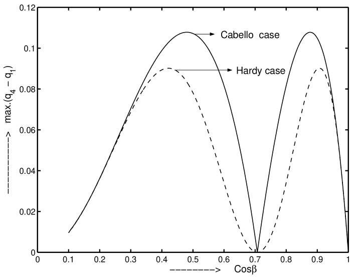
Figure 1: Comparison of the maximum probability of success between Hardy’s and Cabello’s case

Graph shows that for $\cos{\beta}\approx.7$ i.e for $\beta=\frac{\pi}{4}$ and for $\cos{\beta}=1$ i.e for $\beta=0$; maximum of $(q_{4}-q_{1})$ vanishes. This is as expected because these values of $\beta$ represent respectively the maximally entangled and product states for which Cabello’s argument does not run. For most of the other values of $\beta$ i.e for most of the other entangled states , maximum probability of success of Cabello’s argument in establishing their nonlocal feature is more than the maximum probability of success of hardy’s argument in doing the same.
As we have mentioned earlier (just before equation 28) that $\cos{(\phi_{D}+\phi_{E}-\gamma)}=1$ also optimizes $(q_{4}-q_{1})$. This also gives the same maximum value for $(q_{4}-q_{1})$as given by $\cos{(\phi_{D}+\phi_{E}-\gamma)}=-1$ but for $\theta_{D}=-\theta_{E}$.

Conclusion

In conclusion, here we have shown that maximally entangled states do not respond even to Cabello’s argument which is a relaxed one and is more general than Hardy’s argument. All other pure entangled states response to Cabello’s argument. These states also exhibit Hardy type nonlocality. But, interestingly for most of these nonmaximally entangled states, fraction of runs in which Cabello’s argument succeeds in demonstrating their nonlocal feature can be made more than the fraction of runs in which Hardy’s argument succeeds in doing the same. So it seems that in some sense, for demonstrating the nonlocal features of most of the entangled states, Cabello’s argument is a better candidate.
Appendix-
We want to optimize $(q_{4}-q_{1})$ given in equation $(28)$ with respect to $\theta_{D}$ and $\theta_{E}$ for a given $\beta$. Differentiating equation $(28)$ with respect to $\theta_{D}$ and equating it to zero, we have the following two equations

$$(\tan{\beta}\tan{\frac{\theta_{E}}{2}}+\tan{\frac{\theta_{D}}{2}})=0$$ (30)

and

$$(\tan{\beta}\tan{\frac{\theta_{E}}{2}}\tan{\frac{\theta_{D}}{2}}-1)(\tan^{2}{\beta}\tan^{2}{\frac{\theta_{E}}{2}}+1)(\tan^{2}{\beta}\tan^{2}{\frac{\theta_{D}}{2}}+1)^{2}=$$

$$(\tan^{2}{\beta}\sec^{2}{\frac{\theta_{D}}{2}})(\tan^{3}{\beta}\tan{\frac{\theta_{E}}{2}}\tan{\frac{\theta_{D}}{2}}-1)(\sec^{2}{\frac{\theta_{E}}{2}}\sec^{2}{\frac{\theta_{D}}{2}})$$ (31)

Similarly differentiating equation $(28)$ with respect to $\theta_{E}$ and equating it to zero, we have

$$(\tan{\beta}\tan{\frac{\theta_{D}}{2}}+\tan{\frac{\theta_{E}}{2}})=0$$ (32)

and

$$(\tan{\beta}\tan{\frac{\theta_{D}}{2}}\tan{\frac{\theta_{E}}{2}}-1)(\tan^{2}{\beta}\tan^{2}{\frac{\theta_{D}}{2}}+1)(\tan^{2}{\beta}\tan^{2}{\frac{\theta_{E}}{2}}+1)^{2}=$$

$$(\tan^{2}{\beta}\sec^{2}{\frac{\theta_{E}}{2}})(\tan^{3}{\beta}\tan{\frac{\theta_{D}}{2}}\tan{\frac{\theta_{E}}{2}}-1)(\sec^{2}{\frac{\theta_{D}}{2}}\sec^{2}{\frac{\theta_{E}}{2}})$$ (33)

Analyzing above four conditions we have

$$\theta_{D}=\theta_{E}$$

will give the optimal solution. Similarly for $cos{(\phi_{D}+\phi_{E}-\gamma)}=+1$, we will get same kind of results.

References

• [1] J.S. Bell, Physics 1, 195 (1964).
• [2] D.M. Greenberger, M.A. Horne and A. Zeilinger, in: Bell’s theorem, quantum theory and conceptions of the universe, edited by M. kafatos (Kluwer, Dordrecht, 1989) p. 69.
• [3] L. Hardy, Phys. Rev. Lett. 68, 2981 (1992).
• [4] L. Hardy, Phys. Rev. Lett. 71, 1665 (1993).
• [5] T. F. Jordan, Phys. Rev. A 50, 62 (1994).
• [6] A. Cabello, Phys. Rev. A 65, 032108 (2002).
• [7] Lin-mei Liang and Cheng-zu Li, Phys. Lett. A 335 , 371 (2005).
• [8] S. Kunkri and S.K. Choudhary Phys. Rev. A 72, 022348 (2005).
• [9] G. Kar, Phys. Rev. A 56, 1023 (1997).