A complete analysis of the Stern-Gerlach experiment using Pauli spinors

Abstract

The Stern-Gerlach experiment is the fundamental experiment in order to exhibit the quantization of spin and understand the measurement problem in quantum mechanics. However, although the Stern-Gerlach experiment plays an essential role in the teaching of quantum mechanics, no complete analysis of this experiment using Pauli spinors is presented in the pedagogical literature. This paper presents such an analysis and develops implications for the theory of quantum measurement.

We first propose an analytic expression of both the wave function and the probability density in the Stern-Gerlach experiment. Our explicit solution is obtained via a complete integration of the Pauli equation over time and space. The probability density evolution describes a slipping of the wave packet into two separate packets due to the measurement device, but it cannot account for impacts.

We therefore calculate the de Broglie-Bohm trajectories, which not only explain impacts naturally, but also accounts for the spin quantization following the magnetic field gradient. It is then possible to propose a clear explanation of measurement effects in the Stern-Gerlach experiment.

I Introduction

As they were studying the deviation of a silver atoms beam in a highly inhomogeneous magnetic field (cf. FIG. 1) Stern and Gerlach (1922)SternGerlach found empirical results which challenged common sense prediction. Instead of being scattered, the beam split into two symetric beams, which produced two spots of equal intensity on a screen, at equal distances from the axis of the original beam.

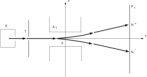
Figure 1: Schematic configuration of the Stern-Gerlach experiment.

This experiment motivated the introduction of spin quantization as an intrinsic magnetic moment. It also clearly exhibits the measurement problem in quantum mechanics, which remains an active field of study.Bohr ; Zurek ; Schlosshauer

This paper brings new elements, such as the analytic expression of the wave function and the probability density in the Stern-Gerlach experiment. The explicit solution is obtained via a complete integration of the Pauli equation over time and space. As far as we know, the analytic presentation of the Stern-Gerlach experiment in text-booksFeynmanCours is only given in time, not in space. The first explicit calculation in space and time of Stern-Gerlach experiment was given by Dewdney et alDewdney_1986 , but it remains incomplete, as is also incomplete their explicit solution in space and time of the Dirac equation.Challinor Recent presentations in space and time are only given with numerical simulations.Frana_1992

The analytic solution presented here gives an explicit expression of the probability density’s evolution in space, explaining the semi-classical presentation and showing the wave function separation. However, this continuous evolution in space of the wave packet into two wave packets does not account for the particle impacts. We therefore also calculate the de Broglie-Bohm trajectories deBroglie_1951 as we formerly did in the case of Young’s double slit experiment.Gondran_2005 These trajectories not only provide a natural explanation for the impact of particles, but also describe the spin quantization along the z-axis. It is then possible to propose a clear explanation of measurement in the Stern-Gerlach experiment.

The explicit solution in terms of Pauli spinors and the evolution of the probability density for the Stern-Gerlach experiment are presented in section 2. The de Broglie-Bohm trajectories, as defined by the interpretation of the Pauli equation by BohmBohm_1955 and Takabayasi,Takabayasi_1954 are simulated in section 3. Details of the calculations are provided in Appendix A.

II The probability density calculation in the Stern-Gerlach experiment

Silver atoms contained in the oven E (Fig. 1) are heated to a high temperature and escape through a narrow opening. A second aperture, T, selects those atoms whose velocity, $\textbf{v}_{0}$, is parallel to the y-axis. The atomic beam crosses the gap of the electromagnet $A_{1}$ before condensing on the screen, $P_{1}$ . The magnetic moments of the silver atoms before crossing the electromagnet are oriented randomly (isotropically). In the beam, we represent the atoms by their wave function ; one can suppose that at the entrance to the electromagnet, $A_{1}$, and at the initial time $t=0$, each atom prepared can be described by a Gaussian spinor in x and z:

$$\Psi^{0}(x,z)=(2\pi\sigma_{0}^{2})^{-\frac{1}{2}}e^{-\frac{(z^{2}+x^{2})}{4\sigma_{0}^{2}}}\binom{\cos\frac{\theta_{0}}{2}e^{i\frac{\varphi_{0}}{2}}}{i\sin\frac{\theta_{0}}{2}e^{-i\frac{\varphi_{0}}{2}}}.$$ (1)

The variable y will be treated in a classical way with $y=vt$. For a silver atom, one has $m=1.8\times 10^{-25}$ kg, $v_{0}=500$ m/s(with T=1000°K), $\sigma_{0}$=10^-4m.

In (1), $\theta_{0}$ and $\varphi_{0}$ are the polar angles characterizing the initial orientation of the magnetic moment, $\theta_{0}$ corresponds to the angle with the z-axis. This initial orientation being randomized, one can suppose that $\theta_{0}$ is drawn in a uniform way from $[0,\pi]$ and that $\varphi_{0}$ is drawn in a uniform way from $[0,2\pi]$. In this way, we give a model of a mixture of pure states.

The evolution of the spinor $\Psi=\binom{\psi_{+}}{\psi_{-}}$ in a magnetic field B is then given by the Pauli equation Platt :

$$i\hbar\left(\begin{array}[]{c}\frac{\partial\psi_{+}}{\partial t}\\ \frac{\partial\psi_{-}}{\partial t}\end{array}\right)=-\frac{\hbar^{2}}{2m}\nabla^{2}\left(\begin{array}[]{c}\psi_{+}\\ \psi_{-}\end{array}\right)+\mu_{B}\textbf{B}\boldsymbol{\sigma}\left(\begin{array}[]{c}\psi_{+}\\ \psi_{-}\end{array}\right)$$ (2)

where $\mu_{B}=\frac{e\hbar}{2m_{e}}$ is the Bohr magneton and where $\boldsymbol{\sigma}=(\sigma_{x},\sigma_{y},\sigma_{z})$ corresponds to the three Pauli matrices.

The particle first enters an electromagnetic field B directed along the z-axis, $B_{x}=B^{\prime}_{0}x$, $B_{y}=0$, $B_{z}=B_{0}-B^{\prime}_{0}z$, with $B_{0}=5$ Tesla and $B^{\prime}_{0}=\left|\frac{\partial B}{\partial z}\right|=10^{3}$ Tesla/m over a length $\Delta l=1~{}cm$. Such a vector B satisfies Maxwell’s equations, since $div(\textbf{B})=0$.

Once it leaves the magnetic field, the particle travels freely until it reaches the screen, $P_{1}$, placed a distance $D=20~{}cm$ beyond the magnet.

II.1 The Probability Density in the Magnetic Field

The particle stays within the magnetic field for a time $\Delta t=\frac{\Delta l}{v}=2\times 10^{-5}s$. During this time $[0,\Delta t]$, the spinor is (see Appendix A)

$$\Psi(x,z,t)=\left(\begin{array}[]{c}R_{+}e^{i\frac{S_{+}}{\hbar}}\\ R_{-}e^{i\frac{S_{-}}{\hbar}}\end{array}\right)\simeq\left(\begin{array}[]{c}\cos\frac{\theta_{0}}{2}(2\pi\sigma_{0}^{2})^{-\frac{1}{2}}e^{-\frac{(z-\frac{\mu_{B}B^{\prime}_{0}}{2m}t^{2})^{2}+x^{2}}{4\sigma_{0}^{2}}}e^{i\frac{\mu_{B}B^{\prime}_{0}tz-\frac{\mu^{2}_{0}B^{\prime 2}_{0}}{6m}t^{3}+\mu_{B}B_{0}t+\frac{\hbar\varphi_{0}}{2}}{\hbar}}\\ i\sin\frac{\theta_{0}}{2}(2\pi\sigma_{0}^{2})^{-\frac{1}{2}}e^{-\frac{(z+\frac{\mu_{B}B^{\prime}_{0}}{2m}t^{2})^{2}+x^{2}}{4\sigma_{0}^{2}}}e^{i\frac{-\mu_{B}B^{\prime}_{0}tz-\frac{\mu^{2}_{0}B^{\prime 2}_{0}}{6m}t^{3}-\mu_{B}B_{0}t-\frac{\hbar\varphi_{0}}{2}}{\hbar}}\end{array}\right)$$ (3)

Since the initial spinor direction is random, the atomic density, $\rho(z,t)$ is found by integrating $R_{+}^{2}+R_{-}^{2}$ on $(\theta_{0},\varphi_{0})$ and $x$ (notice that $R_{+}^{2}+R_{-}^{2}$ is independent of $\varphi_{0}$). So one gets:

$$\rho(z,t) =(2\pi\sigma_{0}^{2})^{-\frac{1}{2}}\frac{1}{2}\left(e^{-\frac{(z-\frac{\mu_{B}B^{\prime}_{0}}{2m}t^{2})^{2}}{2\sigma_{0}^{2}}}+e^{-\frac{(z+\frac{\mu_{B}B^{\prime}_{0}}{2m}t^{2})^{2}}{2\sigma_{0}^{2}}}\right).$$ (4)

II.2 The Probability Density after the Magnetic Field

After the magnetic field, at time $t+\Delta t$ $(t\geq 0)$, the spinor becomes (see Appendix A)

$$\Psi(x,z,t+\Delta t)=\left(\begin{array}[]{c}R_{+}e^{i\frac{S_{+}}{\hbar}}\\ R_{-}e^{i\frac{S_{-}}{\hbar}}\end{array}\right)\simeq\left(\begin{array}[]{c}\cos\frac{\theta_{0}}{2}(2\pi\sigma_{0}^{2})^{-\frac{1}{2}}e^{-\frac{(z-z_{\Delta}-ut)^{2}+x^{2}}{4\sigma_{0}^{2}}}e^{i\frac{muz+\hbar\varphi_{+}}{\hbar}}\\ i\sin\frac{\theta_{0}}{2}(2\pi\sigma_{0}^{2})^{-\frac{1}{2}}e^{-\frac{(z+z_{\Delta}+ut)^{2}+x^{2}}{4\sigma_{0}^{2}}}e^{i\frac{-muz+\hbar\varphi_{-}}{\hbar}}\end{array}\right)$$ (5)

where

$$z_{\Delta}=\frac{\mu_{B}B^{\prime}_{0}(\Delta t)^{2}}{2m}=10^{-5}m,~{}~{}~{}~{}~{}~{}u=\frac{\mu_{B}B^{\prime}_{0}(\Delta t)}{m}=1m/s.$$ (6)

One can deduce (as previously) the atom density $\rho$ at (z,$t+\Delta t$):

$$\rho(z,t+\Delta t) =(2\pi\sigma_{0}^{2})^{-\frac{1}{2}}\frac{1}{2}\left(e^{-\frac{(z-z_{\Delta}-ut)^{2}}{2\sigma_{0}^{2}}}+e^{-\frac{(z+z_{\Delta}+ut)^{2}}{2\sigma_{0}^{2}}}\right).$$ (7)

Figure  2 shows the probability density of the silver atoms as a function of z at several values of t ( the plots are labelled with $y=vt$). The beam separation does not appear at the end of the magnetic field (1 cm), but 10 cm further along.

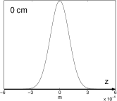
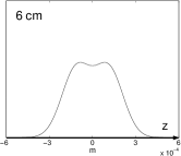
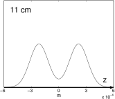
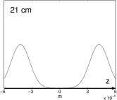
Figure 2: Evolution of the probability density of silver atoms.

In equations (4) and (7) one recognizes classical trajectories:

$$z_{\pm}=\{\pm\frac{\mu_{B}B^{\prime}_{0}t^{2}}{m}~{}~{}for~{}~{}t\in[0,\Delta t];\pm z_{\Delta}\pm ut~{}~{}for~{}~{}\Delta t+t(t\geq 0)\}$$ (8)

corresponding to particles with magnetic moments of $\mu_{z}=\mu_{B}$ and $\mu_{z}=-\mu_{B}$ respectively. The trajectories are parabolic inside the magnetic field and linear after. The two spots $N^{+}$ and $N^{-}$ become separated when $z_{+}-z_{-}\gtrapprox 4\sigma_{0}$, which occurs at the separation time

$$t_{s}\simeq\frac{3\sigma_{0}}{u}=\frac{3\sigma_{0}mv}{\mu_{B}B^{\prime}_{0}\Delta l}=\frac{6\sigma_{0}mm_{e}v}{e\hbar B^{\prime}_{0}\Delta l}=3\times 10^{-4}s.$$ (9)

Statistically, everything happens as if the atom’s moment were quantified in two parts: one half of the particles having $\mu_{z}=\mu_{B}$ and the other half having $\mu_{z}=-\mu_{B}$. This result explains why the semi-classical description of this Stern-Gerlach experiment is usually used. This semi-classical description starts from the quantization of spin and deduces from Ehrenfest’s Theorem the average trajectories of the spinors with initial spinors $\Psi_{+}^{0}=(2\pi\sigma_{0}^{2})^{-\frac{1}{2}}e^{-\frac{(z^{2}+x^{2})}{4\sigma_{0}^{2}}}\binom{1}{0}$ and $\Psi_{-}^{0}=(2\pi\sigma_{0}^{2})^{-\frac{1}{2}}e^{-\frac{(z^{2}+x^{2})}{4\sigma_{0}^{2}}}\binom{0}{1}$ respectively. Note that this is a statistical interpretation, and the individuality of the atoms represented by the angles $\theta_{0}$ and $\varphi_{0}$ is lost. However experimentally, one does not observe directly the wave function, but individual impacts of the silver atoms on the $P_{1}$ screen. The usual explanation of these individual impacts on the screen is decoherence, Zurek ; Schlosshauer caused by the interaction with the measurement device. Here, the evolution of the probability density given by equations (4) and (7) correctly describes a separation of the wave packet into two packets thanks to the measurement device, but cannot describe the individual positions of these impacts.

III Impacts and Quantization explained by trajectories

To explain individual impacts, we simulate the silver atom trajectories in the de Broglie-Bohm interpretation just as we did Gondran_2005 for the neon atoms in the Young’s double slit experiment. In this unusual presentation of the Quantum Mechanics results, the particle is represented not only by its wave function, but also by the position of its center-of-mass.

Indeed at the first instant, the wave function $\Psi^{0}(x,z)$ gives the initial probability density $\Psi^{0}(x,z)$. This density, which doesn’t depend on $\hbar$, is the classic presence density of a silver atom. So in classic mechanics, one does have an undetermination on the atom position, and in order to describe its evolution, it is necessary to precise its initial position. The principle of the De Broglie-Bohm interpretation is to do the same in quantum mechanics.

So, in the Pauli equation case (2), atoms have trajectories that are defined by using the center-of-mass velocity $\textbf{v}(x,y,z,t)$ givenBohm_1955 ; Takabayasi_1954 by :

$$\textbf{v}=\frac{\hbar}{2m\rho}Im{(\Psi^{\dagger}\boldsymbol{\nabla}\Psi)}+\frac{\hbar}{2m\rho}rot(\Psi^{\dagger}\boldsymbol{\sigma}\Psi)$$ (10)

where $\Psi^{\dagger}=[\psi_{+}^{*},\psi_{-}^{*}]$.

Let us show how this interpretation gives the same results as the Copenhagen school. One verifiesBohm_1955 ; Takabayasi_1954 that with v given by (10), the probability density $\rho(x,y,z,t)=\Psi^{\dagger}\Psi=|\Psi(x,y,z,t)|^{2}$ of the $\Psi$ spinor solution of the Pauli equation (2) satisfies the Madelung continuity equation:

$$\frac{\partial\rho}{\partial t}+div(\rho\textbf{v})=0.$$

One can deduce from it, that if a particle family with the initial probability density $\rho_{0}(x,y,z)$ follows the de Broglie-Bohm trajectories, its probability density at the t time, will be $\rho(x,y,z,t)$.

Thus, these two interpretations give statistically identical results, but the de Broglie-Bohm interpretation predicts the position of individual impacts as well. We shall see that these trajectories also explain the spin quantization following the magnetic field gradient.

In equation (10), the last term $\frac{\hbar}{2m\rho}rot(\Psi^{\dagger}\boldsymbol{\sigma}\Psi)$ corresponds to the Gordon current. Its contribution to velocity is here negligible. We will therefore not take it into account from now.

In the de Broglie-Bohm interpretation, the individual particle is not only described by its wave function, but by its initial position $(x_{0},z_{0},y_{0}=0)$ as well. So, trajectories in x and z are given by the differential equations:

$$\frac{dx}{dt}=\frac{1}{2m}\frac{\partial(S_{+}+S_{-})}{\partial x}+\frac{1}{2m}\frac{\partial(S_{+}-S_{-})}{\partial x}\cos\theta$$ (11)

$$\frac{dz}{dt}=\frac{1}{2m}\frac{\partial(S_{+}+S_{-})}{\partial z}+\frac{1}{2m}\frac{\partial(S_{+}-S_{-})}{\partial z}\cos\theta$$ (12)

with $\tan\frac{\theta}{2}=\frac{R_{-}}{R_{+}}$.

A silver atom with a polarization ($\theta_{0}$,$\varphi_{0}$) and a position $z_{0}$ at the entrance of the electro-magnet $A_{1}$ will satisfy the differential equation in the $[0,\Delta t]$ period:

$$\frac{dz}{dt}=\frac{\mu_{B}B^{\prime}_{0}t}{m}cos\theta(z,t)~{}~{}~{}~{}with~{}~{}~{}~{}~{}~{}\tan\frac{\theta(z,t)}{2}=\tan\frac{\theta_{0}}{2}e^{-\frac{\mu_{B}B^{\prime}_{0}t^{2}z}{2m\sigma_{0}^{2}}}$$ (13)

and for the $\Delta t+t$ ($t\geq 0$) period:

$$\frac{dz}{dt}=u\frac{\tanh(\frac{(z_{\Delta}+ut)z}{\sigma_{0}^{2}})+\cos\theta_{0}}{1+\tanh(\frac{(z_{\Delta}+ut)z}{\sigma_{0}^{2}})\cos\theta_{0}}~{}~{}~{}~{}and~{}~{}~{}~{}~{}~{}\tan\frac{\theta(z,t)}{2}=\tan\frac{\theta_{0}}{2}e^{-\frac{(z_{\Delta}+ut)z}{\sigma_{0}^{2}}}.$$ (14)

Figure 3 presents a plot in the x,y plane of a set of 10 silver atom trajectories with the initial polarization $(\theta_{0}=\frac{\pi}{3},\varphi_{0}=0)$ and whose initial position $z_{0}$ has been randomly chosen from a Gaussian distribution with standard deviation $\sigma_{0}$. The spin orientations $\theta(z,t)$ are represented by arrows.

Figure 3 presents, for a silver atom with the initial polarization $(\theta_{0}=\frac{\pi}{3},\varphi_{0}=0)$, a plot in the x,y plane of a set of 10 trajectories whose initial position $z_{0}$ has been randomly chosen from a Gaussian distribution with standard deviation $\sigma_{0}$. The spin orientations $\theta(z,t)$ are represented by arrows.

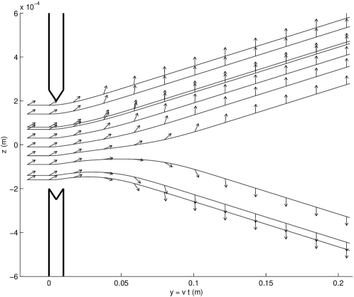
Figure 3: Ten silver atom trajectories with initial polarization $(\theta_{0}=\frac{\pi}{3})$ and initial position $z_{0}$; Arrows represent the spin orientation $\theta(z,t)$ along the trajectories.

One can notice that the final orientation, obtained after the separation time $t_{s}$, will depend on the initial particle position $z_{0}$ in the wave packet and on the initial angle $\theta_{0}$ of the atom magnetic moment with the axis z.

We obtain $+\frac{\pi}{2}$ if $z_{0}>z^{\theta_{0}}$ and $-\frac{\pi}{2}$ if $z_{0}<z^{\theta_{0}}$ with

$$z^{\theta_{0}}=\sigma_{0}F^{-1}(\sin^{2}\frac{\theta_{0}}{2})$$ (15)

where F is the cumulative distribution function of the standard normal distribution.

So besides explaining the position of impacts, this simulation shows that it is possible to give a simple interpretation of quantization on z-axis.

Figure 4 presents a plot in the x,y plane of a set of 10 silver atom trajectories whose initial characteristics $(\theta_{0},\varphi_{0},z_{0})$ have been randomly chosen: $\theta_{0}$ and $\varphi_{0}$ from an uniform distribution and $z_{0}$ from a Gaussian distribution with standard deviation $\sigma_{0}$. The spin orientations $\theta(z,t)$ are represented by arrows.

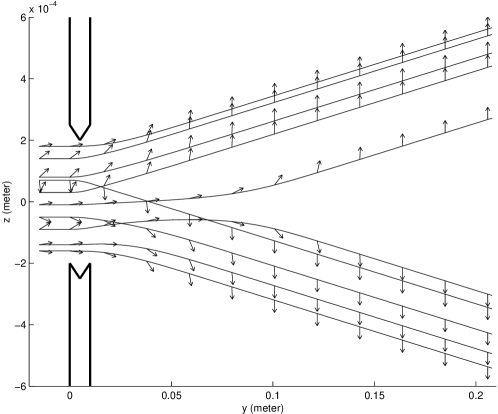
Figure 4: 10 silver atom trajectories after the electro-magnet; Arrows represent the spin orientation $\theta(z,t)$ along the trajectories.

IV Conclusion

It is now possible to propose the following interpretation of measurement in quantum mechanics. There certainly exists an interaction with the measuring apparatus as it is classically explained, and there exists a minimum delay necessary for the measurement $t_{s}=\frac{3\sigma_{0}}{u}$. Yet we believe that this measurement and this delay do not have the meanings that are classically attributed to them. In the present case, the measuring apparatus itself gives the orientation of the spin either in the direction of field, or in the direction opposite to the field, depending on the position of the particle in the wave packet. The measuring delay is then the time which is necessary for the particle to point its spin to the final direction.

Let us notice that in this numerical study of the Stern-Gerlach experiment we didn’t need any of the classical postulates of measurement in quantum mechanics, such as eigenvalues of the Hamiltonian or wave packet reduction. These two postulates may account for experimental results, but they do not give any idea of the transitions that lead to these results. Instead we only used the quantum mechanics equations (Pauli equation) and made only one hypothesis : the centers of mass of the atoms in the atomic beam are spacially distributed according to the density given by the wave function, and follow paths that are compatible with the continuity equation (De Broglie-Bohm hypothesis). From this one and only hypothesis, we provided altogether:

- a simple explanation of the position of the particle impacts;

- a simple explanation of the spin quantization along the measurement axis ;

- an simple explanation of the transition towards the Hamiltonian eigenvalues.

Appendix A Calculating the spinor of the Stern-Gerlach experiment

In the magnetic field $B=(B_{x},0,B_{z})$, the Pauli equation (2) gives coupled Schrödinger equations for each spinor component

$$i\hbar\frac{\partial\psi_{\pm}}{\partial t}(x,z,t)=-\frac{\hbar^{2}}{2m}\nabla^{2}\psi_{\pm}(x,z,t)\pm\mu_{B}(B_{0}-B_{0}^{\prime}z)\psi_{\pm}(x,z,t)\mp i\mu_{B}B_{0}^{\prime}x\psi_{\mp}(x,z,t).$$ (16)

If one effects the transformation Platt

$$\psi_{\pm}(x,z,t)=\exp(\pm\frac{i\mu_{B}B_{0}t}{\hbar})\overline{\psi}_{\pm}(x,z,t)$$

equation (16) becomes

$$i\hbar\frac{\partial\overline{\psi}_{\pm}}{\partial t}(x,z,t)=-\frac{\hbar^{2}}{2m}\nabla^{2}\overline{\psi}_{\pm}(x,z,t)\mp\mu_{B}B^{\prime}_{0}z\overline{\psi}_{\pm}(x,z,t)\mp i\mu_{B}B^{\prime}_{0}x\overline{\psi}_{\mp}(x,z,t)\exp(\pm i\frac{2\mu_{B}B_{0}t}{\hbar})$$

The coupling term oscillates rapidly with frequency $\omega=\frac{2\mu_{B}B_{0}}{\hbar}=1,4\times 10^{11}s^{-1}$. Since $|B_{0}|\gg|B^{\prime}_{0}z|$ and $|B_{0}|\gg|B^{\prime}_{0}x|$, the period of oscillation is short compared to the motion of the packet along its trajectory. Avering over a period that is long compared to the period of oscillation, causes the coupling term to vanish, yielding Platt

$$i\hbar\frac{\partial\overline{\psi}_{\pm}}{\partial t}(x,z,t)=-\frac{\hbar^{2}}{2m}\nabla^{2}\overline{\psi}_{\pm}(x,z,t)\mp\mu_{B}B^{\prime}_{0}z\overline{\psi}_{\pm}(x,z,t).$$

The initial wave function $\overline{\psi}_{\pm}^{0}(x,z)=\psi_{\pm}^{0}(x,z)=\psi_{x}^{0}(x)\psi_{\pm}^{0}(z)$ with $\psi_{x}^{0}(x)=(2\pi\sigma_{0}^{2})^{-\frac{1}{4}}e^{-\frac{x^{2}}{4\sigma_{0}^{2}}}$, $\psi_{+}^{0}(z)=(2\pi\sigma_{0}^{2})^{-\frac{1}{4}}e^{-\frac{z^{2}}{4\sigma_{0}^{2}}}\cos\frac{\theta_{0}}{2}e^{i\frac{\varphi_{0}}{2}}$ and $\psi_{-}^{0}(z)=(2\pi\sigma_{0}^{2})^{-\frac{1}{2}}e^{-\frac{z^{2}}{4\sigma_{0}^{2}}}i\sin\frac{\theta_{0}}{2}e^{-i\frac{\varphi_{0}}{2}}$ allows a separation of variables x and z. Then we can compute explicitly the preceding equations for all t in $[0,\Delta t]$ with $\Delta t=\frac{\Delta l}{v}=2\times 10^{5}s$.

We obtain: $\overline{\psi}_{\pm}(x,z,t)=\overline{\psi}_{x}(x,t)\overline{\psi}_{\pm}(z,t)$ with

$$\overline{\psi}_{x}(x,t)=(2\pi\sigma_{t}^{2})^{-\frac{1}{4}}e^{-\frac{x^{2}}{4\sigma_{t}^{2}}}\exp\frac{i}{\hbar}[-\frac{\hbar}{2}\tan^{-1}(\frac{\hbar t}{2m\sigma_{0}^{2}})+\frac{x^{2}\hbar^{2}t^{2}}{8m\sigma_{0}^{2}\sigma_{t}^{2}}]$$ (17)

$$\overline{\psi}_{+}(z,t)=\psi_{K}(z,t)\cos\frac{\theta_{0}}{2}e^{i\frac{\varphi_{0}}{2}}~{}~{}~{}~{}~{}and~{}~{}K=-\mu_{B}B^{\prime}_{0}$$

$$\overline{\psi}_{-}(z,t)=\psi_{K}(z,t)i\sin\frac{\theta_{0}}{2}e^{-i\frac{\varphi_{0}}{2}}~{}~{}~{}~{}~{}and~{}~{}K=+\mu_{B}B^{\prime}_{0}$$

$\sigma_{t}^{2}=\sigma_{0}^{2}+\left(\frac{\hbar t}{2m\sigma_{0}}\right)^{2}$ and

$$\psi_{K}(z,t)=(2\pi\sigma_{t}^{2})^{-\frac{1}{4}}e^{-\frac{(z+\frac{Kt^{2}}{2m})^{2}}{4\sigma_{t}^{2}}}\exp\frac{i}{\hbar}[-\frac{\hbar}{2}\tan^{-1}(\frac{\hbar t}{2m\sigma_{0}^{2}})-Ktz-\frac{K^{2}t^{3}}{6m}+\frac{(z+\frac{Kt^{2}}{2m})^{2}\hbar^{2}t^{2}}{8m\sigma_{0}^{2}\sigma_{t}^{2}}].$$ (18)

Equations (17) and (18) are classical results.Feynman

The experimental conditions give $\frac{\hbar\Delta t}{2m\sigma_{0}}=4\times 10^{-11}~{}m\ll\sigma_{0}=10^{-4}~{}m$. We deduce the approximations $\sigma_{t}\simeq\sigma_{0}$, $\overline{\psi}_{x}(x,t)\simeq\psi_{x}^{0}(x)=(2\pi\sigma_{0}^{2})^{-\frac{1}{4}}e^{-\frac{x^{2}}{4\sigma_{0}^{2}}}$ and

$$\overline{\psi}_{K}(z,t)\simeq(2\pi\sigma_{0}^{2})^{-\frac{1}{4}}e^{-\frac{(z+\frac{Kt^{2}}{2m})^{2}}{4\sigma_{0}^{2}}}\exp\frac{i}{\hbar}[-Ktz-\frac{K^{2}t^{3}}{6m}].$$ (19)

At the end of the magnetic field, at time $\Delta t$, the spinor equals to

$$\Psi(x,z,\Delta t)=\psi_{x}(x,\Delta t)\left(\begin{array}[]{c}\psi_{+}(z,\Delta t)\\ \psi_{-}(z,\Delta t)\end{array}\right)$$ (20)

with

$$\psi_{+}(z,\Delta t)=(2\pi\sigma_{0}^{2})^{-\frac{1}{4}}e^{-\frac{(z-z_{\Delta})^{2}}{4\sigma_{0}^{2}}+\frac{i}{\hbar}muz}\cos\frac{\theta_{0}}{2}e^{i\varphi_{+}}$$

$$\psi_{-}(z,\Delta t)=(2\pi\sigma_{0}^{2})^{-\frac{1}{4}}e^{-\frac{(z+z_{\Delta})^{2}}{4\sigma_{0}^{2}}-\frac{i}{\hbar}muz}i\sin\frac{\theta_{0}}{2}e^{i\varphi_{-}}$$

$$z_{\Delta}=\frac{\mu_{B}B^{\prime}_{0}(\Delta t)^{2}}{2m},~{}~{}~{}~{}~{}~{}u=\frac{\mu_{0}B^{\prime}_{0}(\Delta t)}{m}~{}~{}~{}~{}and$$

$$\varphi_{+}=\frac{\varphi_{0}}{2}-\frac{\mu_{B}B_{0}\Delta t}{\hbar}-\frac{K^{2}(\Delta t)^{3}}{6m\hbar};~{}~{}~{}~{}\varphi_{-}=-\frac{\varphi_{0}}{2}+\frac{\mu_{0}B_{0}\Delta t}{\hbar}-\frac{K^{2}(\Delta t)^{3}}{6m\hbar}.$$

We remark that the crossing through the magnetic field gives the equivalent of a velocity $+u$ in the direction $0z$ to the function $\psi_{+}$ and a velocity $-u$ to the function $\psi_{-}$. Then we have a free particle with the initial wave function (20). The Pauli equation resolution gives again $\psi_{\pm}(x,z,t)=\psi_{x}(x,t)\psi_{\pm}(z,t)$ and with the experimental conditions we have $\psi_{x}(x,t)\simeq(2\pi\sigma_{0}^{2})^{-\frac{1}{4}}e^{-\frac{x^{2}}{4\sigma_{0}^{2}}}$ and

$$\psi_{+}(z,t+\Delta t)\simeq(2\pi\sigma_{0}^{2})^{-\frac{1}{4}}e^{-\frac{(z-z_{\Delta}-ut)^{2}}{4\sigma_{0}^{2}}+\frac{i}{\hbar}(muz-\frac{1}{2}mu^{2}t+\hbar\varphi_{+})}\cos\frac{\theta_{0}}{2}$$

$$\psi_{-}(z,t+\Delta t)\simeq(2\pi\sigma_{0}^{2})^{-\frac{1}{4}}e^{-\frac{(z+z_{\Delta}+ut)^{2}}{4\sigma_{0}^{2}}+\frac{i}{\hbar}(-muz-\frac{1}{2}mu^{2}t+\hbar\varphi_{-})}i\sin\frac{\theta_{0}}{2}$$

References

(1)
Von W. Gerlach and O. Stern, "Der Experimentelle Nachweis des
Magnetischen Moments des Silberatoms", (Zeit. Phys.8, 110, 1921);
(Zeit. Phys.9, 349, 1922)
(2)
N. Bohr, Discussion with Einstein and Epistemological
Problems in Atomic Physics, in Albert Einstein:
Philosopher-Scientist, edited by P.A. Schlipp (The Library of
Living Philosophers, Evanston, 1949), pp.200-241.
(4)
M. Schlosshauer, "Decoherence, the Measurement Problem, and
Interpretations of Quantum Mechanics", Rev. Mod. Phys.
76, n°4 (2003) 1267-1305 ; quant-ph/0312059.
(5)
R. P. Feynman, R. B. Leighton, and M. Sands, The Feynman
Lectures on Physics (Addison-Wesley, New York, 1965); C.
Cohen-Tannoudji, B. Diu, and F. Laloë, Quantum Mechanics
(Wiley, New York, 1977); J. J. Sakurai, Modern quantum
Mechanics (New-York: Addison-Weslay, 1985).
(6)
C. Dewdney, P.R. Holland, and A. Kypianidis, "What happens in a
spin measurement ?", Phys. Lett. A, 119(6), 259-267
(1986).
(7)
A. Challinor, A. Lasenby, S. Gull, and Chris Doran, "A
relativistic causal account of a spin measurement", Phys. Lett. A
218, 128-138 (1996).
(8)
H. N. Frana, T. W. Marshall, E. Santos and E. J. Watson, Phys.
Rev. A46 (1992) 2265-70; B.M.Garraway and S.Stenholm,
Phys. Rev. A60 (1999) 63-79.
(9)
L. de Broglie, J. de Phys. 8, 225-241 (1927); Une
tentative d’interprétation causale et non linéaire de la mécanique
ondulatoire, Gauthier-Villars, Paris, 1951; D. Bohm, "A suggested
interpretation of the quantum theory in terms of "hidden"
variables", Physical Review, 85, 166-193(1952). See also:
D. Bohm,and B.J. Hiley, The Undivided Universe,
(Routledge, London and New York, 1993); P.R. Holland , The
quantum Theory of Motion, (Cambridge University Press, 1993).
(10)
M. Gondran, and A. Gondran , "Numerical simulation of the
double-slit interference with ultracold atoms", Am. J. Phys.
73, 6, 2005.
(11)
D. Bohm, R. Schiller, and J. Tiomno, "A causal interpretation of
the Pauli equation" - Nuovo Cim. supp. 1, 48-66 (1955);
Nuovo Cim. supp. 1, 67-91 (1955).
(12)
T. Takabayasi, "On the Formulation of Quantum Mechanics associated
with Classical Pictures", Prog. Theor. Phys. 8, n°2, 143
(1952); " The Formulation of Quantum Mechanics in terms of
Ensemble in Phase Space", Prog. Theor. Phys. 11, n°4-5,
341 (1954); "The vector Representation of Spinning particle in the
Quantum Theory,1", Prog. Theor. Phys. 14, n°4, 283
(1955).
(13)
D.E. Platt, "A modern analysis of the Stern-Gerlach experiment",
Am. J. Phys. 60 (4), April 1992.
(14)
R. Feynman and A. Hibbs, Quantum Mechanics and Paths
Integrals, McGraw-Hill, Inc.,p. 63, problem 3-9 ( 1965); G.
Vandegrift, "Accelerating wave packet solution to Schrödinger’s
equation", Am. J. Phys. 68, 576-7, 2000.