Quantum computation with abelian anyons on the honeycomb lattice

Abstract

We consider a two-dimensional spin system that exhibits abelian anyonic excitations. Manipulations of these excitations enable the construction of a quantum computational model. While the one-qubit gates are performed dynamically the model offers the advantage of having a two-qubit gate that is of topological nature. The transport and braiding of anyons on the lattice can be performed adiabatically enjoying the robust characteristics of geometrical evolutions. The same control procedures can be used when dealing with non-abelian anyons. A possible implementation of the manipulations with optical lattices is developed.

Topological models address in the most sufficient way the problem of decoherence, which is the main obstacle in the realization of quantum computation Kitaev_97 ; Freedman ; Mochon ; Bonesteel . This is achieved by encoding information in the statistical properties of non-abelian anyons. Hence, information remains unaffected by temperature or local perturbation as long as the nature of the anyons does not change. Subsequently, information can be processed by braiding anyons, an evolution which is topologically protected from control errors. Nevertheless, due to their exotic nature these models are hard to realize physically. To approach this problem we construct a simple model for quantum computation with topological characteristics that can be implemented easier than the fully topological quantum computer. The simplest case is to identify the topological phase arising from the statistics of abelian anyons with a two-qubit gate Lloyd . In this scenario qubit encoding and one-qubit gates can be performed in the usual dynamical way.

The purpose of this letter is twofold. First, we propose a physically realizable model for the generation and detection of abelian anyons. The latter can be subsequently used to perform quantum computation that has a topologically protected two-quit gate. Second, we develop the test ground for the generalization to the more demanding non-abelian case where topological quantum memory or computation can be performed. Indeed, the main ingredients of the abelian case, such as the creation of anyons, their braiding and their subsequent measurement can be carried through to the case of non-abelian anyons.

While the ideas here can be applied to a variety of different setups Paredes ; Bombin we shall employ a particular physical model, namely a two dimensional spin-1/2 system where the spins are located at the vertices of a honeycomb lattice Kitaev . The spins are set to interact with each other via the following Hamiltonian

$$H=-J_{x}\sum_{\text{x-links}}\sigma_{j}^{x}\sigma_{k}^{x}-J_{y}\sum_{\text{y-links}}\sigma_{j}^{y}\sigma_{k}^{y}-J_{z}\sum_{\text{z-links}}\sigma_{j}^{z}\sigma_{k}^{z}$$ (1)

where “x-links”, “y-links” and “z-links” label the three different link directions of the honeycomb lattice as depicted in Figure 1. It has been shown Kitaev that this model exhibits two main distinctive phases. For $|J_{x}|+|J_{y}|\geq|J_{z}|$, $|J_{y}|+|J_{z}|\geq|J_{x}|$ and $|J_{z}|+|J_{x}|\geq|J_{y}|$ a gapless sector appears that supports non-abelian excitations, while the violation of any of the three inequalities leads to a gap. Here we shall focus on the latter phase for a concrete choice of couplings, namely $|J_{z}|>|J_{x}|+|J_{y}|$. As we shall explicitely see here this phase is equivalent to Kitaev’s toric code which exhibits three distinguished species of particle excitations above the ground state $0$, namely a fermion, $\epsilon$, and two bosons, the chargeon, $e$, and the magnon, $m$ Kitaev_97 . Interestingly, exchanges between different particles reveals their anyonic character.

To identify the properties of the abelian phase in the honeycomb lattice it is instructive to employ perturbation theory Kitaev . Nevertheless, the discrete qualitative properties of the model will stay the same even beyond the perturbative approximation Jiannis . Consider the coupling regime where $J_{x},J_{y},J_{z}\geq 0$ and $J_{z}\gg J_{x},J_{y}$. The dominant $z$-interaction has as lower eigenstates $\left|\,\tilde{\uparrow}\right\rangle\equiv\left|\,\uparrow\uparrow\right\rangle$ and $\left|\,\tilde{\downarrow}\right\rangle\equiv\left|\,\downarrow\downarrow\right\rangle$ for each $z$-link. The Pauli operators that act on these states are given by $\tilde{\sigma}^{x}\equiv\sigma^{x}\sigma^{x}$, $\tilde{\sigma}^{y}\equiv\sigma^{y}\sigma^{x}\approx\sigma^{x}\sigma^{y}$ and $\tilde{\sigma}^{z}\equiv\sigma^{z}1\approx 1\sigma^{z}$, where ‘$\approx$’ stands for equality in the space spanned by the $\left|\,\tilde{\uparrow}\right\rangle$ and $\left|\,\tilde{\downarrow}\right\rangle$ vectors. Considering up to fourth order in perturbation theory, the Hamiltonian (1) becomes

$$H\simeq-{J_{x}^{2}J_{y}^{2}\over 16J_{z}^{3}}\sum_{p}\tilde{\sigma}^{y}_{1}\tilde{\sigma}^{z}_{2}\tilde{\sigma}^{y}_{3}\tilde{\sigma}^{z}_{4}\equiv-J_{\text{eff}}\sum_{p}Q_{p},$$ (2)

where an irrelevant constant term has been omitted. The summation in (2) is over all plaquettes of the lattice, while the lower indices of the Pauli operators denote the position of the effective spins around the plaquette, $p$, starting from the left and moving clockwise (see Figure 1).

This Hamiltonian is unitarily equivalent to the more familiar Kitaev’s toric code Kitaev_97 , but here we shall work with Hamiltonian (2). Before studying the particle excitations we first determine the ground state, $\left|\,0\right\rangle$. Since $Q_{p}^{\dagger}=Q_{p}$ and $Q_{p}^{2}=1$, the eigenvalues of $Q_{p}$ are $\pm 1$ and since $[Q_{p},Q_{p^{\prime}}]=0$ for all $p$, $p^{\prime}$, the lowest energy state has to satisfy $Q_{p}\left|\,0\right\rangle=\left|\,0\right\rangle$ for all $p$. Excitations of Hamiltonian (2) are given by relaxing this requirement at some plaquettes. For periodic boundary conditions we have $\prod_{p}Q_{p}=1$ at all times, hence, excitations should appear in pairs. For open boundary conditions single excitations are possible, where the other part of the pair can be considered to be outside the system. Nevertheless, for manipulations away from the boundary we may assume that the generated particles come in pairs.

Figure 1: The honeycomb lattice with the three different types of links $x$, $y$ and $z$. The distribution of the four spin interaction, $Q_{p}$, is indicated. Possible positions of the excitation pairs produced by rotations of effective spins.

Consider a rotation $\tilde{\sigma}^{z}$ applied on a certain $z$-link. As $\tilde{\sigma}^{z}$ anticommutes with the $Q_{p}$ interactions of the plaquettes on its left and on its right it will increase the energy of these plaquettes by $\Delta E=2J_{\text{eff}}$. Similarly, if we perform a rotation $\tilde{\sigma}^{y}$, then the energy of the plaquettes above and below increases by $\Delta E$. If a rotation $i\tilde{\sigma}^{x}$ is performed, then all four neighboring plaquettes obtain an energy increase of $\Delta E$ each. Hence, the low lying energy eigenstates are elementary pairs of excitations given by

$$\left|\,Z\right\rangle=\tilde{\sigma}_{j}^{z}\left|\,0\right\rangle\,\,\,\,\,\,\text{and}\,\,\,\,\,\,\left|\,Y\right\rangle=\tilde{\sigma}_{j}^{y}\left|\,0\right\rangle.$$ (3)

These excitations live in appropriate neighboring plaquettes as indicated in Figure 1. Moreover, one can combine such pairs of excitations in a chain of $\tilde{\sigma}^{z}$ and $\tilde{\sigma}^{y}$ rotations to create two excitations at the end points of an arbitrary string $s$. Similarly, one can define a pair of fermionic excitations, $\left|\,X\right\rangle$, as

$$\left|\,X[s]\right\rangle=\prod_{j\in s}i\tilde{\sigma}_{j}^{x}\left|\,0\right\rangle,$$ (4)

where $s$ is the path along which $\tilde{\sigma}^{x}$ rotations are performed in such a way as interweaving of the constituent $\tilde{\sigma}^{y}$ and $\tilde{\sigma}^{z}$ paths is achieved. The eigenvalues of the energy of the $Y$ and $Z$ excitations have an energy gap above the ground state given by $\Delta E=4J_{\text{eff}}$, while for the $X$ excitation the energy gap is double. Note that, the eigenvalue of the energy of each excitation is independent of the length of the string, $s$, as the contributions to the energy come only from its two end-points.

From these definitions one can easily deduce the fusion rules $X\times X=Y\times Y=Z\times Z=1$, $X\times Y=Z$, $Y\times Z=X$ and $Z\times X=Y$, where $1$ denotes the vacuum. Indeed, two successive identical Pauli rotations ($X$, $Y$ or $Z$), that correspond to superposing two pairs of the same excitations, will give the identity operation. The generation of an $X$-particle out of the fusion of $Y$- and $Z$-particles follows straightforwardly from the property $\tilde{\sigma}^{y}\tilde{\sigma}^{z}=i\tilde{\sigma}^{x}$. Furthermore, from definitions (3) and (4) one can deduce the statistics of these particles. Exchanging two $X$-particles results in a complete overlap of their strings at $2(2k+1)$ sites, where $k$ is an inteeger, giving eventually $(i\tilde{\sigma}^{x})^{2}=-1$ as an overall factor that reveals their fermionic character. To probe the anyonic character we circulate an $X$-particle around a single $Y$- or $Z$-particle. This loop that corresponds to two consecutive exchanges gives a string operator that anticommutes with the string of the $Y$- or $Z$-particles, due to the anticommuting properties of the Pauli operators at the site of their intersection. Hence, a minus sign will be produced revealing that the $X$ and $Y$ or $Z$ particles behave as anyons with respect to each other with statistical angle $\theta=\pi/2$. Note, that due to the undetermined structure of the strings for the $Y$ and $Z$ particles it is not straightforward to deduce their statistical properties.

In order to use this setup to perform quantum computation we encode the states of a qubit in the space of excitations of the system, namely $\left|\,0_{L}\right\rangle=\left|\,X\right\rangle$ and $\left|\,1_{L}\right\rangle=\left|\,Y\right\rangle$ (or $\left|\,1_{L}\right\rangle=\left|\,Z\right\rangle$ depending on the position of the excitation). To manipulate these states we place them in neighboring plaquettes. A one-qubit rotation, e.g. of the $\left|\,0_{L}\right\rangle$ state, can then be performed by an appropriate $z$-rotation, $e^{-i\tilde{\sigma}^{z}\theta}\left|\,X\right\rangle=\cos\theta\left|\,X\right\rangle-i\sin\theta\left|\,Y\right\rangle$. The $\tilde{\sigma}^{z}=\sigma^{z}1$ rotation is performed at the effective spin that connects the pair of $X$ particles. A relative phase between the two states $\left|\,0_{L}\right\rangle$ and $\left|\,1_{L}\right\rangle$ can be generated by changing the relative self-energy of the corresponding excitations. Hence, a general one-qubit gate can be obtained in the usual dynamical way.

The realisation of a two qubit gate requires braiding of the anyonic particles. To transport the anyons around the two dimensional lattice one can create a trapping potential well with depth $V$ for each anyon. This can be achieved by reducing the coupling $J_{\text{eff}}$ by $V$ at the corresponding hexagon. A simple implementation is by increasing the couplings of the two $z$-links that surround a particular hexagon occupied by the anyon to the value $J_{z}^{\prime}$. Thus, the effective coupling becomes $J_{\text{eff}}^{\prime}=J_{x}^{2}J_{y}^{2}/(4(J_{z}+J_{z}^{\prime})^{2}J_{z}^{\prime})$. If $J_{z}^{\prime}=3J_{z}$, then the eigenvalue of the excitation corresponding to that hexagon is reduced twelvefold generating a strong and efficient trapping well. The employed interaction, $\sigma^{z}\sigma^{z}$, does not change the nature of the particles, i.e. it does not correspond to a $\tilde{\sigma}^{x}$, $\tilde{\sigma}^{y}$ or $\tilde{\sigma}^{z}$ rotations. By moving the trapping potential in an adiabatic fashion it is possible to move each excitation independently. Hence, braiding can be performed that can actually reveal the anyonic behaviour of the particles or can be employed to process information.

Now we have all the necessary ingredients to build a quantum computer. The register includes pairs of particles so one can arrange them as in Figure 2. Each qubit is allocated at a specific region on the lattice where arbitrary superpositions of $X$- and $Y$-particles can be produced to encode an arbitrary qubit state. To perform a two-qubit gate one needs to transport the $X$-particle of the control qubit around both, $X$- and $Y$-particles of the target qubit, as shown in Figure 2. As a result the state $\left|\,XY\right\rangle$ acquires a minus sign while all the other states remain te same. In the logical space this corresponds to a controlled phase gate, where a minus sign is generated only for the logical state $\left|\,01\right\rangle$. This procedure can be performed between any two arbitrary qubits, which together with the general one-qubit gate result into universality.

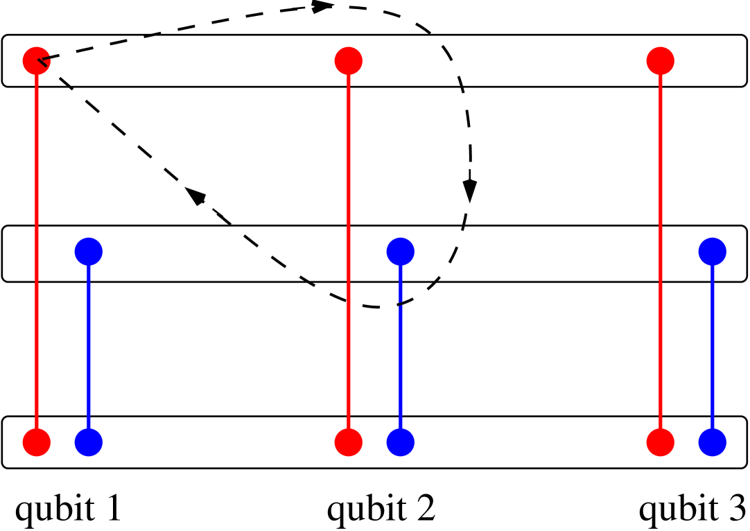
Figure 2: A possible arrangement of anyons comprising a quantum computer. The red particles are the fermions, $X$, while the blue ones can be either $Y$ or $Z$ particles. The depicted evolution results in a controlled phase gate.

The value of the controlled phase gate is fixed by the statistics of the permuted particles and is resilient to any deformations of the spanned loop as long as it circulates the target particles once. Moreover, moving the particles around with the trapping potentials is immune to control errors that would occur if the transportation was performed by dynamical means. For the latter case one has to rotate the effective spins successively along the desired trajectory, with errors that would accumulate at each translation step. By moving the potential well adiabatically the trapped particle follows the lowest energy configuration without the need for any dynamical control of the effective spins and subsequent introduction of control errors. This resilience which is of geometrical origin gives a great advantage in transporting and braiding the anyons fault tolerantly.

It has been shown Duan_02 that Hamiltonian (1) can be generated with a Bose-Einstein condensate of atoms superposed with a two dimensional optical lattice configuration. In particular, consider two bosonic species labelled by $\sigma=a,b$, e.g. given by two hyperfine levels of an atom. They can be trapped by employing two in-phase optical lattices for each direction. The geometry of the hexagonal lattice can be produced with three pairs of properly aligned counterpropagating laser fields Duan_02 . The tunnelling of atoms between neighboring sites is described by $-\sum_{l\sigma}(t_{\sigma}a_{l\sigma}^{\dagger}a_{(l+1)\sigma}+\text{H.c.})$. When two or more atoms are present in the same site, they experience collisions given by ${1\over 2}\sum_{l\sigma\sigma^{\prime}}U_{\sigma\sigma^{\prime}}a^{\dagger}_{l\sigma}a^{\dagger}_{l\sigma^{\prime}}a_{l\sigma^{\prime}}a_{l\sigma}$. We now consider the limit $t\ll U$ where the system is in the Mott insulator regime with one atom per lattice site Raithel . In this regime, we can employ the pseudospin basis of $|\!\!\uparrow\rangle\equiv|n_{l}^{a}=1,n_{l}^{b}=0\rangle$ and $|\!\!\downarrow\rangle\equiv|n_{l}^{a}=0,n_{l}^{b}=1\rangle$, for lattice site $l$, and the effective evolution can be expressed in terms of the corresponding Pauli operators. Consider initially high enough laser intensities such that each site corresponds to a free spin $1/2$ particle. By applying Raman transitions between the states $\left|\,a\right\rangle$ and $\left|\,b\right\rangle$ it is possible to perform an arbitrary local spin rotation. It is easily verified that when one of the tunnelling coupling is activated, say $t_{a}$, the Ising interaction is realized between neighboring sites Pachos1 ; Kuklov ; Duan_02 ,

$$H_{1}=-t_{a}^{2}\Big{(}\frac{1}{U_{aa}}-\frac{1}{2U_{ab}}\Big{)}\sum_{<l,m>}\sigma^{z}_{l}\sigma^{z}_{m},$$ (5)

where $<l,m>$ are the nearest neighbors connected by the $t_{a}$ coupling. This procedure can implement the interactions of the $z$-links of Hamiltonian (1), where the $J_{z}$ coupling varies as a function of $t_{a}$. To generate the interactions in the $x$- and $y$-links one needs to create an anisotropy between the $x$ and $y$ spin directions. For that we activate a tunnelling by means of Raman couplings Pachos1 ; Duan_02 consisting of two standing lasers $L_{1}$ and $L_{2}$, giving finally the interaction terms $\sum_{<l,m>}\sigma^{x}_{l}\sigma^{x}_{m}$ or $\sum_{<l,m>}\sigma^{y}_{l}\sigma^{y}_{m}$ depending on the phase difference between the laser radiations, $L_{1}$ and $L_{2}$. Appropriate combinations of these interactions gives finally all the necessary terms for realizing Kitaev’s Hamiltonian.

Upon this basis we can realize a quantum computational scheme with abelian anyons. As we have seen, the generation of particle excitations involves the rotation of effective spins, or equivalently, rotations of the spins at the $z$-links of the original lattice. In this way initialization of the qubit space is straightforwardly implemented by local Raman transitions. To perform a one-qubit rotation an appropriate detuned laser radiation can be used to induce a local $\sigma^{z}$ rotation. To perform the trapping of the excitations we choose to use localized $\sigma^{z}\sigma^{z}$ interactions that would lower the $J_{\text{eff}}$ coupling, thereby reducing the overall energy of the excitations at a specific plaquette. This can be implemented simply by focusing a laser field in-between the spins of the $z$-link, that will reduce the potential barrier thus increasing the $t_{a}$ tunnelling (see Eqn. (5)). Note, that this laser does not need to have a cross-section smaller than the lattice period, but merely to have a strong effect on the tunnelling between two certain sites and weaker between the rest of the sites, thus trapping the anyonic excitation in that neighborhood. By moving the focus of this laser around the lattice, the potential minimum and its trapped particle will also move accordingly. To suppress the generation of undesired relative phases between the excitations due to fluctuations of the intensity of the trapping laser one can use the same laser source for generating the trapping potentials for all the particles. The main source of decoherence, beyond the leakage of coherence outside the pseudospin space due to heating of the atoms, is the generation of virtual pairs of particles due to thermal fluctuations. These excitations can actually move the particles out of their trapping potentials, which will register as decoherence of the encoded information. To avoid such problems, we would like to have the temperature small enough compared to the depth of the trapping well, $V$, thus exponentially suppressing the generation of virtual pairs.

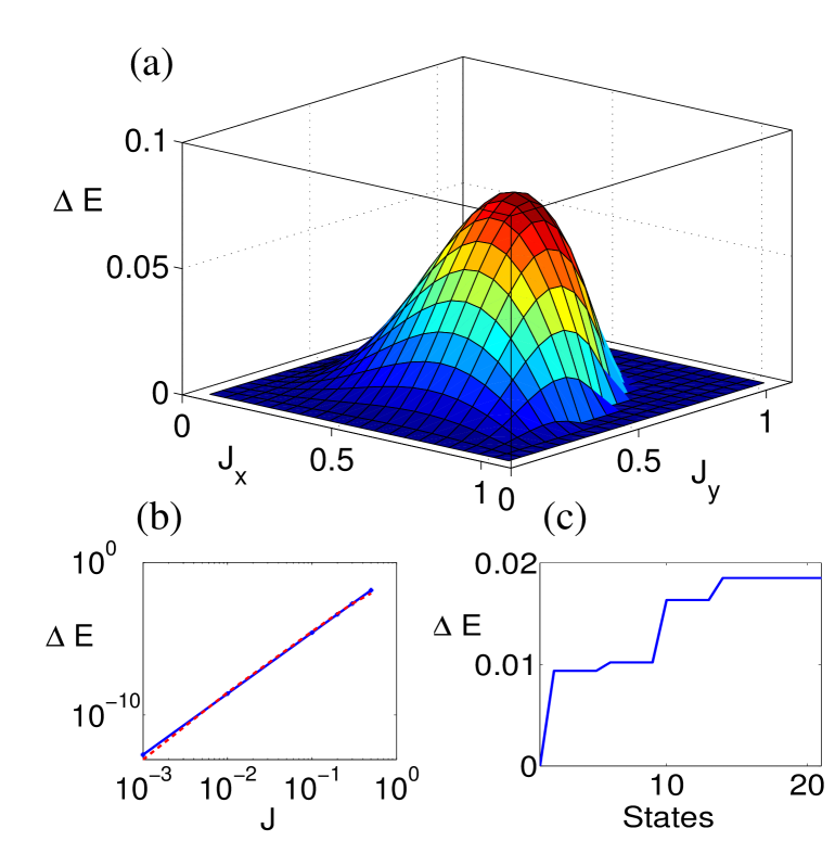
Figure 3: (a) The numerically obtained energy gap, $\Delta E$, between the ground and the first excited state with $J_{z}=1$. (b) Loglog plot of $\Delta E$ as a function of the coupling $J=J_{x}=J_{y}$. There is very good agreement between the solid (blue) line, predicted by perturbation theory, and the dashed (red) line, given by numerical diagonalization. (c) $\Delta E$, for various states above the ground state. As expected from the theory, $\Delta E$ almost doubles for a certain set of states that correspond to $X$ excitations compared to $Y$ or $Z$ excitation.

The measurement procedure required for the presented scheme has to be able to distinguish between the vacuum state and a particular excitation. As we have seen, excitations are localized objects that live within the boundaries of the trapping potentials. A generic measurement should therefore be able to address the density profile of the particular atomic states as a function of position and determine their correlations. To increase the distinguishability between their correlations one may alternatively use local time modulations of the optical lattice to induce Bragg scattering resonant between the particular excitation and the first excited vibrational state of the atoms. By direct population measurement or by measurement of the atomic correlations one can, in principle, deduce the state of the system Toth ; Altman ; Kuklov_99 ; Grondalski .

Finally, we would like to see to which extend perturbation theory describes the initial model by employing numerical diagonalization of Hamiltonian (1). Towards that we consider a periodic honeycomb lattice consisting of 16 spins. Figure 3(a) presents the energy gap, $\Delta E$, between the ground and the first excited states as a function of $J_{x}$ and $J_{y}$ where we have set $J_{z}=1$. It is clear that the model has a gap for $|J_{x}|+|J_{y}|<|J_{z}|$ as expected from the analytical treatment Kitaev . Furthermore, it is possible to compare the energy gap of the perturbative theory with the one obtained numerically for $J_{x},J_{y}\ll J_{z}$. Figure 3(b) presents a comparison between perturbation (solid, blue line) and the numerical diagonalization (dashed, red line) of $\Delta E$ for various values of the coupling $J=J_{x}=J_{y}$. We observe that the two curves are in excellent agreement indicating the validity of perturbation theory for a wide range of coupling values $J$. As a last test we consider a part of the spectrum above the ground state. We saw previously that the energy gap of the fermionic excitation, $X$, is double than the energy gap of $Y$ or $Z$ excitation. Indeed, Figure 3(c) gives $\Delta E$ for the first few excitations where the doubling of $\Delta E$ is clearly observed. Unfortunately, the system of 16 spins that we are able to diagonalize numerically is too small to represent faithfully the properties of the spectrum expected for a large system. A complete theoretical study that presents the properties of the excitation beyond perturbation theory will be presented elsewhere.

Acknowledgements. We would like to thank Alastair Kay, Seth Lloyd, John Preskill and Jörg Schmiedmayer for helpful conversations. This work was supported by the Royal Society.

References

- (1) A. Kitaev, Annals of Physics 303, 2 (2004).
- (2) M. Freedman, M. Larsen, and Z. Wang, Comm. Math. Phys., 227, 605 (2002); M. Freedman, A. Kitaev, M. Larsen, and Z. Wang, Bull. Am. Math. Soc. 40, 31 (2002).
- (3) C. Mochon, Phys. Rev. A 67, 022315 (2003).
- (4) N. Bonesteel, L. Hormozi, G. Zikos, and S. H. Simon, Phys. Rev. Lett. 95, 140503 (2005).
- (5) S. Lloyd, quant-ph/0004010.
- (6) B. Paredes et al., Phys. Rev. Lett. 87, 10402 (2001).
- (7) H. Bombin and M.A. Martin-Delgado, quant-ph/0602063.
- (8) A. Kitaev, cond-mat/0506438.
- (9) J. K. Pachos, to appear in An. of Phys., quant-ph/0605068.
- (10) L.-M. Duan, E. Demler, and M. D. Lukin, Phys. Rev. Lett. 91, 090402 (2003).
- (11) A. Kastberg et al., Phys. Rev. Lett. 74, 1542 (1995); G. Raithel et al., Phys. Rev. Lett. 81, 3615 (1998).
- (12) J. K. Pachos and E. Rico, Phys. Rev. A 70, 053620 (2004).
- (13) A. B. Kuklov and B. V. Svistunov, Phys. Rev. Lett. 90, 100401 (2003).
- (14) G. Toth, Phys. Rev. A 69, 052327 (2004).
- (15) E. Altman, E. Demler, and M. D. Lukin, Phys. Rev. A 70, 013603 (2004).
- (16) A. B. Kuklov, and B. V. Svistunov, Phys. Rev. A 60, R769 (1999).
- (17) J. Grondalski, P. M. Alsingy, and I. H. Deutsch, Optics Express 5, 249 (1999); S. Salma et al., quant-ph/0511258.