Distortion operator and Entanglement Information Rate Distortion of Quantum Gaussian Source

Abstract

Quantum random variable, distortion operator are introduced based on canonical operators. As the lower bound of rate distortion, the entanglement information rate distortion is achieved by Gaussian map for Gaussian source. General Gaussian maps are further reduced to unitary transformations and additive noises from the physical meaning of distortion. The entanglement information rate distortion function then are calculated for one mode Gaussian source. The rate distortion is accessible at zero distortion point. For pure state, the rate distortion function is always zero. In contrast to the distortion defined via fidelity, our definition of the distortion makes it possible to calculate the entanglement information rate distortion function for Gaussian source.

Distortion operator: Two major parts in classical information theory are channel capacity and rate distortion theory. They concern respectively with the reliability and effectiveness of information transmission. In quantum information theory, channel capacity has been widely investigated, but little effort has been put into developing quantum rate-distortion theory[1][2]. It was proven [1] that the quantum rate-distortion function $R(D)$ is lower bounded by entanglement information rate-distortion function $R^{I}(D).$ For a given source $R^{I}(D)$ is defined by

$$R^{I}(D)=\min_{\mathcal{E}\left|d(\mathcal{E)\leq D}\right.}I_{c}(\rho,\mathcal{E}).$$ (1)

where $d$ is some distortion function, and $\mathcal{E}$ is the channel. The result is proven under the assumption of distortion function defined by transmission fidelity. It is linear among different modes. We can extend the distortion function to a more general form. The result will also be true if it is linear among different modes. One of the useful distortion function is mean square function as used in classical information theory for Gaussian source. The mean square distortion in classical theory is $\overline{d}=E(d(Y,Y^{\prime}))=\int p(y,y^{\prime})d(y,y^{\prime})dydy^{\prime}$, with $d(y,y^{\prime})=(y-y^{\prime})^{2}.$ Where $Y$ is the input random variable and $Y^{\prime}$ is the output, $p(y,y^{\prime})$ is the joint density distribution function. The same idea should be extended to quantum information theory. What is the quantum corresponding of random variable? We prefer the canonical operators $X$ and $P$. Then the distortion operator will be introduced as

$$d(A,B)=\frac{1}{2}\sum_{i=1}^{n}[(X_{Ai}-X_{Bi})^{2}+(P_{Ai}+P_{Bi})^{2}].$$ (2)

Where $A$ is the sender and $B$ is the receiver. The Schmidt purification of the sender state $\rho_{A}$ is obtained by introducing the reference system, described by Hilbert space $\mathcal{H}_{R}$, isomorphic to the Hilbert space $\mathcal{H}_{Q}=\mathcal{H}_{A}$ of the initial system, Then there exists a purification of the state $\rho_{A},$ a unit vector $\left|\psi\right\rangle\in\mathcal{H}_{Q}\otimes\mathcal{H}_{R}$ such that $\rho_{A}=Tr_{R}\left|\psi\right\rangle\left\langle\psi\right|.$Where$\left|\psi\right\rangle=\sum_{k}\sqrt{\lambda_{k}}\left|\lambda_{k}\right\rangle\left|\lambda_{k}\right\rangle$, with $\lambda_{k}$ and $\left|\lambda_{k}\right\rangle$ are eigenvalue and eigenvector of $\rho_{A}$ respectively. After transmission, the joint state will be $\rho^{RQ^{\prime}}=(\mathcal{E}\otimes\mathbf{I})\left|\psi\right\rangle\left\langle\psi\right|,$ it is easy to verify that $\rho_{A}=Tr_{Q}(\rho^{RQ^{\prime}})$ and $\rho_{B}=Tr_{R}(\rho^{RQ^{\prime}})=\mathcal{E}(\rho_{A}),$ which means the system $R$ remains at the input state $\rho_{A}$ and system $Q$ evolves to the output state $\rho_{B}.$ The average distortion will be

$$\overline{d}=Tr\rho^{RQ^{\prime}}d(A,B).$$ (3)

A similar quantity was introduced to obtain entanglement of formation of symmetric Gaussian states [3]. The average distortion possesses some kind of EPR-uncertainty of the joint state, we here neglect the mean of canonical operators for simplicity, thus all of the first moments of the states will be neglected in the follows.

Entanglement information rate-distortion function: The coherent information $I_{c}(\rho,\mathcal{E})=S(\mathcal{E}(\rho))-S(\rho^{RQ^{\prime}}).$ The Entanglement information rate-distortion function is the global minimum of the coherent information under the certain distortion. There is a useful lemma in classical information theory which gives necessary and sufficient conditions for the global minimum of a convex function of probability distributions in terms of the first partial derivatives. The lemma was extended to quantum information theory [4] in evaluating the capacities of bosonic Gaussian channels. Let $F$ be a convex function on the set of density operators which contains $\rho_{0}$ and $\rho,$ the necessary and sufficient condition for $F$ achieves minimum on $\rho_{0}$ is that the convex function $F((1-t)\rho_{0}+t\rho)$ of the real variable $t$ achieves minimum at $t=0$ for any $\rho.$ That is $\frac{d}{dt}\left|{}_{t=0}F((1-t)\rho_{0}+t\rho)\geq 0\right..$ Here $I_{c}(\rho,\mathcal{E})$ is a function of density operator $\rho^{RQ^{\prime}}.$ Coherent information is convex due to channel operation[1], that is for operation $\mathcal{E}_{\lambda}\equiv\lambda\mathcal{E}_{1}\mathcal{+}(1-\lambda)\mathcal{E}_{2},$ where $0\leq\lambda\leq 1,$ one has $I_{c}(\rho,\mathcal{E}_{\lambda})\leq\lambda I_{c}(\rho,\mathcal{E}_{1})+(1-\lambda)I_{c}(\rho,\mathcal{E}_{2})$. Thus coherent information is a convex function of density operator $\rho^{RQ^{\prime}}.$ Suppose the minimum is achieved at $\rho_{0}^{RQ^{\prime}}=(\mathcal{E}_{0}\otimes I)\left|\psi\right\rangle\left\langle\psi\right|,$ the necessary and sufficient condition will be

$$\frac{d}{dt}\left|{}_{t=0}I_{c}(\rho,(1-t)\mathcal{E}_{0}+t\mathcal{E})\geq 0\right..$$ (4)

The derivative will be$-Tr(\mathcal{E}(\rho)\mathcal{-E}_{0}(\rho))\log\mathcal{E}_{0}(\rho)+Tr(\rho^{RQ^{\prime}}-\rho_{0}^{RQ^{\prime}})\log\rho_{0}^{RQ^{\prime}}.$ If $\mathcal{E}_{0}$ is a trace preserving completely positive (CP) Gaussian operation, then for a Gaussian input state $\rho$, the output state $\mathcal{E}_{0}(\rho)$ and the joint state $\rho_{0}^{RQ^{\prime}}$ will be Gaussian. Hence their logarithms are quadratic polynomials in the corresponding canonical variables[4]. The derivative will be zero under the constrains of the first and second moments. Where the trace preserving property of $\mathcal{E}$ is also used. The conclusion is that for any channels with the same first and second moments, Gaussian channel achieves the minimum of coherent information. The moments of the channel is with respect to a given Gaussian input state.

Gaussian channel: Gaussian CP maps are defined as maps which transform Gaussian states into Gaussian states. Gaussian CP map is thus isomorphic to bipartite Gaussian state[5][6]

$$G=\int_{\mathbb{R}^{4n}}dx\exp(-\frac{1}{4}x^{T}\Gamma x+iD^{T}x-C)W(x),$$ (5)

where $W(x)=\exp[-ix^{T}R]$ are Weyl operators and $R=(X_{1},P_{1},X_{2},\cdots,P_{2n}),$ with $[X_{k},P_{l}]=i\delta_{kl}$.We in the following will omitted the linear part $D^{T}$ and the constant $C$ which are not critical in our problem. The output state will be $\mathcal{E}(\rho)\propto Tr_{2}[G^{T_{2}}\rho],$where the trace is taking on the second part of $G^{T_{2}}$ and the input state $\rho$. The completely positive map on the input state will be $\rho^{RQ^{\prime}}=(\mathcal{E}\otimes\mathbf{I)(}\left|\psi\right\rangle\left\langle\psi\right|\mathbf{).}$ The correlation matrix (CM) of the Schmidt purification $\left|\psi\right\rangle$ is [4]

$$\gamma_{\psi}=\left[\begin{array}[]{ll}\gamma&\beta\\ \beta^{T}&\gamma\end{array}\right],$$

where $\gamma$ is the CM of input state $\rho$, $\beta=-\beta^{T}=J_{n}\sqrt{-(J_{n}^{-1}\gamma)^{2}-\mathbf{I}}$ are purely off-diagonal, where

$$J_{n}=\bigoplus_{k=1}^{n}J,\text{ }J=\left[\begin{array}[]{ll}0&-1\\ 1&0\end{array}\right]$$

Every operators $A\in\mathcal{B}\mathcal{(H)}$ is completely determined by its characteristic function $\chi_{A}(x):=Tr[AW(x)]$ [7]. It follows that $A$ may be written in terms of $\chi_{A}$ as[8] $A=\pi^{-m}\int_{\mathbb{R}^{m}}dx\chi_{A}(x)W(-x).$ Thus$\left|\psi\right\rangle\left\langle\psi\right|=\pi^{-4n}\int_{\mathbb{R}^{4n}}dx\chi_{\psi}(x)W(-x),$ with $\chi_{\psi}(x)=\exp[-\frac{1}{4}x^{T}\gamma_{\psi}x]$, we assume the first moments of the input state $\rho$ be zero. Hence $\rho^{RQ^{\prime}}\mathbf{=}\pi^{-4n}\int_{\mathbb{R}^{4n}}dx_{1}dx_{2}\chi_{\psi}(x_{1},x_{2})W(-x_{2})Tr_{2}[G^{T_{2}}W(-x_{1})]$The CM of $\rho^{RQ^{\prime}}$ will be

$$\left[\begin{array}[]{ll}\widetilde{\Gamma}_{1}-\widetilde{\Gamma}_{12}(\widetilde{\Gamma}_{2}+\gamma)^{-1}\widetilde{\Gamma}_{12}^{T}&\widetilde{\Gamma}_{12}(\widetilde{\Gamma}_{2}+\gamma)^{-1}\beta\\ \beta^{T}(\widetilde{\Gamma}_{2}+\gamma)^{-1}\widetilde{\Gamma}_{12}^{T}&\gamma-\beta^{T}(\widetilde{\Gamma}_{2}+\gamma)^{-1}\beta\end{array}\right].$$ (6)

Where we have denoted

$$\Gamma=\left[\begin{array}[]{ll}\Gamma_{1}&\Gamma_{12}\\ \Gamma_{12}^{T}&\Gamma_{2}\end{array}\right],$$

and $\widetilde{\Gamma}=(\mathbf{I\oplus}\Lambda)\Gamma(\mathbf{I\oplus}\Lambda)$, with $\Lambda=diag(1,-1,1,-1,\cdots,1,-1)$ is a diagonal matrix which represents the transposition in phase space $(X_{j}\rightarrow X_{j},P_{j}\rightarrow-P_{j}).$The CM of the out output state $\mathcal{E}(\rho)$ is $\gamma^{\prime}=\widetilde{\Gamma}_{1}-\widetilde{\Gamma}_{12}(\widetilde{\Gamma}_{2}+\gamma)^{-1}\widetilde{\Gamma}_{12}^{T}$. Now we turn to the trace-preserving Gaussian CP maps[9] which describe all actions that can be performed on $\rho$ by first adding ancillary systems in Gaussian states, then performing unitary Gaussian transformations on the whole system, and finally discarding the ancillas. On the level of CMs these operations were shown to be described by $\gamma\mapsto\gamma^{\prime}=M^{T}\gamma M+N.$ The Gaussian operator that corresponds to this operation has the CM[5]

$$\Gamma=\lim_{r\rightarrow\infty}\left[\begin{array}[]{ll}M^{T}A_{r}M+N&M^{T}C_{r}\\ C_{r}M&A_{r}\end{array}\right],$$

where $A_{r}=\cosh r\mathbf{I}$ and $C_{r}=\sinh r\Lambda$. By taking the limitation of $r\rightarrow\infty$ one has the CM of $\rho^{RQ^{\prime}}$ to be

$$\Gamma^{\prime}=\left[\begin{array}[]{ll}\Gamma_{1}^{\prime}&\Gamma_{12}^{\prime}\\ \Gamma_{12}^{\prime T}&\Gamma_{2}^{\prime}\end{array}\right]=\left[\begin{array}[]{ll}M^{T}\gamma M+N&M^{T}\beta\\ \beta^{T}M&\gamma\end{array}\right].$$ (7)

This is the final result for a trace-preserving Gaussian map on an input Gaussian state. The reason that we restrict ourself to the trace-preserving Gaussian CP maps is from the physical consideration. The result state of trace-preserving Gaussian CP map is a state with its CM $\gamma$ remains intact in the reference system $R$ (see Eq.(7)), hence we can compare the output of the $Q$ system with the input state which is keep intact in $R$ system. While a general Gaussian CP map will not only change the $Q$ system but also the reference system $R$ (see Eq.(6)). The distortion is some kind of difference between the output and the input. If the input state can not keep, the definition of the distortion will lost its basis. Hence we can only define distortion on the basis of trace-preserving Gaussian CP maps with a clearly physical meaning.

One mode Gaussian state: The positivity of $\rho^{RQ^{\prime}}$can be written as the uncertainty relation $\Gamma^{\prime}-iJ_{12,n}\geq 0.$ Due to our selection of the purely off-diagonal $\beta$, we have $J_{12,n}=J_{n}\oplus(-J_{n}).$ For a one mode Gaussian state input, $\Gamma^{\prime}$ is a $4\times 4$ matrix. The uncertainty relation requires $\det(\Gamma^{\prime}-iJ_{12})\geq 0$ which can be expressed as[10]

$$\det\Gamma_{1}^{\prime}\det\Gamma_{2}^{\prime}-\det\Gamma_{1}^{\prime}-\det\Gamma_{2}^{\prime}+(1+\det\Gamma_{12}^{\prime})^{2}-Tr(J\Gamma_{1}^{\prime}J\Gamma_{12}^{\prime}J\Gamma_{2}^{\prime}J\Gamma_{12}^{\prime T})\geq 0.$$

The sign before $\det\Gamma_{12}^{\prime}$ now is positive due to $J_{12}=J\oplus(-J).$ Denote $K=\det M,$ and $N=M^{T}N^{\prime}M,$ the inequality will reduced to $K^{2}\det N^{\prime}-(1-K)^{2}\geq 0,$ that is

$$\det N-(1-K)^{2}\geq 0,$$ (8)

where we have used $\det(A+B)=\det A+\det B-Tr(JAJB),$ $M^{T}JM=K$ and $\det\gamma_{\psi}=1.$ One the other hand, the positivity of the output state reads $\Gamma_{1}^{\prime}-iJ\geq 0,$ thus $M^{T}\gamma M+N-iJ=M^{T}(\gamma-iJ)M+N-iJ(1-K)\geq 0.$ For any input state we have $\gamma-iJ\geq 0,$ the equality can be achieved by pure state, hence we have $N-iJ(1-K)\geq 0$ which will also lead to Ineq.(8).

The physical meaning of Gaussian trace-preserving map indicated by $M$ and $N$ is that $N$ is the additive noise and $M$ is a symplectic transformation (rotation and squeezing) and a successively amplitude damping or amplification. Let us consider the amplitude damping (as well as amplification) of the channel, which is described by $\det(M)=K.$ The amplitude of the signal is damped by a factor of $k=\sqrt{K}$, what will we do to retrieve the input, clearly we will amplify it back. Or we will reduce the input state with the same factor to compare with the output. In these two cases, the distortion operators will be modified to $d(A,B)=\frac{1}{2}[(X_{A}/k-X_{B})^{2}+(P_{A}/k+kP_{B})^{2}]$ and $d(A,B)=\frac{1}{2}[(X_{A}-kX_{B})^{2}+(P_{A}+kP_{B})^{2}]$ respectively. In both these situations, if we take all the steps as a whole channel, then we have $K=1.$ Hence in the following we just need to consider the channel of symplectic transformation and additive noise.

Let us consider the coherent information, which is determined by the symplectic eigenvalues of $\Gamma^{\prime}$ and $\Gamma_{1}^{\prime}.$ Now $\det M=1,$ hence $(M\oplus\mathbf{I})$ are symplectic transformations, which preserve the symplectic eigenvalues so that the coherent information. $\Gamma^{\prime}$ can be written as $\Gamma^{\prime}=(M^{T}\oplus\mathbf{I})\Gamma^{\prime\prime}(M\oplus\mathbf{I})$, with $\Gamma_{1}^{\prime\prime}=\gamma+\left(M^{T}\right)^{-1}NM^{-1},$ $\Gamma_{12}^{\prime\prime}=\beta,\Gamma_{2}^{\prime\prime}=\gamma$ correspondingly.

The problem is to search a $M$ such that the average distortion $\overline{d}$ is minimized. We have

$$\overline{d}=\frac{1}{4}[TrN+TrM^{T}\gamma M+Tr\gamma-2TrM\beta\Lambda].$$ (9)

The minimization of $\overline{d}$ will involve algebra equation of power $4.$ Let us firstly consider the input of the thermal state whose CM is $\gamma_{s}\mathbf{I,}$ with $\gamma_{s}=2N_{s}+1$ is the symlectic eigenvalue of the CM $\gamma$ and $N_{s}$ is the average photon number of the state. Denote $\frac{1}{4}TrN=N_{n}$, we have

$$M=\left[\begin{array}[]{ll}\sqrt{1+s^{2}-\delta^{2}}&s+\kappa\\ s-\kappa&\sqrt{1+s^{2}-\delta^{2}}\end{array}\right],$$

with $s=\sqrt{\gamma_{s}^{2}-1}/(2\gamma_{s})\equiv\sinh r_{s}$, and the distortion operator

$$\overline{d}=\frac{1}{4}(\frac{1}{\gamma_{s}}+3\gamma_{s})+N_{n}.$$

The minimal $N_{n}$ is $0,$ hence the minimal $\overline{d}_{\min}=\frac{1}{4}(\frac{1}{\gamma_{s}}+3\gamma_{s}),$ thus we define a canonical distortion $\overline{d}_{c}$ instead of $\overline{d}$, $\overline{d}_{c}=\overline{d}-\overline{d}_{\min},$

$$\overline{d}_{c}=N_{n}.$$ (10)

The coherent information now is determined by the symplectic eigenvalues of $\Gamma^{\prime\prime}$ and $\Gamma_{1}^{\prime\prime}$ . The symplectic eigenvalues are functions of the trace and determinant of the noise term $\left(M^{T}\right)^{-1}NM^{-1}.$ Denote $\delta=\frac{1}{4}\det N,$ $\tau=\frac{1}{2}Tr[\left(M^{T}\right)^{-1}NM^{-1}],$ the coherent information of the state with CM$\;\Gamma^{\prime\prime}$ will be [11][4]

$$I_{c}=g(d_{0}-\frac{1}{2})-g(d_{1}-\frac{1}{2})-g(d_{2}-\frac{1}{2}).$$ (11)

Where $g(x)=(x+1)\log(x+1)-x\log(x)$ is the bosonic entropy function, and $d_{0}^{2}=x+(N_{s}+\frac{1}{2})^{2},$ $d_{1,2}^{2}=\frac{1}{2}[x+\frac{1}{2}\pm\sqrt{x^{2}-4N_{s}(N_{s}+1)\delta}],$ with $x=\delta+(N_{s}+\frac{1}{2})\tau.$ The entanglement information rate distortion $R^{I}$ now is the minimization of $I_{c}$ over all possible noise matrix $N$ with given trace $TrN=4N_{n}.$ After the determinant and the trace of the noise matrix $N$ are given, we still have the freedom in choosing the off-diagonal elements or the difference of the diagonal elements. This freedom and the undetermined parameter $\kappa$ in the matrix $M$ are combined into a parameter $t$ ($-1\leq t\leq 1$) and we can express $\tau$ as $\tau=2[N_{n}\cosh(2r_{s})+t\sqrt{N_{n}^{2}-\delta}\sinh(2r_{s})].$ Thus

$$R^{I}=\min_{\delta,t}I_{c}(x(\delta,t),\delta).$$

The minimization will be achieved when $\delta=N_{n}^{2},$ we prove this by firstly preserving $x$ while increases $\delta.$ When $\sinh(2r_{s})\geq N_{n}/2,$ this is always possible by varying $t$ properly to compensate the change of $x$ caused by the increase of $\delta$. We have $\frac{\partial I_{c}(x,\delta)}{\partial\delta}=c_{0}[f(d_{1}-\frac{1}{2})-f(d_{2}-\frac{1}{2})].$ where $f(a)=\frac{1}{2a+1}\log\frac{a+1}{a}$ is a monotonically decreasing function and $c_{0}=\frac{x}{\sqrt{x^{2}-4N_{s}(N_{s}+1)\delta}}>0.$ Thus $\frac{\partial I_{c}(x,\delta)}{\partial\delta}\leq 0,$ $I_{c}(x,\delta)$ monotonically decreases with $\delta$ increases while preserving $x.$ The minimum is achieved at $\delta=N_{n}^{2}$, that is, the noise matrix $N$ is proportional to the unity matrix. The condition $\sinh(2r_{s})\geq N_{n}/2$ may contain most of the situations. For most of the input states (i.e. $N_{s}>0.012$) when $N_{n}=2\sinh(2r_{s}),$ the values of the coherent information will be $0$ at $\delta=N_{n}^{2}$. We need further to consider the situation of weak signal input states (i.e. $N_{s}\leq 0.01$). There is the case that $x(0,t)$ is too small compared with $x(N_{n}^{2},t)$ for all $t.$ So we need firstly increase $x$ from $x(0,t_{0})$ to some intermediate state with $x(\delta_{1},t_{1})=x(N_{n}^{2},t)$ while in the $x$ increasing process the coherent information is decreased. Let $x_{1,2}=\frac{1}{2}[x^{2}\pm 4N_{s}(N_{s}+1)\delta]$, we increases $x$ and $\delta$ while keeping $x_{2}$ invariant, then $\frac{\partial I_{c}(x_{1},x_{2})}{\partial x_{1}}=\frac{1}{x}[f(d_{0}-\frac{1}{2})-\frac{1}{2}(f(d_{2}-\frac{1}{2})+f(d_{2}-\frac{1}{2}))].$ The function $f$ is not only a monotonically decreasing but also a downward convex function. Hence in order to prove $\frac{\partial I_{c}(x_{1},x_{2})}{\partial x_{1}}\leq 0,$ we only need to prove $d_{0}\geq\frac{1}{2}(d_{1}+d_{2})$ which is confirmed by the fact that $d_{0}^{2}-\frac{1}{2}(d_{1}^{2}+d_{2}^{2})$ $=$ $(N_{s}+\frac{1}{2})^{2}+\frac{1}{2}x-\frac{1}{4}=N_{s}(N_{s}+1)+\frac{1}{2}x>0.$ This completes our proof. The entanglement information rate distortion of thermal state input as a function of the canonical distortion $N_{n}$ will be

$$R^{I}(N_{n})=\max\{0,I_{c}(\delta=N_{n}^{2},\tau=2N_{n}\cosh(2r_{s}))\}.$$ (12)

where $\cosh(2r_{s})=1+2N_{s}(N_{s}+1)/(2N_{s}+1)^{2}.$

For the general input $\gamma,$ we may further transform the CM $\Gamma^{\prime\prime}$ to $\Gamma^{\prime\prime\prime}$ by symplectic transformation $S\oplus S,$ $S$ diagonalizes $\gamma$ by $S^{T}\gamma S=\gamma_{s}\mathbf{I}$, with $\gamma_{s}$ is the symplectic eigenvalue. Thus $\Gamma^{\prime\prime\prime}$ will be a CM with its submatrices are $\Gamma_{1}^{\prime\prime\prime}=\gamma_{s}\mathbf{I}+S^{T}\left(M^{T}\right)^{-1}NM^{-1}S,$ $\Gamma_{12}^{\prime\prime\prime}=\beta,\Gamma_{2}^{\prime\prime\prime}=\gamma_{s}\mathbf{I}$ correspondingly. $M$ is determined by the minimization of $\overline{d}$. The above proving that minimization of coherent information is achieved at $\delta=N_{n}^{2}$ remains true for general input $\gamma$. The only difference is that we now have $\tau=[N_{n}\Omega+t\sqrt{N_{n}^{2}-\delta}\sqrt{\Omega^{2}-4}],$ where $\Omega=\sum_{i,j=1}^{2}M_{ij}^{\prime 2},$ $M^{\prime}=S^{-1}M.$ We have $\Omega=\frac{1}{\gamma_{s}}TrM^{T}\gamma M$ to be the function of trace and determinant of the input CM $\gamma$. The entanglement information rate distortion will be

$$R^{I}(N_{n})=\max\{0,I_{c}(\delta=N_{n}^{2},\tau=N_{n}\Omega)\}.$$ (13)

A special case is the pure state input which contains squeezed states (for coherent states and squeezed coherent states the distortion operator should be modified). We have $\Omega=2$ which is the minimal of $\Omega.$ Thus $R^{I}(N_{n})=\max\{0,g(N_{s}+N_{n})-g(N_{sn1})-g(N_{sn2})\},$where $N_{sn1,2}=\frac{1}{2}(\sqrt{(N_{n}+1)^{2}+4N_{n}N_{s}}-1\pm N_{n}).$ Because $N_{s}=0$ so that $R^{I}(N_{n})\equiv 0$ for pure states.

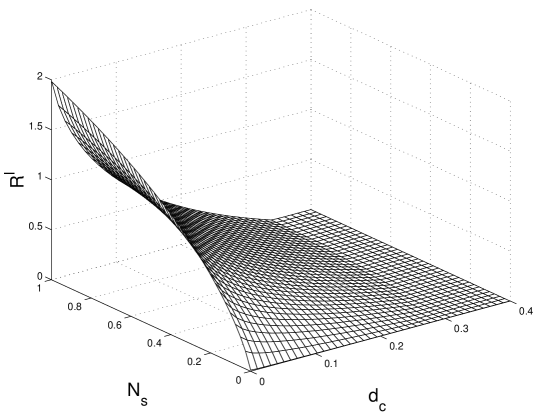
Figure 1: Entanglement information rate distortion, the trace of input CM is $Tr\gamma=3,N_{s}=0$ for pure state, the maximal $N_{s}$ is for thermal state input.

Conclusions and Discussions: We proposed the distortion operator which is quadratic of the canonical operators. The distortion operator has a good classical correspondence of mean square error. The distortion is the trace of the distortion operator on the joint state density operator. It is an extension of the definition of classical distortion. For quantum Guassian state source, we proved that the entanglement information rate distortion which is a lower bound of the rate distortion is achieved by Gaussian map under the constrain of zeroth, first and second moments. In the language of distortion operator, distortion defined with fidelity ($1-F_{e}$) corresponds to the distortion operator of $\mathbf{I-}\left|\Psi\right\rangle\left\langle\Psi\right|,$ where $\left|\Psi\right\rangle$ is the purification of the source state. The quadratic canonical operator distortion is more convenient than fidelity distortion for Gaussian state.

By the physical meaning of the distortion, we rule out the non-trace-preserving Gaussian maps and convert the amplitude damping or amplification channels to the standard maps which contain a symplectic transformation and an additive noise in the language of correlation matrix. For one-mode Gaussian state input, we proved that the entanglement information rate distortion is achieved when the additive noise matrix is proportional to unity matrix. The canonical distortion is simply the average photon number of the noise. The rate distortion for pure state input is zero.

One of the most important conclusion we can draw is that the rate distortion function is accessible for noiseless case. For any one mode Gaussian input states, the entanglement information rate distortion functions at the point of zero distortion are $R^{I}(0)=g(N_{s}),$ which is the entropy of the source $S(\rho).$ From Schumacher’s quantum noiseless coding theorem[12] we know that $R(0)=S(\rho).$ Thus we have the conclusion that $R(0)=R^{I}(0).$

Acknowledgement: Funding by the National Natural Science Foundation of China (under Grant No. 10575092), Zhejiang Province Natural Science Foundation (Fund for Talented Professionals, under Grant No. RC104265) and AQSIQ of China (under Grant No. 2004QK38) are gratefully acknowledged.

References

• [1] H. Barnum, Quantum rate-distortion coding, Phys. Rev. A 62, 42309(2000).
• [2] I. Devetak and T. Berger, Quantum rate-distortion theory for memoryless sources. IEEE Transactions on Information Theory 48(6): 1580-1589 (2002).
• [3] G. Giedke, M. M. Wolf, O. KrΓΌger, R. F. Werner, and J. I. Cirac ,Phys. Rev. Lett.Β 91, 107901 (2003).
• [4] A. S. Holevo and R. F. Werner, Phys.Rev. A 63, 032312 (2001).
• [5] G. Giedke and J. I. Cirac, Phys. Rev. AΒ 66, 032316 (2002).
• [6] J. FiurΓ‘Ε‘ek, Phys. Rev. Lett. 89, 137904 (2002)
• [7] D. Petz, An Invitation to the Algebra of Canonical Commutation Relations, Leuven University Press, Leuven (1990).
• [8] A. Perelomov, Generalized Coherent states, Springer Verlag, Berlin (1986).
• [9] B. Demoen, P.Vanheuverzwijn, and A. Verbeure, Lett. Math. Phys. 2, 161 (1977).
• [10] R. Simon, Phys. Rev. Lett. 84, 2726 (2000).
• [11] X. Y. Chen and P. L. Qiu, Chin. Phys. 10, 779 (2001).
• [12] B. Schumacher, Phys. Rev. AΒ 51, 2738 (1995).