All Inequalities for the Relative Entropy

Abstract

The relative entropy of two $n$-party quantum states is an important quantity exhibiting, for example, the extent to which the two states are different. The relative entropy of the states formed by reducing two $n$-party to a smaller number $m$ of parties is always less than or equal to the relative entropy of the two original $n$-party states. This is the monotonicity of relative entropy.

Using techniques from convex geometry, we prove that monotonicity under restrictions is the only general inequality satisfied by relative entropies. In doing so we make a connection to secret sharing schemes with general access structures.

A suprising outcome is that the structure of allowed relative entropy values of subsets of multiparty states is much simpler than the structure of allowed entropy values. And the structure of allowed relative entropy values (unlike that of entropies) is the same for classical probability distributions and quantum states.

I Entropy and relative entropy

Entropy inequalities play a central role in information theory Cover:Thomas , classical or quantum. This is so because practically all capacity theorems are formulated in terms of entropy, and the same, albeit to a lesser degree, holds for many monotones, of, for example, entanglement: e.g., the entanglement of formation BDSW or squashed entanglement CW:04 . It may thus come as a surprise that until recently LW05 essentially the only inequality known for the von Neumann entropies in a composite system is strong subadditivity

$$S(\rho^{AB})+S(\rho^{BC})\geq S(\rho^{ABC})+S(\rho^{B}),$$ (1)

proved by Lieb and Ruskai LR73 . We use the notation $\rho^{ABC}$ for the density operator representing the state of the system $ABC$, with the notation $\rho^{BC}=\operatorname{Tr}_{A}\rho^{ABC}$ etc. for the reduced states.

The relative entropy of two states $\rho,\sigma$ (density operators of trace $1$) is defined as

$$D(\rho\|\sigma)=\begin{cases}\operatorname{Tr}\rho(\log\rho-\log\sigma)&\text{ if }\operatorname{supp}\,\rho\subset\operatorname{supp}\,\sigma,\\ +\infty&\text{ otherwise},\end{cases}$$

where $\operatorname{supp}\,\rho$ is the supporting subspace of the density operator $\rho$. Note that in this paper, log always denotes the logarithm to base 2. Like von Neumann entropy, the relative entropy is used extensively in quantum information and entanglement theory to obtain capacity-like quantities and monotones. The most prominent example may be the relative entropy of entanglement VedPlen ; VPRK . Many other applications of the relative entropy are illustrated in the review Vedral .

In this paper we study the universal relations between the relative entropies in a composite system and for general pairs of states. For the most part we shall restrict ourselves to finite dimensional spaces.

What are the known inequalities? First of all, the relative entropy is always nonnegative, and indeed $0$ iff $\rho=\sigma$ (see the recent survey by Petz Petz ). The most important, and indeed only known inequality, for the relative entropy is the monotonicity,

$$D(\rho^{AB}\|\sigma^{AB})\geq D(\rho^{A}\|\sigma^{A})$$ (2)

for a bipartite system $AB$. This relation can be derived from strong subbadditivity, eq. (1), as was shown by Lindblad Lindblad in the finite dimensional case; Uhlmann Uhlmann later showed it in generality. To illustrate the connection, strong subadditivity can be easily derived from eq. (2). Note that we can identify the following relative entropy quantity with quantum mutual information CA:97 :

$$D(\rho^{AB}\|\rho^{A}\otimes\rho^{B}) =\operatorname{Tr}{\big{(}\rho^{AB}\log\rho^{AB}\big{)}}-\operatorname{Tr}{\big{(}\rho^{AB}\log(\rho^{A}\otimes\rho^{B})\big{)}}$$

$$=-S(\rho^{AB})-\operatorname{Tr}{\big{(}\rho^{AB}\log\rho^{A}\big{)}}-\operatorname{Tr}{\big{(}\rho^{AB}\log\rho^{B}\big{)}}$$

$$=-S(\rho^{AB})+S(\rho^{A})+S(\rho^{B})$$

$$=I(A\mathrel{\mathop{\mathchar 58\relax}}B).$$

Hence we can recover strong subadditivity from the monotonicity relation

$$D(\rho^{ABC}\|\rho^{AB}\otimes\rho^{C})\geq D(\rho^{BC}\|\rho^{B}\otimes\rho^{C}),$$

as follows:

$$0 \leq D(\rho^{ABC}\|\rho^{AB}\otimes\rho^{C})-D(\rho^{BC}\|\rho^{B}\otimes\rho^{C})$$

$$=I(AB\mathrel{\mathop{\mathchar 58\relax}}C)-I(B\mathrel{\mathop{\mathchar 58\relax}}C)$$

$$=S(\rho^{AB})+S(\rho^{C})-S(\rho^{ABC})-S(\rho^{B})-S(\rho^{C})+S(\rho^{BC})$$

$$=S(\rho^{AB})+S(\rho^{BC})-S(\rho^{ABC})-S(\rho^{B}).$$

Before returning to relative entropy we make a few further observations about entropy. For an $n$-party system, there are $2^{n}-1$ non-trivial reduced states, with their entropies, so we can associate with each state a vector of $2^{n}-1$ real coordinates. Pippenger Pippenger , following the programme of Yeung and Zhang in the classical case Yeung , showed that, after going to the topological closure, the set of all entropy vectors is a convex cone. Hence it must be describable by linear (entropy) inequalities, like strong subadditivity, and one can ask if the entropy cone coincides with the cone defined by the ”known” inequalities (strong subadditivity in the quantum case, additionally positivity of conditional entropy classically). This is indeed the case for $n\leq 3$: the classical result is due to Yeung and Zhang Yeung , the quantum case by Pippenger Pippenger . Yeung and Zhang YZ have however found a new, ”non-Shannon type” inequality for $n=4$ classical parties, and Linden and Winter LW05 found a new so-called constrained inequality for $n=4$ quantum parties, providing evidence that to describe the entropy cones of four and more parties one needs new inequalities, too.

In LW05 Linden and Winter describe how the putative vector of entropies,

$$[S_{A},S_{B},\ldots,S_{ABCD}]=\lambda[3,3,2,2,4,3,3,3,3,4,4,4,3,3,2],$$ (3)

for $\lambda\geq 0$, satisfies strong subadditivity for all subsets of parties $ABCD$, but is nonetheless not achievable by any quantum state $\rho$ [i.e. there is no quantum state $\rho$ such that $S_{A}=S_{A}(\rho_{A}),S_{B}=S_{B}(\rho_{B})$ etc. achieving the values in eq. (3)]. Here we ask (and answer in the affirmative) the question of whether any vector

$$[D_{A},D_{B},\ldots,D_{ABCD}]$$

in which the numbers $D_{A},\ldots,D_{ABCD}$ satisfy the constraints of monotonicity for all subgroups may be realised as the relative entropy of pairs of states [i.e. for any such vector we show that there are states $\rho$ and $\sigma$ such that $D_{A}=D(\rho_{A}\|\sigma_{A})$ etc.]

In this paper we prove the result that for relative entropy, monotonicity is necessary and sufficient to describe the complete set of realisable relative entropy vectors. This is a surprising discovery as relative entropy is a seemingly more complex functional than entropy. However strong subadditivity is sufficient to define all possible relative entropy vectors (as monotonicity is derived from it) whereas it cannot encapsulate normal von Neumann entropy. Our approach is as follows: we show first, by adapting the Yeung-Pippenger techniques, that the topological closure of the set of all relative entropy vectors is a convex cone (section II). Then we study the extremal rays of the Lindblad-Uhlmann cone defined by monotonicity, in section III: they correspond one-to-one to so-called up-sets in $2^{[n]}$. It remains to prove that every one of the rays is indeed populated by relative entropy vectors, which we do in section IV. It turns out that the construction to show this depends heavily on secret sharing schemes, which we explain in section IV, to make the paper self-contained, followed by an instructive example in section V, after which we conclude.

II The cone of relative entropy vectors

Define the set $\Lambda_{n}^{*}\subset{{\mathbb{R}}}_{\geq 0}^{2^{n}-1}$ of vectors $\mathbf{v}=\bigl{(}v_{\cal S}\bigr{)}_{\emptyset\neq{\cal S}\subset[n]}$ , with $[n]=\{1,2,\ldots,n\}$: $\mathbf{v}\in\Lambda_{n}^{*}$ iff there exist quantum states of $n$-parties $\rho,\sigma$ such that $D(\rho^{\cal S}\|\sigma^{\cal S})=v_{\cal S}$ for every non empty subset $\cal S$. Observe that there are $2^{n}-1$ nonempty subsets ${\cal S}$, which label the coordinates of ${{\mathbb{R}}}^{2^{n}-1}$ in some fixed way.

Lemma 1

The topological closure $\overline{\Lambda_{n}^{*}}$ of $\Lambda_{n}^{*}$ is a convex cone. To be precise, it is enough to show that Pippenger :

1. (Additivity) for $\mathbf{v},\mathbf{w}\in\Lambda_{n}^{*}$, $\mathbf{v}+\mathbf{w}\in\Lambda_{n}^{*}$;

2. (Approximate diluability) for all $\delta>0$ there exists $\epsilon>0$ such that for all $\mathbf{v}\in\Lambda_{n}^{*}$ and $0\leq\lambda\leq\epsilon$ there is $\mathbf{w}\in\Lambda_{n}^{*}$ with $\|\lambda\mathbf{v}-\mathbf{w}\|\leq\delta$.

(We use the sup norm in the proof below, but since all norms in finite dimensions are equivalent, the exact choice of the norm is irrelevant.)

Proof.

Consider the following states $\rho,\rho^{\prime},\sigma$ and $\sigma^{\prime}$ where the prime indicates that the corresponding state lives on a system different from the unprimed states. Let us define $\mathbf{v}$ and $\mathbf{v}^{\prime}$ as the relative entropy vectors generated from taking entropy values of $D(\rho^{\cal S}\|\sigma^{\cal S})$ and $D(\rho^{{}^{\prime}\cal S}\|\sigma^{{}^{\prime}\cal S})$ respectively. Consider states $\widetilde{\rho}=\rho\otimes\rho^{\prime}$ and $\widetilde{\sigma}=\sigma\otimes\sigma^{\prime}$. To prove the first part of the Lemma, we show $\widetilde{\mathbf{v}}=\mathbf{v}^{\prime}+\mathbf{v}$ for the relative entropy vector $\widetilde{\mathbf{v}}$ of $\widetilde{\rho}$; in detail, for every ${\cal S}\subset[n]$,

$$D(\widetilde{\rho}^{\cal S}\|\widetilde{\sigma}^{\cal S})=D(\rho^{\cal S}\otimes\rho^{\prime\cal S}\|\sigma^{\cal S}\otimes\sigma^{\prime\cal S})=D(\rho^{\cal S}\|\sigma^{\cal S})+D(\rho^{\prime\cal S}\|\sigma^{\prime\cal S}).$$

Then,

$$D(\widetilde{\rho}^{\cal S}\|\widetilde{\sigma}^{\cal S})= -S(\widetilde{\rho}^{\cal S})-\operatorname{Tr}(\widetilde{\rho}^{\cal S}\log\widetilde{\sigma}^{\cal S})$$

$$= -S(\rho^{\cal S})-S(\rho^{\prime\cal S})-\operatorname{Tr}\big{(}\rho^{\cal S}\otimes\rho^{\prime\cal S}\log\big{(}\sigma^{\cal S}\otimes\sigma^{\prime\cal S}\big{)}\big{)}.$$

We use the fact that $\log(\sigma\otimes\sigma^{\prime})=(\log\sigma)\otimes\openone+\openone\otimes(\log\sigma^{\prime})$. Therefore,

$$D(\widetilde{\rho}^{\cal S}\|\widetilde{\sigma}^{\cal S})= -S(\rho^{\cal S})-S(\rho^{\prime\cal S})-\operatorname{Tr}(\rho^{\cal S}\log\sigma^{\cal S})-\operatorname{Tr}(\rho^{\prime\cal S}\log\sigma^{\prime\cal S})$$

$$= D(\rho^{\cal S}\|\sigma^{\cal S})+D(\rho^{\prime\cal S}\|\sigma^{\prime\cal S}).$$

Therefore we can always construct a state that will give a vector in $\Lambda_{n}^{*}$ and is the sum of $\mathbf{v}$ and $\mathbf{v}^{\prime}$.

To prove the second part, choose $\epsilon$ such that $\epsilon\leq 1/2$ and $H_{2}(\epsilon)\leq\delta$ where $H_{2}(\epsilon)$ is the binary entropy of $\epsilon$,

$$H_{2}(\epsilon)=-\epsilon\log\epsilon-(1-\epsilon)\log(1-\epsilon).$$

Note that we can always choose a value of $\epsilon$ which satisfies these conditions for any $\delta$. Let $\mathbf{v}$ be the relative entropy vector created by states $\rho,\sigma$. Consider the following states, $\widehat{\rho}=\lambda\rho+(1-\lambda)\sigma$ and $\widehat{\sigma}=\sigma$ with the entropy vector $\mathbf{w}$ created by states $\widehat{\rho},\widehat{\sigma}$. Consider the following quantity that leads to the entropy vector $\mathbf{w}$:

$$D(\widehat{\rho}^{\cal S}\|\widehat{\sigma}^{\cal S})= D\big{(}\lambda\rho^{\cal S}+(1-\lambda)\sigma^{\cal S}\|\sigma^{\cal S}\big{)}$$

$$= -S\big{(}\lambda\rho^{\cal S}+(1-\lambda)\sigma^{\cal S}\big{)}-\operatorname{Tr}[\big{(}\lambda\rho^{\cal S}+(1-\lambda)\sigma^{\cal S}\big{)}\log\sigma^{\cal S}]$$

$$= -S\big{(}\lambda\rho^{\cal S}+(1-\lambda)\sigma^{\cal S}\big{)}-\lambda\operatorname{Tr}(\rho^{\cal S}\log\sigma^{\cal S})-(1-\lambda)\operatorname{Tr}(\sigma^{\cal S}\log\sigma^{\cal S}).$$ (4)

We now make use of the following inequality, see for example Neison:Chang .

$$\sum_{i}p_{i}S(\rho_{i})\leq S\bigg{(}\sum_{i}p_{i}\rho_{i}\bigg{)}\leq H(p_{i})+\sum_{i}p_{i}S(\rho_{i}),$$

which here specialises to

$$\lambda S(\rho^{\cal S})+(1-\lambda)S(\sigma^{\cal S})\leq S\big{(}\lambda\rho^{\cal S}+(1-\lambda)\sigma^{\cal S}\big{)}\leq H_{2}(\lambda)+\lambda S(\rho^{\cal S})+(1-\lambda)S(\sigma^{\cal S}).$$

Hence we can define a quantity $\alpha$ such that $0\leq\alpha\leq H_{2}(\lambda)\leq H_{2}(\epsilon)\leq\delta$

$$S\big{(}\lambda\rho^{\cal S}+(1-\lambda)\sigma^{\cal S}\big{)}=\lambda S(\rho^{\cal S})+(1-\lambda)S(\sigma^{\cal S})+\alpha.$$

Therefore, eq. (II) reads,

$$D(\widehat{\rho}^{\cal S}\|\widehat{\sigma}^{\cal S})= -S\big{(}\lambda\rho^{\cal S}+(1-\lambda)\sigma^{\cal S}\big{)}-\lambda\operatorname{Tr}(\rho^{\cal S}\log\sigma^{\cal S})-(1-\lambda)\operatorname{Tr}(\sigma^{\cal S}\log\sigma^{\cal S})$$

$$= -\lambda S(\rho^{\cal S})-(1-\lambda)S(\sigma^{\cal S})-\alpha-\lambda\operatorname{Tr}(\rho^{\cal S}\log\sigma^{\cal S})-(1-\lambda)\operatorname{Tr}(\sigma^{\cal S}\log\sigma^{\cal S})$$

$$= \lambda D(\rho^{\cal S}\|\sigma^{\cal S})+(1-\lambda)D(\sigma^{\cal S}\|\sigma^{\cal S})-\alpha$$

$$= \lambda D(\rho^{\cal S}\|\sigma^{\cal S})-\alpha.$$

Thus for our given vector $\mathbf{v}$ [the vector made from the relative entropies $D(\rho^{\cal S}\|\sigma^{\cal S})$], we have found a $\mathbf{w}$ [the vector of the relative entropies $D(\widehat{\rho}^{\cal S}\|\widehat{\sigma}^{\cal S})$] such that for all $\delta>0$ (where $H(\epsilon)\leq\delta$),

$$\|\lambda\mathbf{v}-\mathbf{w}\|=\alpha\leq\delta$$

for all $\lambda\leq\epsilon$ (where $H(\epsilon)\leq\delta$). This completes the proof.     $\sqcap$$\sqcup$

III The Lindblad-Uhlmann cone

Define the convex cone $\Lambda_{n}\subset{{\mathbb{R}}}_{\geq 0}^{2^{n}-1}$: all vectors $\mathbf{v}$ satisfying the following inequalities, for all $[n]\supset{\cal S}\supset{\cal S}^{\prime}\neq\emptyset$:

$$v_{\cal S} \geq v_{{\cal S}^{\prime}},$$ (5)

$$v_{\cal S} \geq 0.$$ (6)

This defines the cone of all vectors that obey the only known inequality between relative entropies of subsystems, the Lindblad-Uhlmann monotonicity relation (which implies non-negativity).

Proposition 2

The extremal rays of $\Lambda_{n}$ are spanned by vectors $\mathbf{u}$ of the form

$$u_{\cal S}=\begin{cases}1&\text{ if }{\cal S}\in{\bf U},\\ 0&\text{ if }{\cal S}\not\in{\bf U},\end{cases}$$

for a set family $\emptyset\neq{\bf U}\subset 2^{[n]}$ and $\emptyset\notin{\bf U}$ with the property that for all ${\cal S}\in{\bf U}$ and ${\cal S}^{\prime}\supset{\cal S}$, ${\cal S}^{\prime}\in{\bf U}$. (Such a set family is called an up-set.)

Conversely, every up-set ${\bf U}$, by the above assignment, defines a vector $\mathbf{u}\in\Lambda_{n}$ spanning an extremal ray.

Proof.

Every extremal ray $R$ of $\Lambda_{n}$ is spanned by a vector $v\in\Lambda_{n}$, such that $R={{\mathbb{R}}}_{\geq 0}\,\mathbf{v}$. It has the property that if $\lambda\mathbf{a}+\mu\mathbf{b}\in R$ for $\lambda,\mu>0$ and $\mathbf{a},\mathbf{b}\in\Lambda_{n}$, then $\mathbf{a},\mathbf{b}\in R$. With this every point in the cone is a positive linear combination of elements from extremal rays. In geometric terms, $R$ is an edge of the cone $\Lambda_{n}$ grunbaum . It is a standard result from convex geometry (see grunbaum ) that an extremal ray is specified by requiring that sufficiently many of the defining inequalities are satisfied with equality, in the sense that the solution space of these equations is one-dimensional. (Of course, in addition the remaining inequalities must hold.)

In the present case, there are only two, very simple, types of inequalities. For a spanning vector $\mathbf{v}$ of an extremal ray $R$, the equations (i.e., inequalities satisfied with equality) take one of the following two forms: for $\mathcal{A}\subset\mathcal{B}$, $\mathcal{C}\subset[n]$,

$$v_{\mathcal{A}} =v_{\mathcal{B}},$$ (7)

$$v_{\mathcal{C}} =0.$$ (8)

How can it be that $\mathbf{v}$ is specified by a set of such equations up to a scalar multiple? Since the equations only demand that an entry of $\mathbf{v}$ is $0$ or that two entries are equal, it must be such that there exists a subset $\mathbf{U}\subset 2^{[n]}$ such that for all $\mathcal{A},\mathcal{B}\in\mathbf{U}$, the corresponding entries of $\mathbf{v}$ are equal, $v_{\mathcal{A}}=v_{\mathcal{B}}=v$, while for $\mathcal{C}\not\in\mathbf{U}$, it holds that $v_{\mathcal{C}}=0$. Now, to satisfy all the monotonicity inequalities, $\mathbf{U}$ must be an up-set. (We note that $\mathbf{v}\neq\mathbf{0}$ to span a ray, hence $v\neq 0$.)

Thus, $\mathbf{v}=v\mathbf{u}$ for the vector $\mathbf{u}$ constructed from the up-set $\mathbf{U}$ in the statement of the Proposition. This shows that every extremal ray is determined by an up-set.

For the other direction, we first observe that $\mathbf{u}$ constructed from an arbitrary up-set $\mathbf{U}$ as stated satisfies all the inequalities. Furthermore, it is clear that many inequalities will be saturated. To show that $R={{\mathbb{R}}}_{\geq 0}\,\mathbf{u}$ is extremal, we only need to find a set of $2^{n}-2$ linearly independent equations of the form (7) and (8) that are satisfied. This is given by

$$v_{\mathcal{A}} =v_{[n]} \mbox{for $[n]\neq\mathcal{A}\in\mathbf{U}$},$$

$$v_{\mathcal{B}} =0 \mbox{for $\mathcal{B}\not\in\mathbf{U}$}.$$

Indeed, these equations leave only the freedom to choose $v_{[n]}$, and then all entries of $\mathbf{v}$ are determined. This concludes the proof that every up-set determines an extremal ray.     $\sqcap$$\sqcup$

Example 3

The following table shows all the extremal rays and hence all possible up-sets for three parties up to permutations of parties.

	$v_{A}$	$v_{B}$	$v_{C}$	$v_{AB}$	$v_{AC}$	$v_{BC}$	$v_{ABC}$
Ray 1	0	0	0	0	0	0	1
Ray 2	0	0	0	1	0	0	1
Ray 3	0	0	0	1	1	0	1
Ray 4	0	0	0	1	1	1	1
Ray 5	1	0	0	1	1	0	1
Ray 6	1	0	0	1	1	1	1
Ray 7	1	1	0	1	1	1	1
Ray 8	1	1	1	1	1	1	1

These up-sets are also represented in graphical form in Fig. 1.

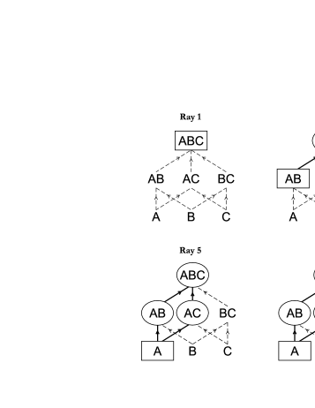
Figure 1: All possible ‘up-sets’ for three parties, up to permutations. Broken arrows indicate which sets have the corresponding element as a subset, i.e broken arrow implies is subset of. Every element that is inside a box or circle is defined as having relative entropy 1. A box indicates that we have chosen the set to have relative entropy 1, where as a circle indicates the set is forced to have relative entropy 1 as one of its subsets also has relative entropy 1. This ‘forcing’ of relative entropy via one of the subsets is represented as a black arrow.

Note that every extremal ray of the relative entropy cone is very well structured and can be defined precisely with up-sets. The standard entropy cone however shows no such structure and its extremal rays, although realised by highly structured states, show far less structure in the actually entropy values of the extremal rays (see Pippenger ; Magnificent:7 ).

IV $\mathbf{\overline{\Lambda_{n}^{*}}=\Lambda_{n}}$

Clearly $\Lambda_{n}^{*}\subset\Lambda_{n}$ since all actual states obey the Lindblad-Uhlmann monotonicity inequalities (5) and (6). Since $\Lambda_{n}$ is closed, we thus get $\overline{\Lambda_{n}^{*}}\subset\Lambda_{n}$.

In this section we will show the opposite inclusion, $\overline{\Lambda_{n}^{*}}\supset\Lambda_{n}$, thus showing equality between the relative entropy cone and the Lindblad-Uhlmann cone.

To show this, it will clearly be enough to show that on every extremal ray of $\Lambda_{n}$ there exists a nonzero vector contained in $\Lambda_{n}^{*}$. In other words, if we can construct a pair of states that has a relative entropy vector on an extremal ray, for all possible extremal rays of $\Lambda_{n}$, then due to approximate dilutability we can find entropy vectors along all points of all extremal rays. Since every point inside a cone can be made with a positive linear combination of points from its extremal rays, we obtain that every point inside the cone can be realised and $\Lambda_{n}=\overline{\Lambda_{n}^{*}}$.

Achieving these states can be identified with classical secret sharing schemes (see for example Stinson ) as we will explain. The formalism for a secret sharing scheme can be defined as follows. Imagine a defined secret bit that we want to share between a number of participants. We want only certain so-called ”authorised” groups of participants to be able to recover the secret exactly, while unauthorised groups of parties get no information about the secret. It is clear that with every authorised group $\cal S$, any group $\cal S^{\prime}\supset\cal S$ will also be authorised. So, the authorised groups will form an up-set called an access structure.

Definition 4

An $n$-party secret sharing scheme for a bit $b$ with access structure $\emptyset\neq\mathbf{U}\subset 2^{[n]},\emptyset\notin\cal\mathbf{U}$, consists of the following

(i)

Random variables $X_{1}(b),X_{2}(b),X_{3}(b),\ldots,X_{n}(b)$, each one associated with a participant labelled $1,\ldots,n$ in the secret sharing scheme. $X_{i}(b)$ takes values in a set ${\cal X}_{i}$.

(ii)

For $\cal S\in\mathbf{U}$, denote $X^{\cal S}(b)=(X_{i}(b)\mathrel{\mathop{\mathchar 58\relax}}i\in\cal S)$, the collection of shares accessible to the group $\cal S$

(iii)

For each $\cal S\in\mathbf{U}$, there is a function $f_{\cal S}\mathrel{\mathop{\mathchar 58\relax}}{\cal X}^{\cal S}\mathrel{\mathop{\mathchar 58\relax}}=\prod_{i\in\cal S}{\cal X}_{i}\rightarrow\{0,1\}$ s.t. $f_{\cal S}(X^{\cal S}(b))=b$. For $\cal S\notin\mathbf{U}$ however, $X^{\cal S}(0)$ and $X^{\cal S}(1)$ have the same distributions.

With this scheme the notion of an up-set is naturally included. Since an authorised group of parties are allowed to recover the secret, adding additional parties must also result in an authorised group since the decoding function can be chosen only to act on the previous authorised group. This is the defining feature of an up-set. To relate this to a quantum information setting, we can construct the following density matrix based on a secret sharing scheme:

$$\rho(b)=\sum_{x_{1}\ldots x_{n}}\Pr\{X_{1}(b)=x_{1},\ldots,X_{n}(b)=x_{n}\}|x_{1}\rangle\!\langle^{|}1\otimes|\langle\rangle|{x_{2}}^{2}\otimes\cdots\otimes|x_{n}\rangle\!\langle^{|}n.$$ (9)

The superscript on the terms of the tensor product denote the label of the share. We denote a partial trace of the matrix as

$$\rho(b)^{\mathcal{S}}=\sum_{x_{j}\mathrel{\mathop{\mathchar 58\relax}}j\in{\cal S}}Pr\{X_{j}(b)=x_{j},\forall j\in{\cal S}\}\bigotimes_{j\in{\cal S}}|x_{j}\rangle\!\langle x_{j}|^{j}.$$ (10)

$\rho(b)^{\cal S}$ has the following properties :

• If ${\cal S}\in{\mathbf{U}}$ then the supporting subspace of $\rho(0)^{\mathcal{S}}$ is orthogonal to that of $\rho(1)^{\mathcal{S}}$ which allows the group ${\cal S}$ to determine the secret bit exactly: $\rho(0)^{\cal S}\perp\rho(1)^{\cal S}$.

• If $\mathcal{S}\neq\mathbf{U}$ then $\rho(0)^{\mathcal{S}}=\rho(1)^{\mathcal{S}}$ and no information about the secret can be achieved.

With this density matrix we can construct the following matrices for use in relative entropy $D(\rho\|\sigma)$:

$$\rho^{\cal S} =\rho(0)^{\cal S},$$ (11)

$$\sigma^{\cal S} =\frac{1}{2}\bigl{(}\rho(0)^{\cal S}+\rho(1)^{\cal S}\bigr{)}.$$ (12)

Note that if $\mathcal{S}\notin\mathbf{U}$ then $\rho^{\cal S}=\sigma^{\cal S}$ and the relative entropy is zero. For ${\cal S}\in\mathbf{U}$, we can calculate the relative entropy as follows:

$$D(\rho^{\cal S}\|\sigma^{\cal S})=\operatorname{Tr}\bigg{[}\rho(0)^{\cal S}\log\rho(0)^{\cal S}-\rho(0)^{\cal S}\log\bigg{(}\frac{\rho(0)^{\cal S}}{2}+\frac{\rho(1)^{\cal S}}{2}\bigg{)}\bigg{]}.$$ (13)

Using $\rho(0)^{\cal S}\perp\rho(1)^{\cal S}$.

$$D(\rho^{\cal S}\|\sigma^{\cal S})=\operatorname{Tr}\bigg{[}\rho(0)^{\cal S}\log\rho(0)^{\cal S}-\rho(0)^{\cal S}\log\frac{\rho(0)^{\cal S}}{2}+\rho(0)^{\cal S}\log\frac{\rho(1)^{\cal S}}{2}\bigg{]}.$$ (14)

Since there are no elements in $\rho(0)^{\cal S}$ that are present in $\rho(1)^{\cal S}$ the third term is zero. Hence expanding the second term

$$D(\rho^{\cal S}\|\sigma^{\cal S}) =\operatorname{Tr}\bigg{[}\rho(0)^{\cal S}\log\rho(0)^{\cal S}-\rho(0)^{\cal S}\log\rho(0)^{\cal S}+\rho(0)^{\cal S}(\log 2)\openone\bigg{]}$$ (15)

$$=(\log 2)\operatorname{Tr}[\rho(0)^{\cal S}]=1.$$ (16)

Note that the relative entropy is constant and independent of the number of elements of ${\cal S}$. Hence we have states from which we can produce relative entropies in the form of up-sets described in Proposition 2 by simply realising a classical secret sharing scheme with the required access structure. There exists a secret sharing scheme for every up-set structure, in fact for every access structure Shamir ; ISN . Therefore for each extremal ray of $\Lambda_{n}$ there is a secret sharing scheme whose density operators according to eqs. (9), (11) and (12) will produce the required relative entropy vector and hence prove that each extremal ray is realisable. Hence we have proved that $\overline{\Lambda_{n}^{*}}=\Lambda_{n}$ and thus that monotonicity under restrictions is the only inequality satisfied by relative entropies.

V Simple secret sharing: threshold schemes

In this section we will describe a simple secret sharing scheme for a specialised access structure known as a threshold scheme. We will then build upon this scheme showing how we can construct schemes for any access structure. The threshold scheme was discovered by Shamir Shamir and allows parties to recover a secret if and only if enough of the parties collaborate, such that their number is beyond a predetermined threshold number of parties. Each party is given a part of the secret which we call a ‘share’ of the secret. There is a total of $n$ shares, one share for each party. A threshold value $k$ is also determined such that if a number of parties get together and pool their shares, if the number of shares they have are greater than or equal to $k$ then they can recover the secret precisely. However, if the number of shares is less than $k$, then no information can be extracted about the secret. Accordingly, these schemed are called $(n,k)$-threshold schemes, depending on the number of parties and the desired threshold value. The construction of the threshold scheme is outlined as follows. The premise for the scheme is based on evaluations of a polynomial. Imagine the following polynomial.

$$y=a_{0}+a_{1}x+a_{2}x^{2}+a_{3}x^{3}+\ldots+a_{m-1}x^{m-1}$$ (17)

We label $a_{0}$ as the secret value and the shares as evaluations of this polynomial at different points. Geometry tells us that we need exactly $m$ evaluations of this polynomial to determine the coefficient $a_{0}$ and that if we have any fewer than $m$ evaluations any value of $a_{0}$ would fit the given points. This means that if we have $m$ or more evaluations we know the secret exactly and if we have fewer than $m$ evaluations we know nothing about the secret. The evaluations of the polynomials becomes the ’shares’ of the scheme and we perform $(n,k)$-threshold scheme the calculations over a finite field. Here is a formulation of the scheme extracted from the original paper by Shamir  Shamir .

• Choose a random $k-1$ degree polynomial $y(x)=a_{0}+a_{1}x+a_{2}x^{2}+\ldots+a_{k-1}x^{k-1}$ and let $s$ be the secret where $s=a_{0}$ i.e. $a_{1},\ldots a_{k-1}$ are chosen independently and uniformly from the field $GF(p)$ of $p$ elements (integer modulo $p$)

• The shares are defined as $D_{1}=y(1),D_{2}=y(2),\ldots,D_{i}=y(i),\ldots,D_{n}=y(n)$.

• Any given subset of $k$ of these $D_{i}$ values together with their indices can find the coefficients of $y(x)$ by interpolation and hence find the value of $s=y(0)$.

• Knowing $k-1$ or fewer shares will not reveal what the value of $s$ as there exists polynomials that will fit the given points in the polynomial and allow $a_{0}=0$ or $a_{0}=1$ with every polynomial equally likely.

• We use a set of integers modulo a prime number $p$ which forms a finite field allowing interpolation.

• Given that the secret is an integer we require $p$ to be larger than both max $s$ and $n$.

• If we only have $k-1$ shares, there is one and only one polynomial that can be constructed for each value of $s$ in $GF(p)$. Since each polynomial is equally likely by construction, no information about the secret can be gained.

This scheme can be easily translated to the quantum density matrix defined in eq. (9). Most of the probabilities in the sum are zero except for the ones that are valid for a polynomial fitting the secret value, with shares labeling that part of the sum. This scheme has a very specific access structure, but we can expand to more general access structures. Consider the number of parties $p$, we can have $n>p$ so that we have more shares than parties, allowing us to distribute multiple shares to single parties. This allows us to have access structures not possible with the simple access structure. Imagine that we require an access structure given in Fig. 2. We require that B and C cannot recover the secret, however if they pool their resources together they can. We also need A to be able to recover the secret independently. Under the normal threshold scheme, we need the threshold to be set at $k=1$ so that single party A can recover the secret. However, this means B and C will independently be also able to recover the secret so we cannot create the required access structure.

However, if we use a scheme with more shares than parties, we can achieve this access structure, see Example 5. Many up-sets can be realised using this modified threshold scheme. The following example provides the required threshold scheme and the resulting density matrices.

Example 5

Imagine an $n=3$ system, each labelled by A,B and C respectively. Consider also the following up-set representing an extremal ray. This is Ray 6 as used in the previous section.

$v_{A}$	$v_{B}$	$v_{C}$	$v_{AB}$	$v_{AC}$	$v_{BC}$	$v_{ABC}$
1	0	0	1	1	1	1

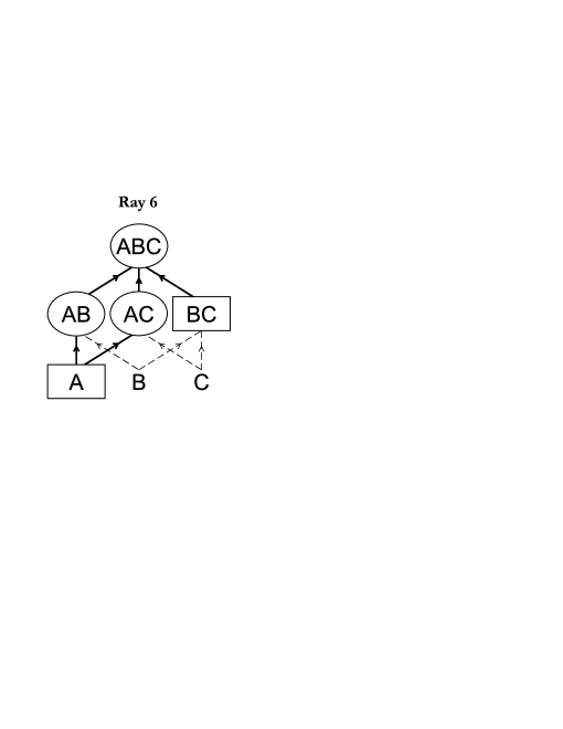
Figure 2: Diagram of up-set used in Example 5

With this up-set we can now construct a secret sharing scheme to represent it. One of the easiest constructions to understand is the threshold scheme. The scheme required is a (4,2) threshold scheme: 4 is the total number of shares, 2 shares or higher required to construct secret. We distribute the shares as follows: two shares to A and only one share to B and one to C. This leads us to the required access structure as shown below.

	$A$	$B$	$C$	$AB$	$AC$	$BC$	$ABC$
Shares	2	1	1	3	3	2	4
Above threshold	$\checkmark$	$\times$	$\times$	$\checkmark$	$\checkmark$	$\checkmark$	$\checkmark$

Since we have a total of four shares, we have to construct the scheme of a finite field of 5. In this example calculations will be assumed to be done over this finite field. Since the threshold is two shares, we only need consider polynomials of order one, since only two or more values are necessary to recover the polynomial of order 1. Therefore the possible polynomials are as follows.

$$y =s$$

$$y =s+x$$

$$y =s+2x$$

$$y =s+3x$$

$$y =s+4x$$

We can now embed this scheme into a quantum system. Each system has the same number of qudits as the corresponding party has shares, with $d$ being large enough to incorporate the finite field values (i.e. in this case d=5). For example system A has two qudits whereas system B only has one. We now construct the density matrices $\rho(0)$ and $\rho(1)$ as follows:

$$\rho(0) =\frac{1}{5}\bigl{(}|0000\rangle\!\langle 0000|+|1234\rangle\!\langle 1234|+|2413\rangle\!\langle 2413|+|3142\rangle\!\langle 3142|+|4321\rangle\!\langle 4321|\bigr{)}$$ (18)

$$\rho(1) =\frac{1}{5}\bigl{(}|1111\rangle\!\langle 1111|+|2340\rangle\!\langle 2340|+|3024\rangle\!\langle 3024|+|4203\rangle\!\langle 4203|+|0432\rangle\!\langle 0432|\bigr{)}$$ (19)

$A$ has the first two qudits, $B$ the third and $C$ the fourth. From this we can construct the overall system described previously. We take $\rho=\rho(0)$ and $\sigma=\frac{\rho(0)+\rho(1)}{2}$ as in eqs. (11) and (12). As examples we may compute

$$\rho_{A} =\frac{1}{5}\bigl{(}|00\rangle\!\langle 00|+|12\rangle\!\langle 12|+|24\rangle\!\langle 24|+|31\rangle\!\langle 31|+|43\rangle\!\langle 43|\bigr{)},$$ (20)

$$\sigma_{A} =\frac{1}{10}\bigl{(}|00\rangle\!\langle 00|+|12\rangle\!\langle 12|+|24\rangle\!\langle 24|+|31\rangle\!\langle 31|+|43\rangle\!\langle 43|\bigr{.}$$

$$\phantom{===}\bigl{.}+|11\rangle\!\langle 11|+|23\rangle\!\langle 23|+|30\rangle\!\langle 30|+|42\rangle\!\langle 42|+|04\rangle\!\langle 04|\bigr{)}.$$ (21)

Therefore it can be verified that the relative entropy of party A is $\log{2}$. Repeating this for party B.

$$\rho_{B}=\frac{1}{5}\bigl{(}|0\rangle\!\langle 0|+|3\rangle\!\langle 3|+|1\rangle\!\langle 1|+|4\rangle\!\langle 4|+|2\rangle\!\langle 2|\bigr{)}=\sigma_{B}.$$ (22)

Therefore the relative entropy for B is 0. All other relative entropies can be verified in this way.

Thus giving unequal number of shares to the parties can achieve more complicated access structures. However not all access structures can be produced in this way. For example imagine that we have a 4 parties A,B,C and D with number of shares in each party being $a,b,c$ and $d$ respectively. We require that A and B can recover the secret and that C and D can recover the secret but no other two party combination. If A and B can recover the secret then their combine total of shares must be greater than $k$ i.e. $a+b\geq k$. Therefore either $a\geq\frac{k}{2}$ or $b\geq\frac{k}{2}$. Similarly we can claim that $c\geq\frac{k}{2}$ or $d\geq\frac{k}{2}$. Say that in this case $a\geq\frac{k}{2},c\geq\frac{k}{2}$. Hence there exists another two party combination, A and C, that have a number of shares greater than $k$ and can recover the secret i.e. $a+c\geq k$. Therefore the access structure is impossible to produce with this scheme. However there are general methods for dealing with arbitrary access structures ISN ; BenLei . These allow us to represent any extremal ray. One strategy is to create a hierarchy of threshold schemes. Here we illustrate the strategy with an example.

Example 6

Imagine an $n=4$ system which we label $A,B,C$ and $D$ respectively. Consider also the following up-set representing an extremal ray.

$v_{A}$	$v_{B}$	$v_{C}$	$v_{D}$	$v_{AB}$	$v_{AC}$	$v_{AD}$	$v_{BC}$	$v_{BD}$	$v_{CD}$	$v_{ABC}$	$v_{ABD}$	$v_{ACD}$	$v_{BCD}$	$v_{ABCD}$
0	0	0	0	1	0	0	0	0	1	1	1	1	1	1

Note that access structure representing this ray requires that no single party has access to the secret and only parties A and B collaborating, and C and D collaborating will be authorised. Also any greater number of parties will always contain an authorised group and are therefore also authorised. The required access structure can be represented by two schemes. This in illustrated in Fig. 3.

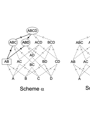
Figure 3: Diagram of up-set used in Example 6

Each scheme requires a $(2,2)$-threshold scheme, 2 total number of shares with a threshold for recovering the secret of 2 shares. We distribute the shares as follows : in one scheme (scheme $\alpha$) we give 1 share to A and 1 share to B. In the other scheme (scheme $\beta$) we give 1 share to C and 1 share to D. This ensures that the secret can be recovered by authorised parties via at least one of the schemes reaching threshold, shown below.

	$A$	$B$	$C$	$D$	$AB$	$AC$	$AD$	$BC$	$BD$	$CD$	$ABC$	$ABD$	$ACD$	$BCD$	$ABCD$
Shares(scheme $\alpha$)	1	1	0	0	2	1	1	1	1	0	2	2	1	1	2
Shares(scheme $\beta$)	0	0	1	1	0	1	1	1	1	2	1	1	2	2	2
Above threshold	$\times$	$\times$	$\times$	$\times$	$\checkmark_{\alpha}$	$\times$	$\times$	$\times$	$\times$	$\checkmark_{\beta}$	$\checkmark_{\alpha}$	$\checkmark_{\alpha}$	$\checkmark_{\beta}$	$\checkmark_{\beta}$	$\checkmark_{\alpha,\beta}$

Since we have a total of two shares for each scheme, we construct the scheme using a finite field of 3 elements. From now on calculations will be assumed to be done over this finite field. Since the threshold is two shares, we only need consider polynomials of order one, since only two or more coordinates are necessary to recover the polynomial of order 1. Therefore the possible polynomials are as follows.

$$y =s$$

$$y =s+x$$

$$y =s+2x$$

In the construction of the quantum density matrix we need to consider all possible set of shares the individual parties can have. The possible combinations are presented in the following tables.

Scheme $\alpha$	Scheme $\beta$	$A$	$B$	$C$	$D$
$y=s$	$y=s$	$0\ast$	$0\ast$	$\ast 0$	$\ast 0$
$y=s$	$y=s+x$	$0\ast$	$0\ast$	$\ast 1$	$\ast 2$
$y=s$	$y=s+2x$	$0\ast$	$0\ast$	$\ast 2$	$\ast 1$
$y=s+x$	$y=s$	$1\ast$	$2\ast$	$\ast 0$	$\ast 0$
$y=s+x$	$y=s+x$	$1\ast$	$2\ast$	$\ast 1$	$\ast 2$
$y=s+x$	$y=s+2x$	$1\ast$	$2\ast$	$\ast 2$	$\ast 1$
$y=s+2x$	$y=s$	$2\ast$	$1\ast$	$\ast 0$	$\ast 0$
$y=s+2x$	$y=s+x$	$2\ast$	$1\ast$	$\ast 1$	$\ast 2$
$y=s+2x$	$y=s+2x$	$2\ast$	$1\ast$	$\ast 2$	$\ast 1$

Table 1: All possible shares for $s=0$

Scheme $\alpha$	Scheme $\beta$	$A$	$B$	$C$	$D$
$y=s$	$y=s$	$1\ast$	$1\ast$	$\ast 1$	$\ast 1$
$y=s$	$y=s+x$	$1\ast$	$1\ast$	$\ast 2$	$\ast 0$
$y=s$	$y=s+2x$	$1\ast$	$1\ast$	$\ast 0$	$\ast 2$
$y=s+x$	$y=s$	$2\ast$	$0\ast$	$\ast 1$	$\ast 1$
$y=s+x$	$y=s+x$	$2\ast$	$0\ast$	$\ast 2$	$\ast 0$
$y=s+x$	$y=s+2x$	$2\ast$	$0\ast$	$\ast 0$	$\ast 2$
$y=s+2x$	$y=s$	$0\ast$	$2\ast$	$\ast 1$	$\ast 1$
$y=s+2x$	$y=s+x$	$0\ast$	$2\ast$	$\ast 2$	$\ast 0$
$y=s+2x$	$y=s+2x$	$0\ast$	$2\ast$	$\ast 0$	$\ast 2$

Table 2: All possible shares for $s=1$

Each party has two registers, one for each scheme. If a party has no share then the register associated with that scheme is put into a fixed state (here $|\ast\rangle_{A},|\ast\rangle_{B},|\ast\rangle_{C},|\ast\rangle_{D}$) which is uncorrelated to the variables for that scheme. Thus the density matrix $\rho(0)$ is

$$\rho(0)=\frac{1}{9} \bigl{(}\ |0{\ast}\rangle\!\langle 0{\ast}|_{A}\,|0{\ast}\rangle\!\langle 0{\ast}|_{B}\,|{\ast}0\rangle\!\langle{\ast}0|_{C}\,|{\ast}0\rangle\!\langle{\ast}0|_{D}+|0{\ast}\rangle\!\langle 0{\ast}|_{A}\,|0{\ast}\rangle\!\langle 0{\ast}|_{B}\,|{\ast}1\rangle\!\langle{\ast}1|_{C}\,|{\ast}2\rangle\!\langle{\ast}2|_{D}$$

$$+|0{\ast}\rangle\!\langle 0{\ast}|_{A}\,|0{\ast}\rangle\!\langle 0{\ast}|_{B}\,|{\ast}2\rangle\!\langle{\ast}2|_{C}\,|{\ast}1\rangle\!\langle{\ast}1|_{D}+|1{\ast}\rangle\!\langle 1{\ast}|_{A}\,|2{\ast}\rangle\!\langle 2{\ast}|_{B}\,|{\ast}0\rangle\!\langle{\ast}0|_{C}\,|{\ast}0\rangle\!\langle{\ast}0|_{D}$$

$$+|1{\ast}\rangle\!\langle 1{\ast}|_{A}\,|2{\ast}\rangle\!\langle 2{\ast}|_{B}\,|{\ast}1\rangle\!\langle{\ast}1|_{C}\,|{\ast}2\rangle\!\langle{\ast}2|_{D}+|1{\ast}\rangle\!\langle 1{\ast}|_{A}\,|2{\ast}\rangle\!\langle 2{\ast}|_{B}\,|{\ast}2\rangle\!\langle{\ast}2|_{C}\,|{\ast}1\rangle\!\langle{\ast}1|_{D}$$

$$+|2{\ast}\rangle\!\langle 2{\ast}|_{A}\,|1{\ast}\rangle\!\langle 1{\ast}|_{B}\,|{\ast}0\rangle\!\langle{\ast}0|_{C}\,|{\ast}0\rangle\!\langle{\ast}0|_{D}+|2{\ast}\rangle\!\langle 2{\ast}|_{A}\,|1{\ast}\rangle\!\langle 1{\ast}|_{B}\,|{\ast}1\rangle\!\langle{\ast}1|_{C}\,|{\ast}2\rangle\!\langle{\ast}2|_{D}$$

$$\phantom{+|0{\ast}\rangle\!\langle 0{\ast}|_{A}\,|2{\ast}\rangle\!\langle 2{\ast}|_{B}\,|{\ast}0\rangle\!\langle{\ast}0|_{C}\,|{\ast}2\rangle\!\langle{\ast}2|_{D}}+|2{\ast}\rangle\!\langle 2{\ast}|_{A}\,|1{\ast}\rangle\!\langle 1{\ast}|_{B}\,|{\ast}2\rangle\!\langle{\ast}2|_{C}\,|{\ast}1\rangle\!\langle{\ast}1|_{D}\bigr{)}.$$

Similarly we can construct $\rho(1)$ by repeating the process but setting the secret bit to be 1, i.e. $|1{\ast}\rangle_{A}|1{\ast}\rangle_{B}|{\ast}1\rangle_{C}|{\ast}1\rangle_{D}$ etc., leading to the density matrix $\rho(1)$:

$$\rho(1)=\frac{1}{9} \bigl{(}\ |1{\ast}\rangle\!\langle 1{\ast}|_{A}\,|1{\ast}\rangle\!\langle 1{\ast}|_{B}\,|{\ast}1\rangle\!\langle{\ast}1|_{C}\,|{\ast}1\rangle\!\langle{\ast}1|_{D}+|1{\ast}\rangle\!\langle 1{\ast}|_{A}\,|1{\ast}\rangle\!\langle 1{\ast}|_{B}\,|{\ast}2\rangle\!\langle{\ast}2|_{C}\,|{\ast}0\rangle\!\langle{\ast}0|_{D}$$

$$+|1{\ast}\rangle\!\langle 1{\ast}|_{A}\,|1{\ast}\rangle\!\langle 1{\ast}|_{B}\,|{\ast}0\rangle\!\langle{\ast}0|_{C}\,|{\ast}2\rangle\!\langle{\ast}2|_{D}+|2{\ast}\rangle\!\langle 2{\ast}|_{A}\,|0{\ast}\rangle\!\langle 0{\ast}|_{B}\,|{\ast}1\rangle\!\langle{\ast}1|_{C}\,|{\ast}1\rangle\!\langle{\ast}1|_{D}$$

$$+|2{\ast}\rangle\!\langle 2{\ast}|_{A}\,|0{\ast}\rangle\!\langle 0{\ast}|_{B}\,|{\ast}2\rangle\!\langle{\ast}2|_{C}\,|{\ast}0\rangle\!\langle{\ast}0|_{D}+|2{\ast}\rangle\!\langle 2{\ast}|_{A}\,|0{\ast}\rangle\!\langle 0{\ast}|_{B}\,|{\ast}0\rangle\!\langle{\ast}0|_{C}\,|{\ast}2\rangle\!\langle{\ast}2|_{D}$$

$$+|0{\ast}\rangle\!\langle 0{\ast}|_{A}\,|2{\ast}\rangle\!\langle 2{\ast}|_{B}\,|{\ast}1\rangle\!\langle{\ast}1|_{C}\,|{\ast}1\rangle\!\langle{\ast}1|_{D}+|0{\ast}\rangle\!\langle 0{\ast}|_{A}\,|2{\ast}\rangle\!\langle 2{\ast}|_{B}\,|{\ast}2\rangle\!\langle{\ast}2|_{C}\,|{\ast}0\rangle\!\langle{\ast}0|_{D}$$

$$\phantom{+|0{\ast}\rangle\!\langle 0{\ast}|_{A}\,|2{\ast}\rangle\!\langle 2{\ast}|_{B}\,|{\ast}0\rangle\!\langle{\ast}0|_{C}\,|{\ast}2\rangle\!\langle{\ast}2|_{D}}+|0{\ast}\rangle\!\langle 0{\ast}|_{A}\,|2{\ast}\rangle\!\langle 2{\ast}|_{B}\,|{\ast}0\rangle\!\langle{\ast}0|_{C}\,|{\ast}2\rangle\!\langle{\ast}2|_{D}\bigr{)}.$$

We notice that in both states $\rho(0)$ and $\rho(1)$ in this example the state $|\ast\rangle_{A}|\ast\rangle_{B}|\ast\rangle_{C}|\ast\rangle_{D}$ factors out so that we could equally well take

$$\rho(0) =\frac{1}{9}\bigl{(}|0000\rangle\!\langle 0000|+|0012\rangle\!\langle 0012|+|0021\rangle\!\langle 0021|+|1200\rangle\!\langle 1200|$$

$$\phantom{==}+|1212\rangle\!\langle 1212|+|1221\rangle\!\langle 1221|+|2100\rangle\!\langle 2100|+|2112\rangle\!\langle 2112|+|2121\rangle\!\langle 2121|\bigr{)},$$ (23)

$$\rho(1) =\frac{1}{9}\bigl{(}|1111\rangle\!\langle 1111|+|1120\rangle\!\langle 1120|+|1102\rangle\!\langle 1102|+|2011\rangle\!\langle 2011|$$

$$\phantom{==}+|2020\rangle\!\langle 2020|+|2002\rangle\!\langle 2002|+|0211\rangle\!\langle 0211|+|0220\rangle\!\langle 0220|+|0202\rangle\!\langle 0202|\bigr{)}.$$ (24)

[Note however that in more complicated examples parties need shares from more than one scheme.] From this we can construct the overall system described previously, and for example for parties $AB$.

$$\rho_{AB} =\frac{1}{3}\bigl{(}|00\rangle\!\langle 00|+|12\rangle\!\langle 12|+|21\rangle\!\langle 21|\bigr{)},$$ (25)

$$\sigma_{AB} =\frac{1}{6}\bigl{(}|00\rangle\!\langle 00|+|12\rangle\!\langle 12|+|21\rangle\!\langle 21|+|11\rangle\!\langle 11|+|20\rangle\!\langle 20|+|02\rangle\!\langle 02|\bigr{)}.$$ (26)

Therefore it can be verified that the relative entropy of parties AB is $\log{2}$. Repeating this for parties BC,

$$\rho_{BC}=\frac{1}{6}\bigl{(}|11\rangle\!\langle 11|+|12\rangle\!\langle 12|+|10\rangle\!\langle 10|+|02\rangle\!\langle 02|+|00\rangle\!\langle 00|+|21\rangle\!\langle 21|+|22\rangle\!\langle 22|+|20\rangle\!\langle 20|\bigr{)}=\sigma_{BC}.$$ (27)

Therefore the relative entropy for BC is 0. All other relative entropies can be verified in this way.

The idea of using a hierarchy of threshold schemes was discovered by Ito, Saito and Nishizeki ISN and requires an exponential number of threshold schemes to represent an access structure. This number of schemes required is irrelevant as long as a scheme exists and we can create the corresponding density matrix. A simpler general access structure was found by Benaloh and Leichter BenLei , which does not use threshold schemes but can be directly translated to the required density matrices in eq. (9).

VI Conclusion

In this paper, we have determined the set of all relative entropy vectors for general states on (general) $n$-party systems: it coincides with the convex cone defined by non-negativity and monotonicity of the relative entropy. We have done this by first showing that the former set in is indeed a convex cone, and then demonstrating that every extremal ray in the latter cone is realised by a specific pair of states. These extremal rays are characterised by up-sets in $2^{[n]}$, and the pairs of states correspond to (classical) secret sharing schemes.

A particular consequence is that the cone of relative entropy vectors is the same for quantum states and for classical probability distributions. This is in marked contrast to the case of entropy vectors, where even for $n=2$ classical and quantum entropy cone differ Pippenger .

Beyond the characterisation in terms of convex geometry, our result also means that, apart from monotonicity, there can be no other univeral relation between the relative entropy values of the reduced states in a composite systems (except that is follows trivially from monotonicty). In this sense, quantum and classical relative entropy is completely characterised by the monotonicity relation.

We are now in a position to go back to our assumption of finite dimensional systems and the demand that all relative entropies are finite. Clearly, if some of the parties are described by infinite dimensional quantum systems, we still have monotonicity Uhlmann , so the relative entropy vectors are all within the Lindblad-Uhlmann cone. In this case, and even in the finite dimensional case some entries in a relative entropy vector may be positive infinity. However, even this does not present a problem, once we realise that the groups where the value is infinite form an up-set, so the vector can indeed be obtained as a limit of finite relative entropy vectors in the Lindblad-Uhlmann cone.

Another mathematical peculiarity is the following: From the proof of achievability of all extremal ray of the Lindblad-Uhlmann cone, we discover that every point in the entropy cone is achievable rather than infinitely approximated, i.e. $\Lambda_{n}=\Lambda_{n}^{*}$. This is due to the fact that every point on all exremal rays can be attained. To see, this, simply choose $\rho(0)$ and $\rho(1)$ in eq. (12) with different weights $p$ and $1-p$ ($0\leq p\leq 1$). Then the calculation following that equation shows that the relative entropy is either $H_{2}(p)$ or $0$ depending on whether ${\cal S}$ is an authorised set or not. By additivity in Lemma 1 we obtain that every point on the extremal rays is realised, hence every point in the Lindblad-Uhlmann cone.

We conclude the paper by commenting briefly on possible connections of our result to the entropy cone, and possibly to the relative entropy of entanglement. In the above arguments we have often used the formula $D(\rho\|\sigma)=-S(\rho)-\operatorname{Tr}\rho\log\sigma$, which means that if we make the restriction $\sigma=\frac{1}{d}\openone$, the maximally mixed state in $d$ dimensions, the relative entropies (now dependent only on $\rho$) evaluate to $\log d-S(\rho)$. Going through the proof of Lemma 1 we see that for any number $n$ of parties, the set of all these relative entropy vectors is also a convex cone, and one might think that its relations would capture all inequalities for the entropy. That this is too optimistic a hope, is indicated by the fact that the relative entropy is expressed by the entropy and a term beyond what can be expressed by general entropies alone (essentially the log of the rank). And it is indeed not the case, since for example the nonegativity of the relative entropy translates into $S(\rho)\leq\log d$. However, the fundamental fact that the entropy $S(\rho)$ is nonnegative, is not captured at all, since that would require an upper bound on the relative entropy depending on the dimension. Still, there may be some less stringent relation between the entropy and the relative entropy cones, whose existence we would like to advertise as an open problem.

- (1) J. Benaloh, J. Leichter, “Generalising Secret Sharing and Monotone Functions.”, Advances in Cryptology, CRYPTO 1998, pp. 27-35, LNCS 403, Springer Verlag, Berlin, 1990.
- (2) C. H. Bennett, D. P. DiVincenzo, J. A. Smolin, W. K. Wootters, “Mixed State entanglement and quantum error correction”, Phys. Rev. A, vol. 54, pp. 3824-3851, 1996.
- (3) N. J. Cerf, C. Adami, “Negative Entropy and Information in quantum mechanics”, Phys. Rev. Lett., vol. 79, pp. 5194-5197, 1997.
- (4) M. Christandl, A. Winter, “Squashed Entanglement – An additive entanglement measure”, J. Math. Phys., vol. 45, no. 3, pp. 829-840, 2004.
- (5) T. M. Cover, J. A. Thomas, Elements of Information Theory, Wiley & Sons, 1991.
- (6) B. Grünbaum, Convex Polytopes, 2nd ed. prepared by V. Kaibel, V. Klee, and G. Ziegler, Graduate Texts in Mathematics 221, Springer Verlag, Berlin, 2003.
- (7) M. Ito, A. Saito, T. Nishizeki “Secret Sharing Schemes releasing General Access Structure”, Proc. IEEE Globecom ’87, pp. 99-102, 1987.
- (8) E. H. Lieb, M. B. Ruskai, “Proof of the Strong Subadditivity of Quantum-Mechanical Entropy”, J. Math. Phys., vol. 14, pp. 1938-1941 , 1973.
- (9) G. Lindblad, “Completey positive maps and entropy inequalities”, Commun. Math. Phys., vol. 40, pp. 147-151, 1975.
- (10) N. Linden, E. Maneva, S. Massar, S. Popescu, D. Roberts, B. Schumacher, J. A. Smolin, A. V. Thapliyal, in preparation (2005).
- (11) N. Linden, A. Winter, “A new inequality for the von Neumann entropy”, Commun. Math. Phys., vol. 259, pp. 129-138, 2005.
- (12) M. A. Nielsen, I. L. Chuang, Quantum Computation and Quantum Information, Cambridge University Press, 2000.
- (13) D. Petz, “Monotonicity of quantum relative entropy revisited”, Rev. Math. Phys., vol. 15, no.1, pp. 79-91, 2003.
- (14) N. Pippenger, “The inequalities of quantum information theory”, IEEE Trans. Inf. Theory, vol. 49, no. 4, pp. 773-789, 2003.
- (15) A. Shamir, “How to Share a Secret”, Commun. ACM, vol. 22, no. 11, pp. 612-613, 1979.
- (16) D. R. Stinson, “An explication of secret sharing schemes”, Designs, Codes and Cryptography, vol. 2, no. 4, pp. 357-390, 1992.
- (17) A. Uhlmann, “Relative Entropy and the Wigner-Yanase-Dyson-Lieb Concavity in an Interpolation Theory”, Commun. Math. Phys., vol. 54, pp. 21-32, 1977.
- (18) V. Vedral, “The Role of Relative Entropy in Quantum Information Theory”, Rev. Mod. Phys., vol. 74, no. 1, pp. 197-234, 2002.
- (19) V. Vedral, M. B. Plenio, “Entanglement measures and purification procedures”, Phys. Rev. A, vol. 57, pp. 1619-1633, 1998.
- (20) V. Vedral, M. B. Plenio, M. A. Rippin, P. L. Knight “Quantifying Entanglement”, Phys. Rev. Lett., vol. 78, pp. 2275-2279, 1996.
- (21) R. W. Yeung, “A Framework for Linear Information Inequalities”, IEEE Trans. Inf. Theory, vol. 43, no. 6, pp. 1924 - 1934, 1997.
- (22) Z. Zhang, R. W. Yeung, “On Characterization of Entropy Function via Information Inequalities”, IEEE Trans. on Inform. Theory, vol. 44, no. 4, pp. 1440-1452, 1998.