UWthPh–2005–23 Maximizing nearest neighbour entanglement in finitely correlated qubit–chains

Abstract

We consider translationally invariant states of an infinite one dimensional chain of qubits or spin-$\frac{1}{2}$ particles. We maximize the entanglement shared by nearest neighbours via a variational approach based on finitely correlated states. We find an upper bound of nearest neighbour concurrence equal to ${\cal C}=0.434095$ which is $0.09\%$ away from the bound ${\cal C}_{\text{W}}=0.434467$ obtained by a completely different procedure. The obtained state maximizing nearest neighbour entanglement seems to approximate the maximally entangled mixed states (MEMS). Further we investigate in detail several other properties of the so obtained optimal state.

I Introduction

The understanding of entanglement in a multipartite quantum system is a central problem of contemporary quantum mechanics, also spreading to statistical and solid state physics. A multipartite quantum system cannot exhibit arbitrary entanglement properties, and the restrictions are far from being straightforward. This fact has several implications on the properties of spin chains and spin lattices, the typical subjects of statistical and solid state physics. This became apparent along with the recent developments of density matrix renormalization group (DMRG) techniques (consult  DMRG for a recent review).

In particular, if one considers a system of two subsystems in a maximally entangled state, neither of the subsystems can, of course, be entangled with anything else. In a system of many quantum bits (qubits, or spin-$\frac{1}{2}$ particles) the limitations on the entanglement of the qubit-pairs are quantified by the Coffman-Kundu-Wootters (CKW) inequalities CKW , for more than three qubits this long standing conjecture was recently proven CKWproof . Finding a quantum state with prescribed pairwise entanglement between each pair is therefore not always possible, and it is a rather involved task Buzek .

In this paper we consider an infinite one dimensional chain of qubits where each qubit is entangled at least with its two nearest neighbours. We impose the constraint of translation invariance: the state should be invariant under all transformations that shift each qubit from its original position $i$ to $i+n$ for some integer $n$. Our main goal is to find the maximal possible achievable entanglement of the nearest neighbours, and study the properties of the so arising chain. This problem is interesting mainly for two reasons. First, because if the bound on nearest neighbour entanglement is optimal, then it serves as a reference point for interpreting entanglement values obtained for real physical systems (such as the antiferromagnetic Heisenberg chain ConnorWooters or lines of ions in a trap which could be used for quantum computations CiracZoller ). Second, because the results contribute to the knowledge on the possible structures of distributed entanglement in systems of (infinitely) many subsystems.

This question was also addressed by Wootters WoottersEntangledChains . Via a certain procedure he succeeded in constructing such translation invariant entangled chains in which the maximal achievable concurrence is ${\cal C}_{\text{W}}=0.434467$ which corresponds to a value of entanglement of formation of $E_{f}=0.284934$ ebits. This value is below ${\cal C}_{\text{CKW}}=1/\sqrt{2}$, the limit that the CKW inequalities would allow for, in the case when each quantum bit is maximally entangled with the rest of the system, while the bipartite entanglement is restricted to the nearest neighbours. The concurrence ${\cal C}_{W}$ is conjectured to be an absolute bound, but this fact is not proven. A challenging question in this context is if one can go beyond ${\cal C}_{W}$, or even reach ${\cal C}_{\text{CKW}}$.

In this paper we attack the problem in a different way, related to the DMRG method. This latter is found to be a variational method in terms of the so-called matrix product states (MPS) FNW , equivalent to a sequence of entanglement swappings DMRGinf . The MPSs constitute a representation of the pure state of a finite number of qubits. For each qubit of the system an auxiliary finite dimensional Hilbert space is considered. The state is described by projectors acting between the auxiliary space and the space of the system under consideration. They are very suitable for approximating ground states of Hamiltonians in a numerically efficient way where the approximation lies on the dimensionality of the auxiliary system. The infinite chain can be studied as a limit, assuming periodic boundary conditions. This attitude is equivalent to a different formulation, termed finitely correlated states (FCS). A pure state of the whole translationally invariant chain is encoded into a state of an auxiliary system and a completely positive (CP) map. In this framework, the density operator for any finite subset of the system can be constructed by the successive application of the CP map, while the auxiliary system models the rest of the system from the point of view of quantum correlations. All translational invariant states can be approximated in that way with an accuracy which may depend on the dimension of the auxiliary system.

The entanglement distribution of such chains has been already studied in Refs. BHN1 ; BHN2 under the restriction of $2$ dimensional auxiliary systems endnote1 .

We shall use a specific subset of such FCS as an ansatz to maximize nearest neighbour entanglement in a translationally invariant infinite chain of qubits. This approach has several advantages. First, it provides us explicitly with a well-defined pure state on the whole chain. Second, we can study a class of quantum states different to the one studied in Ref. WoottersEntangledChains . Third, we can also investigate higher correlations as next nearest neighbour entanglement and entanglement of one qubit with the rest of the chain.

Thus we can study the entanglement distributed along the chain, however, we focus mainly on maximizing nearest neighbour entanglement and the properties of such an optimal state regarding the entanglement of next nearest, and further neighbours. For two dimensional auxiliary systems we have analytical results describing the properties of entanglement of such an entangled chain and for higher dimensions we have performed a numerical optimization. We have found that the achievable nearest neighbours entanglement seems to converge fast to Wootters’ bound ${\cal C}_{\text{W}}$.

This paper is organized as follows. Section II is devoted to the construction of the states of translationally invariant finitely correlated chains utilized in this paper. In Section III analytical results are presented for the maximization of the nearest neighbour entanglement for the case of low dimensional auxiliary Hilbert spaces, to give an insight into the nature of the problem. In Section IV our numerical results are presented for higher dimensionalities, while in Section V the properties of the so found optimal states are discussed. In Section VI our results are summarized, and conclusions are drawn.

II Construction of the translation invariant entangled chain

We consider an infinite ensemble of qubits arranged along a line. The first question we address is what we mean by the word “state” as applied to infinitely many qubits. We adopt the standard approach described in e.g. Ref. bookBrotteliRobinson . A state $\omega$ of the infinite chain is a functional that assigns to every finite set of local operators $A_{[1,n]}=A_{1}\otimes A_{2}\dots\otimes A_{n}$ a normalized density matrix $\omega(A_{[1,n]})$ describing the properties of the of $n$ qubits. Moreover one demands that if one considers a subset of local operators $A_{[1,k]}$ of the set $A_{[1,n]}$ then the state $\omega(A_{[1,k]})$ has to be obtained by taking the partial trace of $\omega(A_{[1,n]})$ over the qubits not in $A_{[1,n]}$.

Before describing the rather mathematical construction in detail, we outline first the idea behind it. The trick is to describe the part of the chain in which one is not interested in by a density matrix on an auxiliary Hilbert space ${\cal H}_{B}$, a local operator of the bounded operators $\cal{B}({\cal H}_{B})$ and a completely positive map which maps tensor products of such an auxiliary local operator and the local operator of one qubit $A_{i}$ always back into $\cal{B}({\cal H}_{B})$. In this way the completely positive map ensures that one only archives permitted states of a qubit or more qubits in such an infinite chain. It is clear that the set of the permitted and thus realized states of a qubit or more qubits of the chain can increase if the dimension of the auxiliary system describing the “rest of the chain” is increased. Further one has to carefully choose the appropriate completely positive maps in order to study the class of permitted one or more qubit states one is interested in.

Explicit examples for choices of the completely positive map for increasing dimensions of the auxiliary system which maximize nearest neighbour entanglement (our main goal) are then given in Sec. III, but let us first proceed with the construction of the finitely correlated states in more detail.

II.1 Construction of finitely correlated states (FCS)

In the following we summarize the exact mathematical construction of translationally invariant finitely correlated states according to Ref. FNW . We denote by $\mathcal{A}_{\mathbb{Z}}$ an infinite spin-chain, the spins at sites $i\in\mathbb{Z}$ being described by the algebra $({\cal A})_{i}={\bf M}_{2}$ of $2\times 2$ complex matrices, i.e. we describe spin-$\frac{1}{2}$ particles or generally qubits. The infinite algebra $\mathcal{A}_{\mathbb{Z}}$ arises as a suitable limit of the local tensor-product algebras ${\cal A}_{[-n,n]}:=\otimes_{j=-n}^{n}(\mathcal{A})_{j}$. Any state $\omega$ over $\mathcal{A}_{\mathbb{Z}}$ is specified by density matrices $\rho_{[1,n]}$ defining the action of $\omega$ as an expectation over local operators $A_{[1,n]}\in\mathcal{A}_{[1,n]}$:

$$\omega(A_{[1,n]}) = {\rm Tr}_{[1,n]}\Bigl{(}\rho_{[1,n]}\,A_{1}\otimes A_{2}\otimes\dots A_{n}\Bigr{)}$$ (1)

$$= {\rm Tr}_{[1,n]}\Bigl{(}\rho_{[1,n]}\,A_{[1,n]}\Bigr{)}\ .$$

The $\rho_{[1,n]}$’s must satisfy the compatibility conditions, i.e. acting locally on the $n+1$ qubit with a unity operator should give the same expectation value

$$\omega(A_{[1,n]}) = \hbox{Tr}_{n+1}\Bigl{(}\rho_{[1,n+1]}\,A_{[1,n]}\otimes\mathbbm{1}_{n+1}\Bigl{)}$$ (2)

$$= \hbox{Tr}_{[1,n]}\Bigl{(}\rho_{[1,n]}\,A_{[1,n]}\Bigr{)}\ .$$

Whereas, translation-invariance requires that doing no operation on the first qubit should also do no change to the expectation value, i.e. shifting the line of qubits by one (generally by an integer)

$$\omega(A_{[1,n]}) = \hbox{Tr}_{n+1}\Bigl{(}\rho_{[1,n+1]}\,\mathbbm{1}_{1}\otimes A_{[2,n+1]}\Bigl{)}$$ (3)

$$= \hbox{Tr}_{[1,n]}\Bigl{(}\rho_{[1,n]}\,A_{[1,n]}\Bigr{)}\ .$$

The class of translation-invariant finitely correlated states (FCS) over $\mathcal{A}_{\mathbb{Z}}$ is defined by a triple $(\mathcal{B},\rho,\mathbb{E})$ where $\mathcal{B}$ is a $b\times b$ matrix algebra $\mathcal{B}$, $\rho_{B}\in\mathcal{B}$ a density matrix and $\mathbb{E}:\mathcal{A}\otimes\mathcal{B}\mapsto\mathcal{B}$ a completely positive unital map, which in Kraus form reads

$$\mathbb{E}(A\otimes B)=\sum_{j}V_{j}(A\otimes B)V_{j}^{\dagger}\ ,\quad V_{j}:\mathbb{C}^{2}\otimes\mathbb{C}^{b}\mapsto\mathbb{C}^{b}\ ,$$ (4)

with $A\in\mathcal{A}$ and $B\in\mathcal{B}$. Unitality means that identities are preserved

$$\mathbb{E}(\mathbbm{1}_{\mathcal{A}}\otimes\mathbbm{1}_{\mathcal{B}})=\mathbbm{1}_{\mathcal{B}}\quad\textit{ unitality}\,.$$ (5)

Let $\mathbb{E}^{(1)}(A):=\mathbb{E}(A\otimes\mathbbm{1}_{\mathcal{B}})$; this defines a completely positive map from $\mathcal{A}$ into $\mathcal{B}$. Analogously, the recursive compositions $\mathbb{E}^{(n)}:=\mathbb{E}\circ\Bigl{(}{\rm id}_{\mathcal{A}}\otimes\mathbb{E}^{(n-1)}\Bigr{)}$ are completely positive maps from $\mathcal{A}_{[1,n]}$ into $\mathcal{B}$. Setting

$$\omega(A_{[1,n]})=\hbox{Tr}\Bigl{(}\rho_{[1,n]}\,A_{[1,n]}\Bigr{)} := {\rm Tr}_{{\cal B}}\big{(}\rho_{B}\,\underbrace{\mathbb{E}\big{[}A_{1}\otimes\underbrace{\mathbb{E}\big{[}A_{2}\otimes\underbrace{\mathbb{E}\big{[}\dots\otimes\big{[}\underbrace{A_{n}\otimes\mathbbm{1}_{{\cal B}}}_{\in{\cal B}}\big{]}\dots\big{]}}_{\in{\cal B}}\big{]}}_{\in{\cal B}}\big{]}}_{\in{\cal B}}\big{)}$$ (6)

$$= {\rm Tr}_{{\cal{B}}}\Bigl{(}\rho_{B}\,\mathbb{E}^{(n)}\Bigl{(}A_{[1,n]}\Bigr{)}\Bigr{)}\ ,$$

the r.h.s. recursively defines local density matrices $\rho_{[1,n]}$ over $\mathcal{A}_{[1,n]}$ and a total state $\omega$ on $\mathcal{A}_{\mathbb{Z}}$. Translation invariance condition Eq. (3) can be formulated as

$${\rm Tr}_{\mathcal{B}}\left(\rho_{B}\,\mathbb{E}\left(\mathbbm{1}_{\mathcal{A}}\otimes B\right)\right)={\rm Tr}_{\mathcal{B}}(\rho_{B}\,B)\quad\forall\,B\in\mathcal{B}\,.$$ (7)

II.2 Constraints of unitality and translational invariance

Concretely, we choose $\mathcal{B}={\bf M}_{b}$ ($b\times b$ complex matrices) and $\mathbb{E}$ like in (4) but with just one Kraus operator $V:\mathbb{C}^{2}\otimes\mathbb{C}^{b}\mapsto\mathbb{C}^{b}$. (Note that this restriction does not decrease the generality, as the introduction of further Kraus operators can be avoided by increasing the dimensionality $b$.) This is such that $V|a_{i}\otimes\psi\rangle=v_{i}|\psi\rangle$, $V^{\dagger}|\psi\rangle=\sum_{i=1}^{2}|a_{i}\rangle\otimes v_{i}^{\dagger}|\psi\rangle$ and with the one qubit operator $A=\sum a_{ij}\ |a_{i}\rangle\langle a_{j}|$

$$\mathbb{E}\Bigl{(}|a_{i}\rangle\langle a_{j}|\otimes B\Bigr{)}=v_{i}\,B\,v_{j}^{\dagger}\ ,\quad B\in\mathcal{B}\ ,$$ (8)

where $|a_{1,2}\rangle\in\mathbb{C}^{2}$ are orthonormal and $v_{1,2}$ $b\times b$ matrices. In this notation the unitality and translation invariance reads for the two matrices

$$v_{1}v_{1}^{\dagger}+v_{2}v_{2}^{\dagger}=\mathbbm{1}_{\mathcal{B}}\quad unitality$$ (9)

$$\sum_{i=1}^{2}v_{i}^{\dagger}\ \rho_{B}\ v_{i}=\rho_{B}\quad\text{{translation invariance}}\,.$$ (10)

If there exists a unique $\rho$ fulfilling the previous condition, the resulting translation–invariant FCS are pure states over $\mathcal{A}_{\mathbb{Z}}$ FNW , namely they cannot be decomposed as mixtures of other states. These pure states can be interpreted as ground states for appropriately constructed Hamiltonians of finite range FNW . It is also shown that this class of states is dense in the set of all translation invariant states FNW2 .

The two conditions Eq. (9), Eq. (10) can as well be interpreted in the context of open quantum systems. I.e. $\rho_{B}$ is the state of some open quantum system where the $v$’s are the operation elements for the quantum operation. These operation elements satisfy the well known completeness relation (first condition) which leads to trace conservation of the completely positive map, i.e. no information of the whole system ($B$ plus environment) is lost. The second equation (condition 2) can then be interpreted as searching for states which are invariant under these interactions.

II.3 Density matrices for a subset of qubits in the chain

Let us first consider the state of one qubit in the chain, defined in Eq.(6)

$$\omega(A) = {\rm Tr}_{A}\big{(}\rho_{[1]}\ A\otimes\mathbbm{1}_{B}\big{)}:={\rm Tr}_{B}\big{(}\rho_{B}\ \mathbb{E}(A\otimes\mathbbm{1}_{B})\big{)}$$

$$= {\rm Tr}_{B}\left(\rho_{B}\ \mathbb{E}\left(\sum a_{ij}\ |a_{i}\rangle\langle a_{j}|\otimes\mathbbm{1}_{B}\right)\right)$$

$$= {\rm Tr}_{B}\big{(}\rho_{B}\sum a_{ij}\ v_{i}\mathbbm{1}_{B}v_{j}^{\dagger}\big{)}$$

$$= {\rm Tr}_{B}\left(\sum a_{ij}\ v_{j}^{\dagger}\rho_{B}v_{i}\ \mathbbm{1}_{B}\right)$$

$$= {\rm Tr}_{A\otimes B}\left(\sum a_{ij}\ {\rm Tr}_{B}\left(v_{j}^{\dagger}\rho_{B}v_{i}\right)\ |a_{i}\rangle\langle a_{j}|\otimes\mathbbm{1}_{B}\right)$$

where we have used the cyclic property of the trace – ${\rm Tr}(XY)={\rm Tr}(YX)$ – and the fact that the trace operation is invariant under the map $\mathbb{F}:{\cal B}\rightarrow{\cal A}\otimes{\cal B}$ dual to $\mathbb{E}:{\cal A}\otimes{\cal B}\rightarrow{\cal B}$. This is defined by

$$\mathbb{F}(B):=\sum_{i,j=2}^{2}|a_{j}\rangle\langle a_{i}|\otimes v_{i}^{\dagger}Bv_{j}\;.$$ (12)

Hence comparing the last term with the first one we find that the density matrix of a qubit in the chain is given by

$$\rho_{[1]} = \rho_{1}=\sum_{i,j}^{2}|a_{j}\rangle\langle a_{i}|\ {\rm Tr}\big{(}v_{j}^{\dagger}\,\rho_{B}\,v_{i}\big{)}$$ (15)

$$= \left(\begin{array}[]{cc}{\rm Tr}\big{(}v_{1}^{\dagger}\,\rho_{B}\,v_{1}\big{)}&{\rm Tr}\big{(}v_{1}^{\dagger}\,\rho_{B}\,v_{2}\big{)}\\ {\rm Tr}\big{(}v_{2}^{\dagger}\,\rho_{B}\,v_{1}\big{)}&{\rm Tr}\big{(}v_{2}^{\dagger}\,\rho_{B}\,v_{2}\big{)}\end{array}\right)\;.$$

Now let us investigate the nearest neighbour state, i.e. Eq.(6) by setting $n=2$, thus we have $A_{[1,2]}=A_{1}\otimes A_{2}$ and

$$\hbox{Tr}\Bigl{(}\rho_{[1,2]}\,A_{1}\otimes A_{2}\Bigr{)}:={\rm Tr}_{B}\Bigl{(}\rho_{B}\,\mathbb{E}\Bigl{(}A_{1}\otimes\mathbb{E}\Bigl{(}A_{2}\otimes\mathbbm{1}_{B}\Bigr{)}\Bigr{)}\ .$$ (16)

Again using the properties of the trace-operation, the action of $\mathbb{E}$ becomes the action of its dual map $\mathbb{F}$

$$\hbox{Tr}\Bigl{(}\rho_{[1,2]}\,A_{1}\otimes A_{2}\Bigr{)}:={\rm Tr}_{A\otimes B}\Bigl{(}\mathbb{F}(\rho_{B})\,A_{1}\otimes\mathbb{E}\Bigl{(}A_{2}\otimes\mathbbm{1}_{B}\Bigr{)}\Bigr{)}\ .$$ (17)

This provides a state $\rho_{\mathcal{A}\otimes\mathcal{B}}:=\mathbb{F}(\rho_{B})=V^{\dagger}\,\rho_{B}\,V$ on $\mathcal{A}\otimes\mathcal{B}$:

$$\rho_{\mathcal{A}\otimes\mathcal{B}}=\sum_{s,t=1}^{2}|s\rangle\langle t|\,\otimes\,v^{\dagger}_{s}\,\rho_{B}\,v_{t}=\begin{pmatrix}v_{1}^{\dagger}\,\rho_{B}\,v_{1}&v_{1}^{\dagger}\,\rho_{B}\,v_{2}\cr v_{2}^{\dagger}\,\rho_{B}\,v_{1}&v_{2}^{\dagger}\,\rho_{B}\,v_{2}\end{pmatrix}$$ (18)

which encodes the properties of all the correlations between one site with the rest of the whole chain.

The right hand side of Eq.(17) reads $\hbox{Tr}_{\mathcal{A}\otimes\mathcal{B}}\Bigl{(}\rho_{\mathcal{A}\otimes\mathcal{B}}\,A_{1}\otimes\mathbb{E}\left(A_{2}\otimes\mathbbm{1}_{\mathcal{B}}\right)\Bigr{)}$, by turning ${\rm id}_{\mathcal{A}}\otimes\mathbb{E}$ into its dual, nearest-neighbours states arise as $\rho_{12}:=\rho_{[1,2]}=\hbox{Tr}_{\mathcal{B}}\Bigl{(}{\rm id}_{\mathcal{A}}\otimes\mathbb{F}(\rho_{\mathcal{A}\otimes\mathcal{B}})\Bigr{)}$ which reads

$$\rho_{12} = \sum_{ij=1}^{2}|i\rangle\langle j|\otimes\begin{pmatrix}R_{1ij1}&R_{1ij2}\cr R_{2ij1}&R_{2ij2}\end{pmatrix}\ ,$$ (19)

where $R_{ijlm}={\rm Tr}(v_{i}^{\dagger}v_{j}^{\dagger}\;\rho_{B}\;v_{l}v_{m})$.

In general local density matrices are constructed by

$$\rho_{[1,n]}\;=\;\sum_{{\bf s},{\bf t}}|{{\bf s}}\rangle\langle{\bf t}|\;{\rm Tr}(v_{{\bf s}}^{\dagger}\,\rho_{B}\,v_{{\bf t}})\ ,$$ (20)

where $|{{\bf s}}\rangle=|s_{1}\otimes s_{2}\otimes\cdots s_{n}\rangle$, $v_{\bf t}:=v_{t_{1}}\cdots v_{t_{n}}$.

III Maximizing nearest neighbour entanglement

III.1 General discussion for an optimal choice of $v_{1}$

Our main goal is to maximize the nearest neighbour entanglement of state Eq. (19)

$$\rho_{12} = \begin{pmatrix}{\rm Tr}(v_{1}^{\dagger}v_{1}^{\dagger}\;\rho_{B}\;v_{1}v_{1})&{\rm Tr}(v_{1}^{\dagger}v_{1}^{\dagger}\;\rho_{B}\;v_{1}v_{2})&{\rm Tr}(v_{1}^{\dagger}v_{1}^{\dagger}\;\rho_{B}\;v_{2}v_{1})&{\rm Tr}(v_{1}^{\dagger}v_{1}^{\dagger}\;\rho_{B}\;v_{2}v_{2})\cr{\rm Tr}(v_{2}^{\dagger}v_{1}^{\dagger}\;\rho_{B}\;v_{1}v_{1})&{\rm Tr}(v_{2}^{\dagger}v_{1}^{\dagger}\;\rho_{B}\;v_{1}v_{2})&{\rm Tr}(v_{2}^{\dagger}v_{1}^{\dagger}\;\rho_{B}\;v_{2}v_{1})&{\rm Tr}(v_{2}^{\dagger}v_{1}^{\dagger}\;\rho_{B}\;v_{2}v_{2})\cr{\rm Tr}(v_{1}^{\dagger}v_{2}^{\dagger}\;\rho_{B}\;v_{1}v_{1})&{\rm Tr}(v_{1}^{\dagger}v_{2}^{\dagger}\;\rho_{B}\;v_{1}v_{2})&{\rm Tr}(v_{1}^{\dagger}v_{2}^{\dagger}\;\rho_{B}\;v_{2}v_{1})&{\rm Tr}(v_{1}^{\dagger}v_{2}^{\dagger}\;\rho_{B}\;v_{2}v_{2})\cr{\rm Tr}(v_{2}^{\dagger}v_{2}^{\dagger}\;\rho_{B}\;v_{1}v_{1})&{\rm Tr}(v_{2}^{\dagger}v_{2}^{\dagger}\;\rho_{B}\;v_{1}v_{2})&{\rm Tr}(v_{2}^{\dagger}v_{2}^{\dagger}\;\rho_{B}\;v_{2}v_{1})&{\rm Tr}(v_{2}^{\dagger}v_{2}^{\dagger}\;\rho_{B}\;v_{2}v_{2})\cr\end{pmatrix}\ .$$ (21)

To do so we have to choose appropriate matrices $v_{1},v_{2}$ satisfying the condition in Eq. (9) and then to derive a unique $\rho_{B}$ satisfying the condition in Eq. (10). This then defines the nearest neighbour entanglement given by the density matrix above.

What are appropriate choices for $v_{1}$?

Obviously the entanglement shared by two neighbouring qubits in a chain cannot be maximal, e.g. one of the four pure entangled Bell type states ($|\phi^{\pm}\rangle=\frac{1}{\sqrt{2}}\{|00\rangle\pm|11\rangle\},|\psi^{\pm}\rangle=\frac{1}{\sqrt{2}}\{|01\rangle\pm|01\rangle\}$). In this case every other qubit has to be disentangled with that pair. Therefore the reduced state of the infinite chain we are looking for is not pure. On the other hand it should be far away from the tracial state (i.e. the complete mixture) as well. It seems to be plausible though not conclusive that the reduced state vanishes on some subspace. Considering the basis states $|00\rangle,|11\rangle,|01\rangle,|10\rangle$ we notice that if we choose $|01\rangle$ states then because of translation invariance we need as well $|10\rangle$ states. Thus we expect our reduced state to be orthogonal to a separable pure state, e.g. $|00\rangle$.

Translated to our nearest neighbour state Eq.(21) we need that e.g. ${\rm Tr}(v_{1}^{\dagger}v_{1}^{\dagger}\,\rho_{B}\,v_{1}v_{1})$ vanishes. Since $\rho_{B}$ has to be strictly positive (otherwise we could reduce the dimension of ${\cal B}$) it follows that $v_{1}$ has to be nilpotent, i.e. $v_{1}v_{1}=\mathbf{0}$. Then the nearest neighbour density matrix Eq.(21) gets the form

$$\rho_{12} = \begin{pmatrix}0&0&0&0\cr 0&{\rm Tr}(v_{2}^{\dagger}v_{1}^{\dagger}\;\rho_{B}\;v_{1}v_{2})&{\rm Tr}(v_{2}^{\dagger}v_{1}^{\dagger}\;\rho_{B}\;v_{2}v_{1})&{\rm Tr}(v_{2}^{\dagger}v_{1}^{\dagger}\;\rho_{B}\;v_{2}v_{2})\cr 0&{\rm Tr}(v_{1}^{\dagger}v_{2}^{\dagger}\;\rho_{B}\;v_{1}v_{2})&{\rm Tr}(v_{1}^{\dagger}v_{2}^{\dagger}\;\rho_{B}\;v_{2}v_{1})&{\rm Tr}(v_{1}^{\dagger}v_{2}^{\dagger}\;\rho_{B}\;v_{2}v_{2})\cr 0&{\rm Tr}(v_{2}^{\dagger}v_{2}^{\dagger}\;\rho_{B}\;v_{1}v_{2})&{\rm Tr}(v_{2}^{\dagger}v_{2}^{\dagger}\;\rho_{B}\;v_{2}v_{1})&{\rm Tr}(v_{2}^{\dagger}v_{2}^{\dagger}\;\rho_{B}\;v_{2}v_{2})\cr\end{pmatrix}$$ (26)

$$= \begin{pmatrix}0&0&0&0\cr 0&{\rm Tr}(v_{1}^{\dagger}\;\rho_{B}\;v_{1})&{\rm Tr}(v_{2}^{\dagger}v_{1}^{\dagger}\;\rho_{B}\;v_{2}v_{1})&{\rm Tr}(v_{1}^{\dagger}\;\rho_{B}\;v_{2})\cr 0&{\rm Tr}(v_{1}^{\dagger}v_{2}^{\dagger}\;\rho_{B}\;v_{1}v_{2})&{\rm Tr}(v_{1}^{\dagger}\;\rho_{B}\;v_{1})&{\rm Tr}(v_{1}^{\dagger}\;\rho_{B}\;v_{2})\cr 0&{\rm Tr}(v_{2}^{\dagger}\;\rho_{B}\;v_{1})&{\rm Tr}(v_{2}^{\dagger}\;\rho_{B}\;v_{1})&1-2\,{\rm Tr}(v_{1}^{\dagger}\;\rho_{B}\;v_{1})\cr\end{pmatrix}$$

$$= \left(\begin{array}[]{cccc}0&0&0&0\\ 0&A&B&C\\ 0&B^{*}&A&C\\ 0&C^{*}&C^{*}&1-2A\end{array}\right)$$

This form of the density matrix is similar to the choice in Ref. WoottersEntangledChains except that $C$ is required to be equal zero there. It means that the state considered in the reference is also invariant under local rotation of one qubit around the $x$– and $y$–axis, a crucial assumption in the construction. As we drop this assumption, we can test another class of candidates within our framework.

Let us now discuss the properties of a density matrix of the form Eq. (III.1). Its eigenvalues are $\{0,A-|B|,1-(A-|B|)\pm\sqrt{(3A+|B|-1)^{2}+8|C|^{2}}\}$ and $A\in[0,1/2]$. First we consider its purity as measured by ${\rm Tr}\rho_{12}^{2}$ which equals to $1-4A+6A^{2}+2|B|^{2}+4|C|^{2}$ and the purity for the reduced matrix, i.e. the one–qubit state, equals to $Tr\rho_{1}^{2}=1-2A+2A^{2}+2|C|^{2}$. Intuitively, we expect the entanglement to increase for a density matrix becoming purer, while the purity of the one–qubit state should decrease. However we will notice that for the two–qubit state the opposite is true.

As a measure of entanglement we use the concurrence ${\cal C}$, introduced by Hill and Wootters WoottersHillConcurrence ; WoottersConcurrence , which is a monotonically increasing function of the entanglement of formation Benn . The concurrence of a density matrix $\rho$ is given by $\mathcal{C}(\rho)=\max\{0,\lambda_{1}-\lambda_{2}-\lambda_{3}-\lambda_{4}\}$, where $\lambda_{j}$ are the square roots of the eigenvalues in decreasing order of the matrix $\rho\widetilde{\rho}$ where $\widetilde{\rho}=(\sigma_{y}\otimes\sigma_{y})\rho^{*}(\sigma_{y}\otimes\sigma_{y})$ and $\rho^{*}$ denotes complex conjugation in the standard basis. For the above form of density matrices the eigenvalues $\sqrt{\rho\tilde{\rho}}=\{A+|B|,A-|B|,0,0\}$ are independent of $C$ and the concurrence is simply ${\cal C}(\rho_{12})=2\,|B|$. Clearly, we have separability only for vanishing $|B|$.

Another useful quantity is concurrence of assistance Entass ; Cass which is defined as the sum of the square roots of the eigenvalues of $\rho\widetilde{\rho}$, i.e. in our case its simply given by ${\cal C}_{\text{ass}}(\rho_{12})=2A$. This quantity characterizes the maximum entanglement of a selected pair of qubits available on average when the rest of the system is subjected to measurements.

In order to maximize nearest neighbour entanglement we have to maximize the function

$${\cal C}(\rho_{12})=2\,\left|B\right|=2\,\left|{\rm Tr}(v_{2}^{\dagger}v_{1}^{\dagger}\;\rho_{B}\;v_{2}v_{1})\right|\,.$$ (27)

There is an additional symmetry of the nearest neighbour state, namely $\rho_{12}\rightarrow\rho_{12}^{*}$ does not change the amount of entanglement. For dimension $b=2$ the only effect is to introduce irrelevant phase factors to ${\rm Tr}(v_{2}^{\dagger}v_{1}^{\dagger}\;\rho_{B}\;v_{2}v_{1})$. Though for higher dimensions $b$ this is not the case, we restrict ourselves to real generators as a natural choice to reduce the set of parameters in the calculations. We have checked complex extensions numerically in the region of the obtained maxima where we always have found that it only reduces the amount of entanglement.

In the next section we analyze the case of auxiliary matrices of dimension $2$ where we can give analytical solutions and analyze the generalization for higher dimension.

III.2 Analytical results

For dimension $b=2$ we can give analytical results and go through the whole calculation in order to understand the procedure in more detail and its generalization for higher dimensions. This will also strengthen our assumption for the generators of the completely unital map $\mathcal{E}$. First we investigate the set of solutions $\rho_{B}$ for a nilpotent $v_{1}$ and its generalization for higher dimensions. Then we discuss the implementation to the entanglement to the nearest and next-nearest neighbours.

III.2.1 Solutions for the auxiliary density matrix $\rho_{B}$

We have to solve the two conditions: unitality Eq. (9) and translation invariance Eq. (10). In $b=2$ dimensions the only nilpotent matrices are the ladder operators where we choose without loss of generality one of them with a weight $\cos\alpha_{1}$:

$$v_{1} = \cos{\alpha_{1}}\left(\begin{array}[]{cc}0&0\\ 1&0\end{array}\right)\,,$$ (30)

$$v_{2} = \left(\begin{array}[]{cc}1&0\\ 0&\sin{\alpha_{1}}\end{array}\right).\left(\begin{array}[]{cc}\cos{\phi_{1}}&\sin{\phi_{1}}\\ -\sin{\phi_{1}}&\cos{\phi_{1}}\end{array}\right)\,,$$ (35)

where $v_{2}$ is the most general (real) solution satisfying the unitality condition in Eq. Eq. (9).

Let us now discuss the solutions for the auxiliary $\rho_{B}$, conditions in Eq. (10). The set of possible density matrices which are invariant under the above chosen interaction is illustrated in Fig. 1, where we used the Bloch sphere representation. Every one–qubit state can be decomposed into three Pauli matrices

$$\rho_{B} = \frac{1}{2}(\mathbbm{1}_{2}+n_{i}^{(\text{Bloch})}\sigma^{i}),\qquad n_{i}^{(\text{Bloch})}\in\mathbbm{R}\,,$$ (36)

$$\;\sum_{i}(n_{i}^{(\text{Bloch})})^{2}=\left|\vec{n}^{\,(Bloch)}\right|^{2}\leq 1\,.$$

For $\left|\vec{n}_{(Bloch)}\right|^{2}<1$ the state is mixed (corresponding to Tr$\,\rho^{2}<1$) whereas for $\left|\vec{n}^{\,(Bloch)}\right|^{2}=1$ the state is pure (Tr$\,\rho^{2}=1$). This real three dimensional vector $\vec{n}^{(\text{Bloch})}$ is called the Bloch vector and thus the state space of a qubit can be represented by a sphere, where the vectors with $|\vec{n}^{\,(Bloch)}|=1$ are pure and cover the surface of the sphere, inside the sphere we have all mixed states and the origin represents the totally mixed state, i.e. the tracial state. As we consider real generators of the interaction the $y$-component of $\vec{n}^{\,(Bloch)}$ is zero and all possible one–qubit states are represented by the area of a circle. And because of the specific choice of the ladder operator only states in the upper half can occur as solutions. It turns out that the solution is an ellipse in this Bloch’s sphere, i.e. the following equation holds for all $\alpha_{1},\phi_{1}$

$$\frac{(n_{1}^{(\text{Bloch})}-0)^{2}}{(\frac{1}{\sqrt{2}})^{2}}+\frac{(n_{3}^{(\text{Bloch})}-\frac{1}{2})^{2}}{(\frac{1}{2})^{2}}=1\,,$$ (37)

where the Bloch components are $n_{1}^{(\text{Bloch})}=2[\rho_{B}]_{12}$ and $n_{3}^{(\text{Bloch})}=2[\rho_{B}]_{11}-1$.

For $b=3$ the auxiliary density matrix $\rho_{B}$ is described by a qutrit state which can be decomposed analogously to the qubit case into Gell-Mann matrices $\lambda^{1},\dots,\lambda^{8}$ (consult the Appendix for their definitions)

$$\rho_{B} = \frac{1}{3}\left(\mathbbm{1}+\sqrt{3}\,n_{i}^{(\text{Bloch})}\,\lambda^{i}\right),\qquad n^{(\text{Bloch})}_{i}\in\mathbbm{R}\,,$$ (38)

$$\;\sum_{i}(n_{i}^{(\text{Bloch})})^{2}=\left|\vec{n}^{\,(Bloch)}\right|^{2}\leq 1\;.$$

where the Bloch vector is a $8$ dimensional real vector with similar properties as in the qubit case. Notice that the positivity of the state does not hold for all vectors in the $8$ dimensional sphere. The Gell-Mann matrices satisfy the similar relations as the the Pauli matrices, i.e. $\rm{Tr}\,\lambda^{i}=0,\;\rm{Tr}\,\lambda^{i}\lambda^{j}=2\,\delta^{ij}$. If we choose an analogous nilpotent generator

$$v_{1}=\cos{\alpha_{1}}\left(\begin{array}[]{ccc}0&0&0\\ 1&0&0\\ 0&0&0\end{array}\right),\;v_{2}=diag(1,\sin\alpha_{1},1).R$$ (42)

where $R$ is a $3\times 3$ (real) orthogonal matrix which we can build up with three angles each representing a rotation in the two-dimensional subspace. It turns out that the solution of the Bloch vectors for $\rho_{B}$ again is an ellipse, more precisely a $5$ axial ellipsoid if we fix the three angles and vary only $\alpha_{1}$. Varying one angle we obtain again an ellipsoid but with a different center and semi-axes.

For the density matrix $\rho_{B}$ which maximizes nearest neighbour entanglement the length of the Bloch vector in $b=2$ is $|\vec{n}^{\,(Bloch)}|=\frac{1}{\sqrt{2}}$. It turns out that for higher dimensions $b$ the length of the generalized Bloch vector is always around $\frac{1}{\sqrt{2}}$, see Table 1. The “purity” of the state of the rest of the chain $\rho_{B}$ measured by the squared length of the Bloch vector $|\vec{n}^{\,(Bloch)}|^{2}=\frac{bTr\rho_{B}^{2}-1}{b-1}$ seems to be quite constant when nearest neighbour entanglement is optimized.

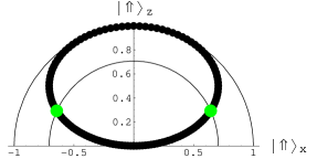
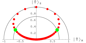
(a) (b) (c)

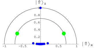
Figure 1: (Color online.) In the Figs.(a)-(c) the upper half of the $x$-plane of the Bloch sphere is plotted. The possible $\rho_{B}$’s and the nilpotent $v_{1}$ satisfying Eq. (30) form the ellipse given in Eq. (37). The dots in Fig.(a)/(b)/(c) represent the solution for the Bloch vectors for $\alpha_{1}=0/\frac{\pi}{3}/0.47\pi$, where $\phi_{1}$ varies $\in[-\frac{\pi}{2},\frac{\pi}{2}]$ with a step size $\pi/128$. For $\alpha_{1}=0$, Fig.(a), the solutions cover homogenously the ellipse and for $\alpha_{1}\rightarrow\pi/2$ they concentrate at the tracial state, i.e. there is an decrease of the set of possible solutions. For $\phi=0$ the pure spin up $|\Uparrow\rangle$ is always a solution. The two big (green) dots are the solutions for which the nearest neighbour entanglement maximizes, this is when the Bloch vector $|\vec{n}^{(\text{Bloch})}|=1/\sqrt{2}$ which is also plotted (inner half circle). For higher dimensions $b$ the absolute value of the generalized Bloch vector $\vec{n}^{(\text{Bloch})}$ is always around $\approx 1/\sqrt{2}$, see Table 1. Hence maximal entanglement between nearest neighbours is obtained if the “rest of the chain” is quite equally weighted in its purity and mixedness, measured by the squared length of the Bloch vector.

III.2.2 Properties of the nearest neighbour density matrix $\rho_{12}$

Let us now return to the original question, i.e. to the function that maximizes nearest neighbour entanglement. We have noticed in Sec.III.1 that due to the nilpotent choice of $v_{1}$ the trace of $\rho\tilde{\rho}$ gives only two non–vanishing eigenvalues, i.e. $\{A+|B|,A-|B|\}$. Concurrence of nearest entanglement for dimension $b=2$ is therefore

$${\cal C}(\rho_{12})\;=\;2\,{\rm Tr}(v_{2}^{\dagger}v_{1}^{\dagger}\,\rho_{B}\,v_{2}v_{1})=2\,\left|B\right|$$

$$=\frac{\cos^{2}\alpha_{1}\,\left(1+\sin\alpha_{1}\right)\,\sin^{2}\phi_{1}\,\cos^{2}\phi_{1}}{\cos^{2}\alpha_{1}\,\cos^{2}\phi_{1}\,\left(-1+\sin\alpha_{1}\right)-2\,\left(1+\sin\alpha_{1}\right)\,\sin^{2}\phi_{1}}\,,$$ (43)

and concurrence of assistance

$${\cal C}_{\text{ass}}(\rho_{12})\;=\;2\,{\rm Tr}(v_{1}^{\dagger}\,\rho_{B}\,v_{1})=2\,A$$

$$=\frac{\cos^{2}\alpha_{1}\,\left(1+\sin\alpha_{1}\right)\,\sin^{2}\phi_{1}}{\cos^{2}\alpha_{1}\,\cos^{2}\phi_{1}\,\left(-1+\sin\alpha_{1}\right)-2\,\left(1+\sin\alpha_{1}\right)\,\sin^{2}\phi_{1}}\,.$$ (44)

We have plotted both functions in Figure 2. One notices that while one can obtain for the concurrence of assistance all possible values, i.e. ${\cal C}_{\text{ass}}(\rho_{12})\in[0,1]$, concurrence of nearest neighbour entanglement has a maximum value of ${\cal C}_{\text{max}}(\rho_{12})=\sqrt{2}-1=0.41421$ for $\alpha_{1}=0.427079,\phi_{1}=0.571859$. This gives a concurrence of assistance of ${\cal C}_{\text{ass}}(\rho_{12})=0.585787$.

Further one notice that concurrences and concurrence of assistance are only equal for $\alpha_{1}$ or $\phi_{1}$ equal zero.

Armed with this analytical experience we proceed to the numerical procedure and present the results for increasing dimensionality $b$ of the auxiliary system.

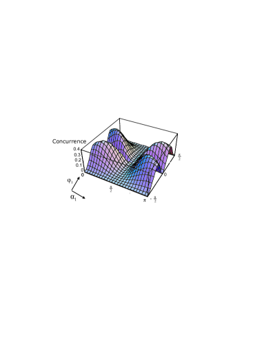
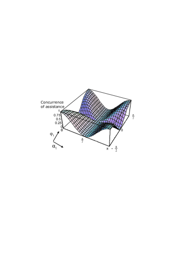
Figure 2: (Color online.) In Fig. (a) we have plotted the concurrence $\mathcal{C}_{12}(\rho_{12})$ of the nearest neighbour entanglement in Eq. (III.2.2) for the parameters $\alpha_{1}\in[0,\pi]$ and $\phi_{1}\in[-\frac{\pi}{2},\frac{\pi}{2}]$. The concurrence function is invariant under a shift of $\alpha_{1}$ with $\pi/2$ and $\phi\rightarrow-\phi$, thus we obtain four local maxima.
In Fig. (b) the concurrence of assistance $\mathcal{C}_{\text{ass}}(\rho_{12})$ in Eq. (III.2.2) is plotted. All possible values can be obtained.

All plotted quantities are dimensionless.

IV Numerical optimization of nearest neighbour entanglement

First we discuss the parametrization and our different strategies to numerically maximize nearest neighbour entanglement, then we discuss the results of the maximum in different dimensions $b$. Then we proceed with a discussion of the properties of such a chain maximizing nearest neighbour entanglement.

IV.1 Parametrization for dimension $b$

The triple $({\cal B},\mathbb{E},\rho_{B})$ defining the finitely correlated state is obtained by a finite number of parameters. We choose $\mathcal{B}={\bf M}_{b}$, and carry out calculations for different dimensionalities $b$. The completely positive map $\mathbb{E}$ is described by the two matrices $v_{1}$ and $v_{2}$ which are $b\times b$ matrices and have to satisfy the conditions Eq. (9, 10).

We choose $v_{1}$ to be a nilpotent operator as argued in the previous section, with a matrix of the form

$$v_{1}=\begin{pmatrix}0&&&\cr\cos(\alpha_{1})&0&&\cr&0&0&\cr&&\cos(\alpha_{2})&0\cr&&&0&0\cr&&&&\ddots&\ddots\end{pmatrix},$$ (45)

described by $[b/2]$ real parameters, $[\ldots]$ denoting the integer part. Though the parametrization is periodic with a periodicity of $2\pi$ in each parameter, the parameter values are unconstrained, which is an important simplification in the case of numerical optimization. In order to satisfy the unitality condition in Eq. (9), we set

$$v_{2}=\mathop{\mbox{diag}}\nolimits(1,\sin(\alpha_{1}),1,\sin(\alpha_{2}),\ldots)\,R,$$ (46)

where $R$ is an arbitrary $b\times b$ unitary matrix. However, according to our numerical experience for up to $b=6$ dimensions supports the conjecture that it is enough to consider real orthogonal matrices as $R$. The introduction of general unitary $R$-s did not lead to the increase of the maximal nearest neighbour concurrence. Thus we build up the generic $R\in SO(b)$ from rotations in two-dimensional subspaces, yielding the following (periodic, unconstrained) parametrization of $R$, with $b(b-1)/2$ parameters Murnaghan :

$$R = \begin{pmatrix}\cos(\phi_{1})&\sin(\phi_{1})&0&\ldots\cr-\sin(\phi_{1})&\cos(\phi_{1})&0&\ldots\cr 0&0&1&\ldots\cr\vdots&\vdots&\vdots&\ddots\end{pmatrix}\begin{pmatrix}\cos(\phi_{2})&0&\sin(\phi_{2})&\ldots\cr 0&1&0&\ldots\cr-\sin(\phi_{2})&0&\cos(\phi_{2})&\ldots\cr\vdots&\vdots&\vdots&\ddots\end{pmatrix}\ldots\begin{pmatrix}\cos(\phi_{b-1})&\ldots&\sin(\phi_{b-1})\cr 0&\ldots&0\cr\vdots&&\vdots&\cr-\sin(\phi_{b-1})&\ldots&\cos(\phi_{b-1})\end{pmatrix}$$ (47)

$$\times\begin{pmatrix}1&0&0&\ldots\cr 0&\cos(\phi_{b})&\sin(\phi_{b})&\ldots\cr 0&-\sin(\phi_{b})&\cos(\phi_{b})&\ldots\cr\vdots&&\vdots&\end{pmatrix}\ldots\begin{pmatrix}\ddots&&\vdots&\vdots\cr\ldots&1&0&0\cr\ldots&0&\cos(\phi_{b(b-1)/2})&\sin(\phi_{b(b-1)/2})\cr\ldots&0&-\sin(\phi_{b(b-1)/2})&\cos(\phi_{b(b-1)/2})\end{pmatrix}\,.$$

Thus given the dimensionality $b$, and a set of parameters $\underline{\alpha}=\alpha_{1}\ldots\alpha_{[b/2]}$, $\underline{\phi}=\phi_{1}\ldots\alpha_{b(b-1)/2}$, we can readily evaluate $v_{1}(\underline{\alpha})$ and $v_{2}(\underline{\alpha},\underline{\phi})$. Having these matrices at hand, we can calculate numerically $\rho$ from the translational invariance condition in Eq. (10). This can be done by noticing that Eq. (10) is linear in the matrix elements of $\rho$, thus we have to calculate the nullspace of the linear mapping

$$L(\rho)=\sum_{j=1}^{2}v_{j}^{\dagger}\ \rho\ v_{j}-\rho,$$ (48)

in the linear space of $b\times b$ matrices, in which all the vectors $\rho$ are suitable for our aims. We have found that for all the parameter settings arising in our optimization procedure $\mathop{\mbox{rank}}\nolimits L=b-1$ holds within the numerical precision, therefore the nullspace is one-dimensional. Hence for a fixed $b$ and parameters $\underline{\alpha},\underline{\phi}$, in addition to $v_{1}(\underline{\alpha})$ and $v_{2}(\underline{\alpha},\underline{\phi})$, we obtain a unique $\rho(\underline{\alpha},\underline{\phi})$. As a numerical check we verified that the solution is Hermitian positive semidefinite in all cases which have occurred.

Performing the above calculations we can compute the nearest-neighbour density matrix. From this density matrix we can evaluate the concurrence.

Thus for a fixed dimensionality $b$, we have a function $\mathcal{C}(\underline{\alpha},\underline{\phi})$ which we can numerically evaluate. This is the subject of an unconstrained numerical maximization in terms of its parameters. Unfortunately, it is not a convex function, thus there is no warranty to find a global maximum numerically. In addition the function might be not differentiable at certain points due to the properties of concurrence. Therefore we chose the simulated annealing method, which is known to be effective for mildly nonconvex and non-differentiable function. We have used the routines available in the MINTOOLKIT Creel04 package of GNU Octave software Octavemanual . First we have searched for the maximum using the samin routine, a simulated annealing code based on the implementation by Goffe Goffe96 . We have set the control parameters of the routine to $nt=20$, $ns=10$ $rt=0.75$, $neps=5$ and $eps=10^{-10}$ (consult the documentation Creel04 of the routine for their exact meaning). The routine showed a normal convergence in each case. Then the so-obtained maxima were used as an initial condition for a conjugate gradient search bfgsmin, with numerical gradient. We have found that the function is indeed differentiable around this maximum. The conjugate gradient search showed a strong convergence. The so obtainable final result is somewhat more accurate than the one obtained directly from simulated annealing. As a result of these procedure, we have obtained the parameter sets $\underline{\alpha},\underline{\phi}$ for which the nearest-neighbour concurrence $\mathcal{C}(\underline{\alpha},\underline{\phi})$ has a maximum value. Though this procedure does not give a full warranty for finding the global maximum, it is very likely that the obtained maxima are indeed global.

IV.2 Numerical results of the maximum nearest neighbour entanglement

We have summarized the results of the above described optimization procedure in Table 1. In case of entangled chains it is conjectured WoottersEntangledChains that the maximum value of nearest neighbour entanglement as measured by concurrence is ${\mathcal{C}_{W}}=0.434467$. As it is apparent from the results in Table 1, in our framework we can obtain a state which almost reaches this upper bound. Thus the translationally invariant finitely correlated chains can approach the state of an entangled chain with maximal bipartite entanglement quite fast. This is our main result. The approximation improves with the increasing dimensionality $b$ of the auxiliary Hilbert-space $\mathcal{B}$.

In addition, with accidental conjugate gradient searches we could obtain local maxima $\mathcal{C}=0.43406$ for $b=8$ and $\mathcal{C}=0.434095$ for $b=9$. These both constitute about $0.09\%$ relative difference from ${\mathcal{C}_{W}}=0.434467$.

We have to remark however, that as the maximum value of ${\mathcal{C}_{W}}$ is a conjecture, too, and we can neither fully warrant the global maximum, nor check the $b\to\infty$ case in the numerical framework, we cannot exclude the possibility to go beyond ${\mathcal{C}_{W}}$. Nevertheless we can prove explicitly that the bound can indeed be obtained in the framework of FCS, even under several restrictions.

Further we have checked numerically the possibility of using unitary instead of orthogonal matrices for $R$, and also the application of a more general, non-nilpotent $v_{1}$ by adding certain elements to its upper diagonal. We have found for $b$ up to $6$ that this does not improve the obtained maximal concurrence. In addition, the so arising $v_{1}$ was always nilpotent, with numerically the same matrix elements as in Eq. (45), though eventually ordered in a different form in the matrix. This supports the assumptions we have made as well as those in Ref. WoottersEntangledChains .

As we explicitly can calculate elements of the nearest neighbour state (see Table 2), we can ask which final state is approached for enlarging the dimensionality $b$ of the auxiliary system. For this we plotted the obtained nearest neighbour density matrices maximizing entanglement in a concurrence versus purity diagram (see Fig. 3). For dimension $b=9$ the relative difference of concurrence and purity of the nearest neighbour state maximizing entanglement and the maximally entangled mixed state (MEMS) Ref. IshizakaHiroshima , in our case $(\frac{1}{3}+\frac{1}{2}{\cal C}_{\text{W}})|\psi^{+}\rangle\langle\psi^{+}|+(\frac{1}{3}-\frac{1}{2}{\cal C}_{\text{W}})|\psi^{-}\rangle\langle\psi^{-}|+\frac{1}{3}|11\rangle\langle 11|$, is concerning concurrence $0.09\%$ and concerning purity $1.6\%$.

Dimensionality $b$	2	3	4	5	6	7
Nearest-neighbour concurrence	0.41421	0.41825	0.43200	0.43247	0.43336	0.43381
Relative difference
from Wootters’ bound (%)	4.66	3.73	0.57	0.46	0.25	0.15
$\alpha_{1}$	0.427079	3.27378	0.252679	6.345324	3.84312	2.71122
$\alpha_{2}$			2.888910	0.269592	0.10177	3.14860
$\alpha_{3}$					3.10541	3.29590
$\phi_{1}$	0.571859	3.14062	0.062823	6.22996	5.88873	6.27750
$\phi_{2}$		0.56623	5.504548	2.351162	6.10731	2.50188
$\phi_{3}$		4.17472	5.892460	2.713085	1.48352	3.33956
$\phi_{4}$			0.805037	0.047930	4.71882	6.25125
$\phi_{5}$			0.272233	5.137121	1.38430	5.62825
$\phi_{6}$			0.741237	0.417055	0.79196	3.76442
$\phi_{7}$				5.628356	4.81583	1.09039
$\phi_{8}$				1.759880	2.01345	3.43100
$\phi_{9}$				5.728579	0.306965	3.23516
$\phi_{10}$				1.193187	5.68444	2.87925
$\phi_{11}$					6.03621	4.95371
$\phi_{12}$					0.65283	0.28542
$\phi_{13}$					5.67111	1.87790
$\phi_{14}$					2.06680	5.46657
$\phi_{15}$					1.78624	1.14039
$\phi_{16}$						4.75900
$\phi_{17}$						2.68202
$\phi_{18}$						3.51887
$\phi_{19}$						5.54982
$\phi_{20}$						4.35086
$\phi_{21}$						0.478595

Table 1: Optimal nearest neighbour concurrences found in FCS, and the corresponding parameters

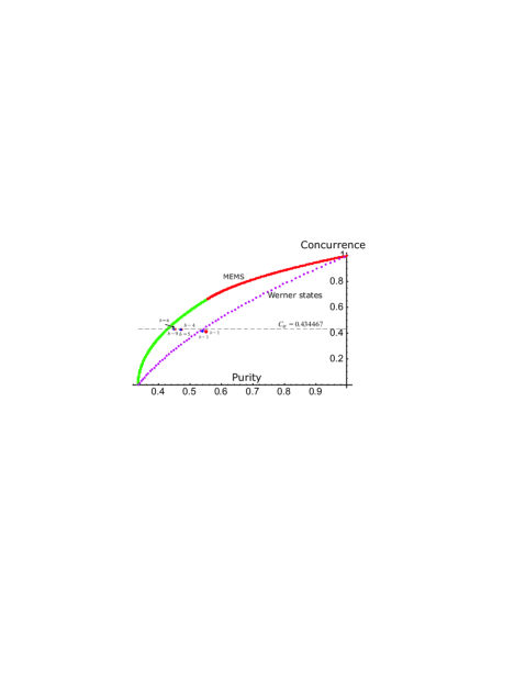
Figure 3: (Color online) Here concurrence versus purity measured by ${\rm Tr}\rho^{2}$ is plotted. The points below the curve represent all possible two-qubit density matrices. The curve itself are the maximally entangled mixed states (MEMS), first introduced in Ref. IshizakaHiroshima . The MEMS are defined up to local unitary transformations by $\rho^{\text{MEMS}}=(\frac{1}{3}+\frac{q}{2})|\psi^{+}\rangle\langle\psi^{+}|+(\frac{1}{3}-\frac{q}{2})|\psi^{-}\rangle\langle\psi^{-}|+\frac{1}{3}|11\rangle\langle 11|$ for $q\in[0,\frac{2}{3}]$ (green) and $\rho^{\text{MEMS}}=q|\psi^{+}\rangle\langle\psi^{+}|+(1-q)|11\rangle\langle 11|$ for $q\in[\frac{2}{3},1]$ (red). The dotted curve below (pink) are the density matrices of the isotropic states, the so–called Werner states $\rho_{\text{Werner}}=\frac{1-p}{4}\mathbbm{1}\otimes\mathbbm{1}+p\,|\psi^{+}\rangle\langle\psi^{+}|$. The horizontal dashed line represents all states having a concurrence of ${\cal C}_{\text{W}}=0.434467$. The dots are the nearest neighbour density matrices maximizing nearest neighbour entanglement where from left to right the dimensionality $b$ of the auxiliary system increases. One notices that the solutions seem to approach the bound of the realizable states, in particular the MEMS states. Further note that the picture of entanglement measure versus mixedness strongly depends on the chosen measure of entanglement and mixedness and that different entanglement measures define different ordering of states, see Ref. WeiKwiatVerstraete ; ZimanBuzek .

V Properties of the translational chain maximizing nearest entanglement

Let us investigate the question which properties an infinity translational chain has which maximizes nearest neighbour entanglement. Is the obtained chain like an ordinary bicycle chain (or Markov chain), whose links are only connected to two neighbouring links but not to the next and next–next neighbouring sites as our intuition may suggest?

Lets consider the state of three qubits in a line

$$\rho_{[1,3]} = \sum|s_{1}s_{2}s_{3}\rangle\langle t_{1}t_{2}t_{3}|\;Tr(v_{s_{1}}^{\dagger}v_{s_{2}}^{\dagger}v_{s_{3}}^{\dagger}\;\rho_{B}\;v_{t_{1}}v_{t_{2}}v_{t_{3}})$$

and tracing over qubit $2$ gives the density matrix for next nearest neighbours

$$\rho_{13} = Tr_{2}(\rho_{[1,3]})$$ (50)

$$= \sum|s_{1}s_{3}\rangle\langle t_{1}t_{3}|\left\{Tr(v_{s_{1}}^{\dagger}v_{1}^{\dagger}v_{s_{3}}^{\dagger}\rho_{B}\;v_{t_{1}}v_{1}v_{t_{3}})\right.$$

$$\left.\qquad\qquad\qquad+Tr(v_{s_{1}}^{\dagger}v_{2}^{\dagger}v_{s_{3}}^{\dagger}\rho_{B}\;v_{t_{1}}v_{2}v_{t_{3}})\right\}$$

If $v_{1}$ is nilpotent, this means that the first term of the the last equation vanishes (except of the last one but this has just to do with normalization). Thus it reduces the space dramatically in which we can vary. We checked that this next nearest neighbour entanglement for the parameters maximizing the nearest entanglement and found that it is zero for all auxiliary dimensions $b$. Thus we conclude that such a chain is an “ordinary bicycle chain”: only two neighbouring sites are linked via entanglement. Thisalso supports our assumption for a nilpotent generator because entanglement concentrates.

In Fig. 4 we plotted the concurrence and assisted concurrence for the dimension $b=2$ for different parameters. One sees that we can generally find parameters for which next nearest entanglement is nonzero, we checked the maximum possible concurrence available for our choice of generators, which is below the one of nearest neighbour entanglement ($C_{13}=0.169470$ for $\alpha_{1}=0.88563$ and $\phi_{1}=0.25066$ and a nearest neighbour concurrence of $C_{12}=0.270660$). When concurrence of next nearest neighbour entanglement increases then concurrence of assistance of next nearest neighbour entanglement decreases, as it is plotted in Fig.4 (b).

As the state of the whole chain is pure, we expect that purity has to increase considering the states of more and more qubits of the chain. We checked that for all considered cases, for example for $b=6$ $Tr\rho_{12}^{2}<Tr\rho_{123}^{2}$ is $0.452911<0.461722$ and for $b=9$ it changes to $0.447191<0.455342$, i.e. far away from $1$. Increasing dimensionality $b$ increases entanglement and also concentrates the correlation.

In Table 2 the relevant quantities are summarized. Notice that all quantities behave monotonically with increasing dimensionality $b$, except for the length of the Bloch vector. The fact that concurrence of assistance is bigger than concurrence suggest the presence of multipartite entanglement in the system.

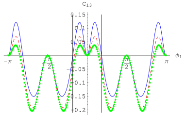
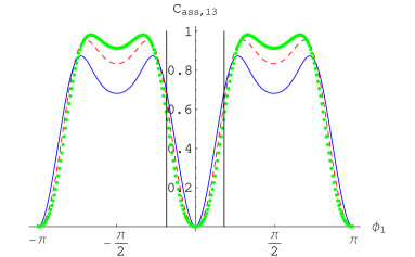
Figure 4: (Color online) (a) Here we plot $\mathcal{C}(\rho_{13})$ for $\alpha_{1}=0.6\text{ (blue)},0.42\text{ (red, dashed)},0.3\text{ (green, dotted)}$; the line is the maximizing $\phi_{1}=0.571859$ and the abscissa is $\phi_{1}\in[-\frac{\pi}{2},\frac{\pi}{2}]$. Note that we plotted $\lambda_{1}-\lambda_{2}$ while the concurrence is the maximum of $\{|\lambda_{1}-\lambda_{2}|,0\}$. (b) Here the concurrence of assistance $\mathcal{C}_{\text{ass}}=\rho_{13}$ for $\alpha_{1}=0.6\text{ (blue)},0.42\text{ (red, dashed)},0.3\text{ (green, dotted)}$ is plotted; abscissa $\phi_{1}\in[-\frac{\pi}{2},\frac{\pi}{2}]$. One notices when concurrence increases, concurrence of assistance decreases and vice versa.

Dimension b	2	3	4	5	6	9
${\cal C}_{\text{max}}(\rho_{12})$	$\;0.414214\;$	$\;0.41825\;$	$\;0.432000\;$	$\;0.432471\;$	$\;0.433791\;$	$\;0.434095\;$
${\cal C}_{\text{ass}}(\rho_{12})$	$0.585787$	$0.587251$	$0.600000$	$0.600131$	$0.601204$	$0.601442$
$\mathrm{A}$	0.292893	0.293626	0.300000	0.300066	0.300602	0.300721
$\mathrm{B}$	0.207107	0.209126	0.216000	0.216236	0.216895	0.217048
$\mathrm{C}$	0.174155	0.164125	0.097378	0.0925458	-0.069033	-0.0575684
Purity of ${\rm Tr}\rho_{12}^{2}$	0.550252	0.538009	0.471242	0.467748	0.452911	0.447191
Purity of ${\rm Tr}\rho_{1}^{2}$	0.646446	0.639055	0.598965	0.597077	0.58905	0.586052
$|\vec{n}^{(\text{Bloch})}|^{2}=\frac{b{\rm Tr}\rho_{B}^{2}-1}{b-1}$	0.5	0.607465	0.536326	0.554368	0.519502	0.521177

Table 2: Properties for different dimension $b$

VI Summary and conclusion

We have addressed the optimization of entanglement between nearest neighbours in an infinite translational invariant chain in an increasing set of states. Using finitely correlated states with a recursive structure and certain reasonable assumptions we have shown that the nearest neighbour entanglement almost reaches its conjectured upper bound $C_{\text{W}}=0.434467$. Our approach allows for an explicit calculation of the elements of the nearest neighbour density matrix maximizing entanglement. We show that in a concurrence versus purity (measured by $Tr\rho^{2}$) diagram the obtained nearest neighbour state seems to approach the maximally entangled mixed states (MEMS) which bound the realizable bipartite states in this diagram.

The approach we have adopted has the same roots as the DMRG methods. However, instead of using a matrix product form for a state of a finite set of qubits the formalism used provides an exact description of the infinite chain. The accuracy of the approximation increases with the dimensionality $b$ of the auxiliary Hilbert space.

For dimension $b=2$ and $b=3$ we have given a detailed analytical treatment of the problem while in higher dimensions we rely on numerical calculations. Apart from the investigation of nearest neighbour entanglement we have evaluated other properties of the chain. These results support the qualitative expectations that due to the monogamy of entanglement the increase in the nearest neighbour entanglement leads to the decrease in the longer distance quantum correlation. Not only concurrence but also the whole nearest neighbour density matrix tends to reach a given fixed value. This is, however, not the case with the state of the whole system. The difference of the concurrence and the concurrence of assistance suggest that some kind of multipartite entanglement is also present.

The variational technique utilized in our work may be applicable in other similar physical problems.

$$\lambda^{1}=\left(\begin{array}[]{ccc}0&1&0\\ 1&0&0\\ 0&0&0\\ \end{array}\right),\quad\lambda^{2}=\left(\begin{array}[]{ccc}0&-i&0\\ i&0&0\\ 0&0&0\\ \end{array}\right),$$

$$\lambda^{3}=\left(\begin{array}[]{ccc}1&0&0\\ 0&-1&0\\ 0&0&0\\ \end{array}\right),\quad\lambda^{4}=\left(\begin{array}[]{ccc}0&0&1\\ 0&0&0\\ 1&0&0\\ \end{array}\right),$$

$$\lambda^{5}=\left(\begin{array}[]{ccc}0&0&-i\\ 0&0&0\\ i&0&0\\ \end{array}\right),\quad\lambda^{6}=\left(\begin{array}[]{ccc}0&0&0\\ 0&0&1\\ 0&1&0\\ \end{array}\right),$$

$$\lambda^{7}=\left(\begin{array}[]{ccc}0&0&0\\ 0&0&-i\\ 0&i&0\\ \end{array}\right),\quad\lambda^{8}=\frac{1}{\sqrt{3}}\left(\begin{array}[]{ccc}1&0&0\\ 0&1&0\\ 0&0&-2\\ \end{array}\right)\,.$$

- (1) U. Schollwöck, Rev. Mod. Phys. 77, 259 (2005).
- (2) V. Coffman, J. Kundu, and W.K. Wootters, Phys. Rev. A 61, 052306 (2000).
- (3) T.J. Osborne and F. Verstraete, “General monogamy inequality for bipartite qubit entanglement”, e-print quant-ph/0502176.
- (4) M. Plesch and V. Bužek, Phys. Rev. A 67, 012322 (2003); M. Plesch, Z. Dzurákova, J. Novotný, and V. Bužek, J. Phys. A (Math. Gen.) 37, 1843-1859 (2004).
- (5) K.M. O’Connor, and W.K. Wootters, Phys. Rev. A 63, 052302 (2001).
- (6) J. I. Cirac and P. Zoller, Phys. Rev. Lett. 74, 4091 (1995).
- (7) W.K. Wootters, Contemporary Mathematics 305, 299 (2002).
- (8) M. Fannes, B. Nachtergaele, and R.F. Werner, Comm. Math. Phys. 144, 443 (1992); ibit, Europhys. Lett. 10, 633 (1989); ibit, J. Phys. A, Math. Gen. 24, L185 (1991).
- (9) F. Verstraete, D. Porras, and J. I. Cirac, Phys. Rev. Lett. 93 227205 (2004).
- (10) F. Benatti, B. C. Hiesmayr, and H. Narnhofer, Europhys. Lett. 72, 28 (2005).
- (11) F. Benatti, B. C. Hiesmayr, and H. Narnhofer, to be published in Journal of Laser Physics.
- (12) The authors of Ref. BHN1 ; BHN2 showed that there is a necessary condition for one qubit of the chain to be entangled with another qubit or other connected qubits. Namely, nearest-neighbours are entangled if the state of one qubit with the rest of the chain is entangled.
- (13) O. Bratteli and D.W. Robinson, Operators and Quantum Statistical Mechanics 2, Springer Berlin, 2nd ed. (1996).
- (14) M. Fannes, B. Nachtergaele, and R.F. Werner, Lett. Math. Phys. 25, 249 (1992).
- (15) S. Hill, and W.K. Wootters, Phys. Rev. Lett. 78, 5022 (1997); W.K. Wootters, Phys. Rev. Lett. 80, 2245 (1998).
- (16) W.K. Wootters, Phys. Rev. Lett. 80, 2245 (1998)
- (17) C.H. Bennett, D.P. DiVincenzo, J.A. Smolin, and W.K. Wootters, Phys. Rev. A 54, 3824 (1996).
- (18) D. P. DiVincenzo, C. A. Fuchs, H. Mabuchi, J. A. Smolin, Thapliyal, and A. Uhlmann, Quantum Computing and Quatum Communications, Lecture Notes in Computer Science, Vol. 1509 (Springer-Verlag, Berlin, 1999), p. 247.
- (19) T. Laustsen, F. Verstraete, and S. J. Van Enk, Quantum Inf. Comput. 3, 64 (2003).
- (20) F. D. Murnaghan, The Orthogonal and Symplectic Groups (Institute for Advanced Studies, Dublin, 1958).
- (21) M. Creel, UFAE and IAE Working Papers 607.04, Unitat de Fonaments de l’Anàlisi Econòmica (UAB) and Institut d’Anàlisi Econòmica (CSIC), available at http://ideas.repec.org/p/aub/autbar/607.04.html.
- (22) J. W. Eaton, GNU Octave manual (Network Theory Ltd., Bristol, United Kingdom, 2002).
- (23) W. Goffe, Studies in Nonlinear Dynamics & Econometrics 1, 169 (1996), available at http://ideas.repec.org/a/bep/sndecm/119963169-176.html.
- (24) S. Ishizaka and T. Hiroshima, Phys. Rev. A 62, 022310 (2000).
- (25) T.Ch. Wei, K. Nemoto, P.M. Goldbart, P.G. Kwiat, W.J. Munro, and F. Verstraete, Phys. Rev. A 67, 022110 (2003).
- (26) M. Ziman and V. Bužek, Phys. Rev. A 72, 052325 (2005).