Entanglement and quantum phase transitions

Abstract

We examine several well known quantum spin models and categorize behavior of pairwise entanglement at quantum phase transitions. A unified picture on the connection between the entanglement and quantum phase transition is given.

Quantum phase transitions (QPTs) at zero temperature are characterized by the change in the properties of the ground state of a many-body system caused by modifications in the interactions among its constituents Sachdev . QPTs are induced as a parameter $g$ in the system Hamiltonian $H(g)$ is varied across a point $g_{c}$. These phase transitions are completely driven by the quantum fluctuations and are incarnated via the non-analytic behaviors of the ground-state properties at the transition points. On the other hand, as it is well known, the concept of entanglement lies at the heart of quantum mechanics Einstein ; Schrodinger . Therefore, one expects that quantum entanglement (QE) should play an important role in QPTs. Recently, a great deal of effort has been devoted to understanding their connection. Indeed, it has been observed that the quantum phase transitions are signaled by critical behaviors of the concurrence, a measurement of bipartite entanglement WKWootters98 , in a number of spin models AOsterloh2002 ; TJOsbornee ; GVidal2003 ; SJGu03 ; OFSyljuasen03 ; SJGu05 ; JVidal04 ; JVidal042 ; LAWu04 ; MFYang05 ; SJGu04J1J2 . However, they are not universal. For example, for the transverse-field Ising model, Osterloh et. al. found that the first order derivative of the concurrence diverges at the transition point and obeys a scaling law in its vicinity AOsterloh2002 ; TJOsbornee . On the other hand, for the antiferromagnetic $XXZ$ chain (1D), the concurrence behaves in a completely different way. It is a continuous function of the anisotropic parameter and reaches its maximum at the transition point SJGu03 . While in two- and three-dimensional (2D & 3D) $XXZ$ modelsSJGu05 , it develops a cusp-like behavior around the critical point. Another interesting example is the so-called $J_{1}-J_{2}$ model (or Majumdar-Ghosh model) CKMajumdar69 . Its ground state undergoes a first-order phase transition at $J_{2}/J_{1}=0.5$ and a continuous phase transition at $J_{2}/J_{1}\simeq 0.241$. However, unlike the previous cases, the concurrence itself is now discontinuous at 0.5, while at 0.241, no discernable structure has been found SJGu04J1J2 . Therefore, a natural question arose is why the same quantity, which measures entanglement between two localized spins, has such different behaviors, such as singularityLAWu04 , maximum, scaling, etc., at QPTs? Further, is there a unified picture of QE at the QPT? Obviously, investigation on these issues will not only deepen our understanding in QPTs but also strengthen the connection between condensed matter physics and quantum information theory MANielsenb .

In this Letter, we study these issues by detail analysis of several well known spin models aim at giving a unified picture of QE at QPTs. For definiteness, we choose the concurrence, $C$, as the measure of pairwise entanglementWKWootters98 in this work. We characterize the behaviors of the concurrence into three types and emphasize the important role played by the low-lying excitation spectra reconstruction of many-body systems around the transition points in determining the critical behaviors of the concurrence. More precisely, we show that the low-lying excitation spectra of these models are reconstructed in three qualitatively different ways around $g_{c}$ and hence, their concurrences show the above-mentioned non-universal behaviors at the QPT points. Therefore, we are able to give a unified and intuitive picture to understand the relation between the QPT and the entanglement.

Table 1: The basic features of typical spin models, such as the properties of the concurrence, level-crossing(LC) in the ground-state (GS) and the first excited-state(ES), symmetry at the transition point, and type of phase transition.

Model (QPT point)	GS LC	ES LC	concurrence	symmetry	transition type	type
$XXZ$ chain($\Delta=-1$)	Yes		singular			I
$J_{1}-J_{2}$ model($J_{2}=0.5$)	Yes		singular			I
$XXZ$ chain($\Delta=1$)	No	Yes	maximum, not singular	SU(2) point	order-to-order	II
spin ladder($J=0$)	No	Yes	maximum, not singular	SU(2)$\otimes$SU(2)	disorder-to-disorder	II
$XXZ$ 2&3D($\Delta=1$)	No	Yes	maximum, singular	SU(2)	order-to-order	II
$J_{1}-J_{2}$ model($J_{2}\simeq 0.241$)	No	Yes	not maximum	unknown	order-to-disorder	III
Ising model($\lambda=1$)	No	No	singular, not maximum	unknown	disorder-to-order	III

To have concrete discussions, we concentrate on three well studied quantum spin models in one dimension, the $J_{1}-J_{2}$ model, the $XXZ$ model, and the transverse-field Ising model, defined by the following Hamiltonians:

$$\hat{H}_{\rm J_{1}-J_{2}} = \sum_{i}\left(J_{1}\hat{\bf s}_{i}\cdot\hat{\bf s}_{i+1}+J_{2}\hat{\bf s}_{i}\cdot\hat{\bf s}_{i+2}\right);$$ (1)

$$\hat{H}_{\rm XXZ} = \sum_{i}\left(\hat{s}_{i}^{x}\hat{s}_{i+1}^{x}+\hat{s}_{i}^{y}\hat{s}_{i+1}^{y}+\Delta\hat{s}_{i}^{z}\hat{s}_{i+1}^{z}\right);$$ (2)

$$\hat{H}_{\rm Ising} = -\sum_{i}\left(\lambda\hat{s}_{i}^{x}\hat{s}_{i+1}^{x}+\hat{s}_{i}^{z}/2\right).$$ (3)

In these Hamiltonians, $\hat{s}_{i}^{x},\>\hat{s}_{i}^{y}$ and $\hat{s}_{i}^{z}$ denote the spin operators at lattice site $i$. $J_{1},\>J_{2},\>\Delta$ and $\lambda>0$ are interaction parameters. The periodic boundary condition $\hat{s}_{1}=\hat{s}_{N+1}$ is assumed. In Table I, we present basic features of these three models. The concurrence of the $J_{1}-J_{2}$ model and the spin ladder is exemplified in Fig. 1, while the concurrence of the Ising model and the $XXZ$ model can be found in Refs. AOsterloh2002 ; TJOsbornee and Refs. SJGu03 ; OFSyljuasen03 ; SJGu05 respectively. As summarized in Table I, there exist three types of QE at QPT points: (I) $C$ is discontinuous; (II) $C$ is continuous and exhibits maximum at QPTs; (III) $C$ is continuous at QPTs but its higher order derivative exhibits extremum. We shall show that these seemingly different critical behaviors of the concurrence can be understood on the basis of the low-lying spectra reconstruction of these models around their QPT points. For this purpose, we present the ground-state energy and some low excited-state energies of the $J_{1}-J_{2}$ model, the $XXZ$ model, the spin ladder model and the transverse-field Ising model, on a finite chain in Fig. 2.

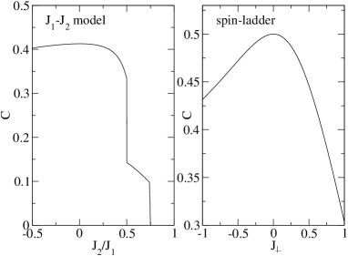
Figure 1: Concurrence of a 8-site $J_{1}-J_{2}$ model (LEFT) and a $2\times 4$ spin-ladder system (RIGHT).

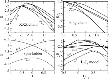
Figure 2: Low-lying energy spectra of four typical spin models.

For type I, we see immediately that, in both the $J_{1}-J_{2}$ and the $XXZ$ models, there exist ground-state level-crossing at $J_{2}/J_{1}=0.5$ and $\Delta=-1$, respectively. Since the concurrence is a measurement of bipartite entanglement in the ground state, it is not difficult to see why it changes discontinuously at these transition points. The same behavior was also observed in the first order transition in the spin model with mutual exchanges JVidal04 .

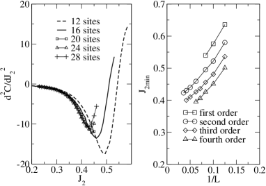
Figure 3: LEFT: The second derivative of the concurrence with respect to $J_{2}$ for various-size systems. RIGHT: The scale of the minimum point of the derivatives of the concurrence with different order.

To differentiate type II and III, we must take low-lying excitations into account. Let us study the spectra of the $XXZ$ model at $\Delta=1$, the spin ladder model at $J_{\perp}=0$, and the transverse-field Ising model at $\lambda=1$. It has been proven that the ground states of these models are nondegenerate around the corresponding transition points Lieb . At the first glance, it seems that this observation does not help us very much in understanding the critical behaviors of the concurrence in these models. However, as it is well known, QPTs are not solely dictated by the ground state of a specific model, especially on a finite system. They also depend on interconnection between the ground state and the low-lying excited states of the system Sachdev . In other words, the change of the ground-state properties is greatly affected by matrix elements of the relevant collective-mode operators, such as the spin-wave operators or the particle-density-wave operators, which relates the low-lying excited states to the ground state. In particular, in Ref. Tian03 , we pointed out that the QPT is actually induced by the reconstruction of the excitation energy spectra. As a consequence, when a transition takes place between two ordered phases of a system, such as the one for the $XXZ$ model at $\Delta=1$, which separates the $XY$ regime from the Ising regime, a level-crossing in its excited spectrum must occur. In fact, in Fig. 2, we see clearly the existence of such a level-crossing between the first and second excited states at $\Delta=1$ for the $XXZ$ model and at $J_{\perp}=0$ for the spin ladder model. Both excited states have total spin $S=1$ and are connected to the ground state, which is a spin singlet, via the spin-wave operators. It also implies that the system enjoys higher symmetries at the transition points. For instance, the $XXZ$ model has a $SU(2)$ symmetry at $\Delta=1$ while its symmetry group is weakened to $SU_{q}(2)$ for $\Delta\neq 1$. However, when the transition takes place between an ordered regime and a disordered one, the system remains gapless on the ordered side of the transition point and is gapful on the other side. Therefore, level-crossing of excited states is absent in this case. In our studies, the low-lying spectrum of the transverse-field Ising model has this character at $\lambda=1$.

On the other hand, the concurrence measures actually entanglement between two localized spins in a mixed state. Therefore, its behavior is also under the influence of the excited states of the system, especially the low-lying excited state. To see this point more clearly, let us first consider a generalized model in one dimension: $\hat{H}=\sum_{i}\left(J_{x}\hat{s}_{i}^{x}\hat{s}_{i+1}^{x}+J_{y}\hat{s}_{i}^{y}\hat{s}_{i+1}^{y}+J_{z}\hat{s}_{i}^{z}\hat{s}_{i+1}^{z}\right)+h\hat{s}_{i}^{z}$ which can be transformed into the 1D $XXZ$ model and the Ising model by appropriate choice of the parameters. We then introduce the identity: $\langle 0|[A,[H,A]]|0\rangle=2\sum_{n}(E_{n}-E_{0})|\langle 0|A|n\rangle|^{2}$, where $|n\rangle$ and $E_{n}$ denote the eigenstate and the corresponding eigenvalue. The choice of operator $A$ depends on the nature of local ordering. For the $XXZ$ model near $\Delta=1$, antiferromagnetic order dominates so we take $A=\hat{s}_{\pi}^{\alpha}=\sum_{j}e^{ij\pi}\hat{s}_{j}^{\alpha}$ and obtain

$$-\sum_{\alpha}\langle\hat{s}_{j}^{\alpha}\hat{s}_{j+1}^{\alpha}\rangle=\frac{E_{0}}{JN}+\frac{1}{NJ}\sum_{n\alpha}(E_{n}-E_{0})|\langle 0|\hat{s}_{\pi}^{\alpha}|n\rangle|^{2},$$ (4)

where $J=2+\Delta$. Obviously, the lhs of Eq. (4) is directly related to the concurrence of the $XXZ$ model $C=-2\sum_{\alpha}\langle\hat{s}_{j}^{\alpha}\hat{s}_{j+1}^{\alpha}\rangle-1/2$. While for the Ising model, the ferromagnetic order dominates so $A=\hat{s}_{0}^{\alpha}=\sum_{j}\hat{s}_{j}^{\alpha}$

$$\langle\hat{s}_{j}^{x}\hat{s}_{j+1}^{x}\rangle-\langle\hat{s}_{j}^{y}\hat{s}_{j+1}^{y}\rangle-\langle\hat{s}_{j}^{z}\hat{s}_{j+1}^{z}\rangle$$

$$=-\frac{E_{0}}{JN}-\frac{1}{NJ}\sum_{\alpha n}(E_{n}-E_{0})|\langle 0|\hat{s}_{0}^{\alpha}|n\rangle|^{2},$$ (5)

where $J=-\lambda$. The lhs of Eq. (5) is also directly related to the concurrence of the Ising model $C=2(\langle\hat{s}^{x}_{i}\hat{s}^{x}_{j}\rangle-\langle\hat{s}^{y}_{i}\hat{s}^{y}_{j}\rangle-\langle\hat{s}^{z}_{i}\hat{s}^{z}_{j}\rangle)-1/2$. The above two equations tell us that the concurrence does not simply depend on the re-scaled density of ground-state energy, but also the contributions from low-lying excited state with non-zero transition amplitude of the order operator to the ground state.

Keeping the above facts in mind, we now explain why the concurrence in the $XXZ$ model reaches its maximum at $\Delta=1$. Notice that, on the left-hand side of this point, the lowest excited states are doubly degenerate and have spin numbers $S=1,\>S_{z}=\pm 1$. Correspondingly, the matrix elements of spin operators $\hat{s}^{+}_{\pi}$ and $\hat{s}^{-}_{\pi}$ between them and the singlet ground state $|0\rangle$, are nonzero. On the other hand, the second excited state has spin number $S=1$ and $S_{z}=0$ and it contributes to the longitudinal spin correlation function. On the right-hand side of the transition point, these excited states interchange their position, as shown in Fig. 2. Since both sides are ordered phases, the main contributions to the corresponding order parameters are from the lowest excited state. Then the rhs of Eq. (4) can be written as $\frac{E_{0}}{JN}+\frac{1}{NJ}\sum_{\alpha}(E_{1}-E_{0})|\langle 0|\hat{s}_{\pi}^{\alpha}|1\rangle|^{2}$ approximately. Therefore, the main contribution to the concurrence is from transverse order operator in the $XY$ regime and from longitudinal order operator in Ising region. Only at the transition point $\Delta=1$, all three excited states have the same energy, and both the transverse and longitudinal spin correlation functions are power-law decay. Consequently, the contribution from both order operators to the concurrence makes it maximal.

However, the above argument for the $XXZ$ model is not valid for the transverse-field Ising model. For the latter, if $\lambda>1$, the ground state is ferromagnetic and has parity $P=1$, while the lowest excited has parity $P=-1$. So the rhs of Eq. (5) is mostly contributed from the first excited state and the decreasing of the concurrence as $\lambda$ increases can be well understood. When $\lambda$ approaches the critical point, the gap formation in the thermodynamic limit will introduce a significant change to the concurrence. This feature is reflected from the appearance of the minimum of the concurrence’s first derivative at the critical point. On the other hand, if $\lambda<1$, the phase is disordered and gapful. In this situation, though the matrix element of order parameter between the ground state and the first excited state becomes smaller and smaller, the second excited state and other higher excited state now can not be neglected. Their participation not only compensates the lose from the first excited, but also makes the concurrence to be maximal at one point. However, when $\lambda\rightarrow 0$, all excited state depart far away from the ground state which leads to the decrease of the concurrence. Finally, for the Ising model, its singular behavior around the critical point just results from the transition from paramagnetic phase to ferromagnetic long-range order phase as discussed in Refs. Sachdev ; SJGu05 .

With this understanding, let us take another look at the $J_{1}-J_{2}$ model. Besides the first-order transition point $J_{2}/J_{1}=0.5$, White and Affleck found a second-order transition at $J_{2}/J_{1}\sim 0.241$ by numerical calculation SRWhite96 . Around this point, the ground state of the model is nondegenerate but a level-crossing between two lowest excited states occurs as shown in Fig. 2. Again, a similar equation of the concurrence involving matrix element of antiferromagnetic order parameter can be obtained. Unlike the XXZ model at $\Delta=1$, one of the excited states involved in level-crossing is a spin singlet and all the matrix elements of spin operators between it and the ground state, which is also a spin singlet, are zero. Consequently, this exicted state does not affect the concurrence at all so the concurrence does not show a maximum around $J_{2}/J_{1}\sim 0.241$. Another excited state with spin $S=1$ involved in level-crossing is the only one who contributes to the concurrence significantly. Notice that this state is gapless for $J_{2}/J_{1}<0.241$ and is gapful otherwise. Therefore, the transition is actually of order-to-disorder type, which we observed in the transverse-field Ising model. In this case we expect that the critical behavior of the concurrence will show up in its higher-order derivatives. To check this statement, we show minimum of higher order derivatives of the concurrence as functions of system size in Fig. 3. Although lack of sufficient data for careful finite size scaling analysis makes it unclear one of the minima will tend to $J_{2}=0.241$, we believe that there exists a certain order derivative of the concurrence whose minimum will tend to 0.241 for an infinite system. Such behavior is consistent with our picture. On the other hand, the concurrence is quite flat in the ordered phase and has its maximum at $J_{2}/J_{1}=0$ (Fig. 1). This is due to the fact that the energy difference between the first excited state and the grounds state is almost a constant and the antiferromagnetic order parameter has its maximum at this point.

Finally, for type II and III, we argue that the singularity of the concurrence at the critical point arises from the change of the long-range order. First, if the system does not have long-range order, then local properties of the system, such as energy density, nearest-neighbor spin-spin correlation, etc., are not affected by spins far away, and their properties do not depend on the size of the system very much, nor does the concurrence. On the other hand, if the system has long-range order, the correlation function in momentum space will be $\delta$-function like, e.g., $F(g)\delta(q-\pi)$ for antiferromagnetic long-range order, where $F(g)$ is a coupling dependent function. Then the nearest-neighbor correlation function is, $\langle 0|\sigma^{\alpha}_{i}\sigma_{i+\delta}^{\alpha}|0\rangle\propto F(g)$. Thus, the change of long-range order at the critical point, e.g., from paramagnetic phase to magnetic order phase for the Ising model Sachdev , or from longitudinal magnetic order to that in the $xy$-plane for the 2D & 3D XXZ modelsXXZLRO , will obviously result in the change of $F(g)$ and leads to a singularity in the correlation function as well as the concurrence at the critical point. The size-dependent scaling behavior of the concurrence then comes naturally.

In summary, based on the properties of the low-lying excitation spectrum near the quantum transition points, we examined and classified the critical behaviors of the concurrence, a measure of pairwise entanglement, in several typical spin models. We show that discontinuity of the concurrence in $J_{1}-J_{2}$ model is simply caused by the ground-state level crossing at the transition point. On the other hand, QPT of the $XXZ$ model at $\Delta=1$ is of ordered-to-ordered type and hence, is accompanied by a level-crossing between its lowest excited states. Consequently, its concurrence has a maximum at the transition point. Finally, for the transverse-field Ising model, whose transition at $\lambda=1$ is of ordered-to-disordered type, the opening of energy gap at the transition point introduces an extremum to the high-order derivative of the concurrence. The singularity of the concurrence is the consequence of the transition of long-range-order. This classification gives a unified picture on the connection between the QE and QPTs.

This work is supported by RGC Projects CUHK 401703 and 401504 and by CNSF grant No. 90403003.

References

- (1) S. Sachdev, Quantum Phase Transitions, (Cambridge University Press, Cambridge, UK, 2000).
- (2) A. Einstein, B. Podolsky, and N. Rosen, Phys. Rev. 47, 777 (1935).
- (3) E. Schrödinger, Naturwissenschaften 23, 807 (1935).
- (4) W. K. Wootters, Phys. Rev. Lett. 80, 2245-2248 (1998); S. Hill and W. K. Wootters Phys. Rev. Lett. 78, 5022-5025 (1997).
- (5) A. Osterloh, Luigi Amico, G. Falci and Rosario Fazio, Nature 416, 608 (2002).
- (6) T. J. Osborne and M.A. Nielsen, Phys. Rev. A 66, 032110(2002).
- (7) G. Vidal, J. I. Latorre, E. Rico, and A. Kitaev, Phys. Rev. Lett. 90, 227902 (2003); J. I. Latorre, E. Rico, and G. Vidal, quant-ph/0304098 (2003).
- (8) S. J. Gu, H. Q. Lin, and Y. Q. Li, Phys. Rev. A 68, 042330 (2003).
- (9) Olav F. Syljuåsen Phys. Rev. A 68, 060301 (2003).
- (10) S. J. Gu, G. S. Tian, H. Q. Lin, Phys. Rev. A 71, 052322 (2005).
- (11) J. Vidal, G. Palacios, and R. Mosseri, Phys. Rev. A 69, 022107 (2004).
- (12) J. Vidal, R. Mosseri, J. Dukelsky, Phys. Rev. A 69, 054101 (2004).
- (13) L. A. Wu, M. S. Sarandy, and D. A. Lidar, Phys. Rev. Lett. 93, 250404 (2004).
- (14) M. F. Yang, Phys. Rev. A 71, 030302 (2005).
- (15) S. J. Gu, H. Li,Y. Q. Li, and H. Q. Lin, Phys. Rev. A 70, 052302 (2004); Recep Eryiğit, Resul Eryiğit, and Yiğit Gündüç, Int. J. Mod. Phys. C 15, 1095 (2004).
- (16) C.K. Majumdar and D.K. Ghosh, J. Math. Phys. 10, 1388 (1969).
- (17) M. A. Nielsen and I. L. Chuang, Quantum Computation and Quantum information (Cambridge University Press, Cambridge, 2000).
- (18) See for example, O. F. Syljuåsen1, S. Chakravarty, and M. Greven, Phys. Rev. Lett. 78, 4115 (1997).
- (19) E. Lieb and D. Mattis, J. Math. Phys. 3, 749 (1962).
- (20) G. S. Tian and H. Q. Lin, Phys. Rev. B 67, 245105 (2003).
- (21) S. R. White and I Affleck, Phys. Rev. B 54, 9862 (1996), and the references therein.
- (22) F. J. Dyson, E. H. Lieb, and B. Simon, J. Stat. Phys. 18, 335 (1978); T. Kennedy, E. Lieb, and B. S. Shastry, J. Stat. Phys. 53, 1019 (1988).