The electrodynamic 2-body problem
and the origin of quantum mechanics

C.K. Raju

Centre for Computer Science
MCRP University, Gyantantra Parisar
222, M.P. Nagar Zone I, Bhopal 462 011, India

Abstract

We numerically solve the functional differential equations (FDE’s) of 2-particle electrodynamics, using the full electrodynamic force obtained from the retarded Lienard-Wiechert potentials and the Lorentz force law. In contrast, the usual formulation uses only the Coulomb force (scalar potential), reducing the electrodynamic 2-body problem to a system of ordinary differential equations (ODE’s). The ODE formulation is mathematically suspect since FDE’s and ODE’s are known to be incompatible; however, the Coulomb approximation to the full electrodynamic force has been believed to be adequate for physics. We can now test this long-standing belief by comparing the FDE solution with the ODE solution, in the historically interesting case of the classical hydrogen atom. The solutions differ.

A key qualitative difference is that the full force involves a ‘delay’ torque. Our existing code is inadequate to calculate the detailed interaction of the delay torque with radiative damping. However, a symbolic calculation provides conditions under which the delay torque approximately balances (3rd order) radiative damping. Thus, further investigations are required, and it was prematurely concluded that radiative damping makes the classical hydrogen atom unstable. Solutions of FDE’s naturally exhibit an infinite spectrum of discrete frequencies. The conclusion is that (a) the Coulomb force is not a valid approximation to the full electrodynamic force, so that (b) the n-body interaction needs to be reformulated in various current contexts such as molecular dynamics.

pacs: 03.50.De, 03.30.+p, 02.30.Ks, 02.90.+p, 87.15.Aa, 31.15.-p, 03.65.Sq, 03.65.Ta, 95.35.+d

keywords: many-body problem, protein dynamics, functional differential equations, relativistic many-body problem, interpretation of quantum mechanics.

1 INTRODUCTION

1.1 Aim

This author had earlier⁽¹⁾ proposed a new model of time evolution in physics using mixed-type functional differential equations (FDE’s), with a tilt in the arrow of time. This paper sets aside the notion of a ‘tilt’, and takes up only the FDE’s of retarded electrodynamics. The retarded case already explicitly incorporates certain subtle mathematical features of electrodynamics and relativity noticed by Poincaré, but overlooked by Einstein and subsequent researchers. To bring out these subtleties, this paper reports on a numerically computed solution of FDE’s of the 2-body problem of classical retarded electrodynamics.⁽²⁾

The use of the full (retarded) electrodynamic 2-particle force leads to the formulation of the electrodynamic 2-body problem as a system of FDE’s that have not actually been solved earlier, numerically or otherwise, despite some sporadic attempts in simplified situations.⁽³⁾ In the absence of a systematic way to solve these FDE’s, a widely used alternative has been to approximate the full electrodynamic 2-particle force by the Coulomb force. This reformulates the electrodynamic 2-body problem as an easier system of ODE’s, which can be numerically solved with exactly the same numerical techniques that are used for the ODE’s of the classical 2-body problem of Newtonian gravitation. This alternative ODE formulation of the 2-particle electrodynamic interaction is incorporated, for example, in models of protein dynamics⁽⁴⁾ underlying current software such as charmm, wasser, amber etc.

This alternative ODE formulation is, however, mathematically suspect, for it is known that solutions of FDE’s may exhibit qualitative features impossible for solutions of ODE’s. On the other hand, it is believed that, from the viewpoint of physics, the Coulomb force is an adequate approximation to the full electrodynamic force.

We can now put this long-standing belief to test: our numerical solution of the full-force FDE’s enables us compare the two solutions in the historically interesting context of the classical hydrogen atom.

1.2 The full electrodynamic force

In classical electrodynamics, the force between moving charges is given by the Lienard-Wiechert potentials combined with the Heaviside-Lorentz force law. The scalar and vector (retarded) Lienard-Wiechert potentials, are given by the expressions⁽⁵⁾

$$V({\bf r},\>t)\>=\>{1\over 4\pi\epsilon_{0}}\>{qc\over(Rc-\>{\bf R\cdot v})}\>,\>\>\>\>{\bf A}({\bf r},\>t)\>=\>{{\bf v}\over c^{2}}V({\bf r},\>t).$$ (1)

One now computes the fields $\bf E$, and $\bf B$ by computing

$${\bf E}\>=\>-\nabla V\>-\>{\partial{\bf A}\over\partial t}\>,\quad{\bf B}\>=\>\nabla\>\times\>{\bf A}.$$ (2)

The expressions for these fields are:⁽⁶⁾

$${\bf E}\>=\>{q\over 4\pi\epsilon_{0}}\cdot{R\over({\bf R\cdot u})^{3}}\>\>[{\bf u}\>(c^{2}-v^{2})\>+\>{\bf R}\>\times\>({\bf u}\>\times\>{\bf a})],$$ (3)

$${\bf B}\>=\>{1\over c}{\bf\hat{R}}\times{\bf E}.$$ (4)

When these expressions for the fields $\bf E$, and $\bf B$ are substituted into the Heaviside-Lorentz force law,⁽⁷⁾

$${\bf F}\>=\>q_{1}\,\left({\bf E}\>+\>{\bf v}_{1}\times{\bf B}\,\right),$$ (5)

the force on a charge $q_{1}$ moving with velocity $v_{1}$ is given by the expression:⁽⁸⁾

$${\bf F}\> = \>{qq_{1}\over 4\pi\epsilon_{0}}{R\over(\bf R\cdot u)^{3}}\left\{\left[(c^{2}-v^{2}){\bf u}+{\bf R}\times(u\times a)\right]\right.$$ (6)

$${}+{{\bf v}_{1}\over c}\times\left.\left[{\bf\hat{R}}\times[(c^{2}-v^{2}){\bf u}+{\bf R}\times({\bf u}\times{\bf a})]\right]\right\}.$$

Here, charge $q_{1}$ is located at ${\bf r}(t)$ at time $t$, while the position of the other charge $q$ at time $t$ is given by ${\bf w}(t)$, and

$${\bf R}\>=\>{\bf r}(t)\>-\>{\bf w}(t_{r}).$$ (7)

In the above expression, $t_{r}$ is the retarded time (the time at which the backward null cone with vertex at ${\bf r}(t)$ meets the world line ${\bf w}(t)$ of the other charge), and is given implicitly by the equation

$$||{\bf r}(t)-{\bf w}(t_{r})||\>=\>c(t-t_{r}).$$ (8)

Further,

$${\bf u}\>=\>c{{\bf R}\over R}\>-\>{\bf v}\>=\>c{\bf\hat{R}}-{\bf v},$$ (9)

and it is understood that ${\bf v}\>=\>{\bf\dot{w}}(t_{r})$ and ${\bf a}\>=\>{\bf\ddot{w}}(t_{r})$ are the velocity and acceleration of the charge $q$ at the retarded time $t_{r}$. A similar expression gives the force exerted by the charge $q_{1}$ on the charge $q$. This leads to the formulation of the 2-body problem as a system of FDE’s.

1.3 The Coulomb approximation

An alternative formulation approximates the full force by the Coulomb force. This approximation has been justified as follows. In the Coulomb gauge, $\nabla\cdot{\bf A}\>=\>0$, the scalar potential $V$ satisfies the Poisson equation. Neglecting the vector potential, the force between the two particles (i.e., the force due to this scalar potential) is just the Coulomb force of electrostatics,

$${\bf F}\>=\>{qq_{1}\over r^{3}}{\bf r},$$ (10)

$\bf r$ being the instantaneous separation of the two particles. This leads to the formulation of the electrodynamic 2-body problem as a system of ODE’s, similar to the 2-particle ODE’s of Newtonian gravitation.

1.4 The difficulty: FDEs vs ODEs

However, the vector potential cannot be so easily neglected—the possible justification suggested above involves an all too facile analogy between the scalar Lienard-Wiechert potential and electrostatics. In the language of a text,

Don’t be fooled, though—unlike electrostatics, $V$ by itself doesn’t tell you $\bf E$, you need to know $\bf A$ as well.…$V$ by itself is not a physically measurable quantity—all the man in the moon can measure is $\bf E$, and that involves $\bf A$ as well. Somehow it is built into the vector potential, in the Coulomb gauge, that whereas $V$ instantaneously reflects all changes…$\bf E$ will change only after sufficient time has elapsed for the ‘news’ to arrive.⁽⁹⁾

Briefly, the Coulomb force (based on $V$) acts instantaneously, while the full force (based on $\bf E$) involves a delay (assuming retarded potentials).

Neglecting the vector potential, hence the delay, corresponds mathematically to approximating FDE’s by ODE’s. This is suspect since it is known that FDE’s are fundamentally different from ODE’s, and that solutions of FDE’s can have qualitative features impossible for solutions of ODE’s. The physical consequences of these differences are explained at length in the author’s previous book.⁽¹⁰⁾ Two differences of immediate concern are the following.

(a) Given a system of ODE’s of the form

$${\bf\dot{x}}(t)\>=\>g(t,\>{\bf x}(t))$$ (11)

a unique solution can be obtained by prescribing the initial values of $\bf{x}$ at a single point of time, say ${\bf x}(0)$. However, given a system of FDE ’s of the form

$${\bf\dot{x}}(t)\>=\>f\left(t,\>{\bf x}(t),\>{\bf x}(t-t_{r})\right)$$ (12)

and assuming these FDE’s to be retarded (i.e., $t_{r}>0$), this is no longer true. For example, consider the FDE

$$\dot{x}(t)\>=\>x(t-{\pi\over 2}).$$ (13)

Clearly, $x(t)\>=\>\sin(t)$ and $x(t)\>=\>\cos(t)$ are solutions, and since the equation is linear, any linear combination $x(t)\>=\>a\sin(t)\>+\>b\cos(t)$ is also a solution of (13), for arbitrary constants $a$ and $b$, and the values of both $a$ and $b$ obviously cannot be fixed from a knowledge of a single quantity $x(0)$.

In fact, from the mathematical theory of FDE’s,⁽¹¹⁾ it is known that prescribing the initial values of even an infinite number of derivatives, $x(0),~{}\dot{x}(0),~{}\ddot{x}(0)~{}\ldots$ is not adequate. To obtain a unique solution of the retarded FDE (12) we are required to prescribe the values of $x(t)$ over an entire interval $\left[0,\>-t_{r}\right]$, in the form of an initial function $\phi$. That is, to solve retarded FDE’s one needs to prescribe past data rather than instantaneous or ‘initial’(or final) data.

(b) Since the speed of light is so large, in many actual contexts, the delay $t_{r}$ is likely to be extremely small ($t_{r}<10^{-18}$s, for the classical hydrogen atom). Under these circumstances, it is tempting to approximate a FDE of the form (12) by an ODE of the form (11) by arguing that if the delay $t_{r}$ is small, then the values of $x(t-t_{r})$ can be approximately obtained from the values of $x(0)$, $\dot{x}(0)$, $\ddot{x}(0),\dddot{x}(0),\ldots$, by means of a ‘Taylor’ expansion. Such a procedure, however, is known to be erroneous because of fundamental qualitative differences between solutions of FDE’s and ODE’s. For example, unlike an ODE, which can be solved either forward or backward in time, a retarded FDE cannot generally be solved backward in time. Fig. 1 reproduced from Ref. 1 depicts ‘phase collapse’—three forward solutions of an FDE merge into one solution, so that a unique backward solution is impossible from data prescribed on the interval [1, 2]. Intersecting trajectories in phase space is a phenomenon impossible with ODE’s, so that the basic classical mechanics requirement of a phase flow breaks down.⁽¹²⁾ [The origin of this time-asymmetry is retrospectively obvious on physical grounds, since the force (6) has destroyed the underlying time symmetry of electrodynamics, by assuming retardation.]

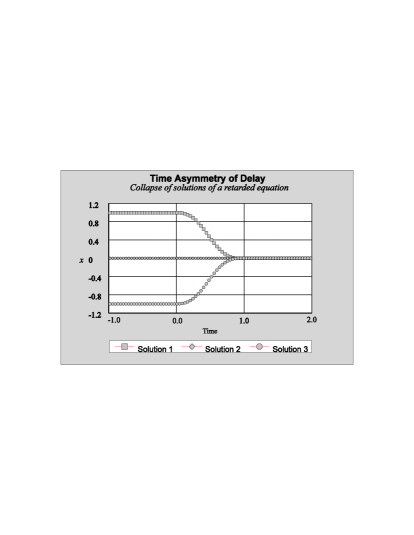
Figure 1: The figure shows three different solutions of a retarded FDE $\dot{x}(t)\>=\>b(t)x(t-1)$, for a suitable choice of the function $b(t)$. Three different past histories prescribed for $t\leq 0$ lead to three different solutions all of which coincide for $t\geq 1$. Such a phase collapse is impossible with ODE where trajectories in phase space can never intersect. Because of this phase collapse, FDE, unlike ODE, cannot be solved backward, from prescribed future data.

Thus, on grounds of the known mathematical differences between FDE’s and ODE’s, it is reasonable to doubt, a priori, that the full electrodynamic force (6) can be validly approximated by the Coulomb force, by neglecting the vector potential.

A good way to settle this doubt is to put the matter to test by comparing the Coulomb-force solution with the solutions obtained using the full electrodynamic force. This requires a solution of the 2-body problem with the full electrodynamic force, and we accordingly proceed to calculate such a solution.

2 SOLVING FDE’s

2.1 Method 1

The mathematical features of FDE’s briefly recapitulated above suggest that retarded electrodynamics involves a ‘paradigm shift’ from ‘classical mechanics’, for we now need past data rather than instantaneous data. In a debate on this question at Groningen, H. D. Zeh argued against any such paradigm shift. Zeh maintained that there was no need for past data, since data prescribed on a spacelike hypersurface (corresponding to an instant in spacetime) was adequate to solve the system of Maxwell’s partial differential equations (PDE’s) together with the Heaviside-Lorentz equations of motion for each particle.

Given all fields on a spacelike hypersurface, one can evolve them forward in time for a small region. Given all fields, in the vicinity of a single particle, its equations of motion reduce to a system of ODE’s which can be solved in the usual way. We will call this method 1. We note that it implicitly involves the simultaneous solution of a coupled system of PDE’s and ODE’s.

2.2 Method 2

In contrast to method 1, the FDE formulation of the electrodynamic 2-body problem may be geometrically visualised as follows.⁽¹³⁾ Assuming retarded potentials, the force on particle 1 at a given spacetime point $(a,\>0)$ is evaluated as follows. One constructs the backward null cone with vertex at $(a,\>0)$, and determines where it intersects the world-line of particle 2, at a point $(b,\>t)$, say (see Fig. 2). Given the world-line of the particle 2 in a neighborhood of $(b,\>t)$ one evaluates the resulting Lienard-Wiechert potential at $(a,\>0)$, and uses this retarded potential to calculate the force on particle 1 at $(a,\>0)$. This is the force given by (6). The force on particle 2 at any point is calculated similarly. Clearly, we can solve for the motion of either particle, only if we are given the appropriate portions of the past world line of the other particle. We will call this method 2.

2.3 Relating the two methods

The Groningen debate brought out the following difficulty. Both the above methods seem to have the same underlying physical principles (Newton’s laws of motion, possibly in a generalised form suitable for special relativity + Maxwell’s equations). How, then, can these principles admit fundamentally incompatible interpretations of instantaneity and history-dependence?

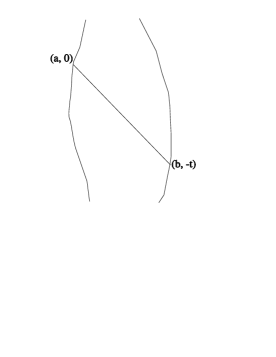
Figure 2: To calculate the force acting on particle 1 at $(a,0)$, one draws the backward null cone with vertex at $(a,0)$. If this intersects the world line of the second particle at $(b,-t)$, one calculates the Lienard-Wiechert potential at $(a,0)$, due to the motion of particle 2 at $(b,-t)$. Thus, determination of the present force on particle 1 requires a knowledge of the past motion of particle 2.

2.4 The need for past data

This issue can be readily resolved as follows. If retarded propagators (i.e., Green functions, or fundamental solutions of the wave equation, or retarded Lienard-Wiechert potentials) are assumed, then the field at any point $x$ relates to particle movements in the past at the points $x_{a}$ and $x_{b}$ on the respective world lines of particles $a$ and $b$, where the backward null cone from $x$ respectively meets the world lines of the two particles(Fig. 3). Thus, to know the field at a point x we should know the particle world lines at and around the past points $x_{a}$, and $x_{b}$. If we do this for every point $x$ on a spacelike hypersurface, the points $x_{a}$, and $x_{b}$ will, in general, cover the entire past world lines of the two particles. Thus, in the 2-body context, given the assumption of retardation, prescribing the fields on a spacelike hypersurface is really equivalent to prescribing the entire past histories of the two particles. That is,

instantaneous data for e.m. fields = past data for world lines of particles

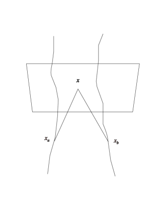
Figure 3: Method 1 seems to requires only instantaneous data corresponding to fields on a Cauchy hypersurface. Assuming only two particles and retarded propagators, the fields at any point $x$ on the hypersurface relate to past particle motions at $x_{a}$ and $x_{b}$. As $x$ runs over the hypersurface, the points $x_{a}$ and $x_{b}$ will, in general, cover the entire past. Thus, in the retarded case, initial data for the fields is the same as past data for the world lines of the particles.

That is, the PDE+ODE method 1 only hides the underlying history-dependence of electrodynamics. (The above remarks need to be appropriately modified if, instead of assuming retardation, one assumes advanced or mixed-type propagators. For example, if we use advanced propagators, then ‘anticipation’ should be used in place of ‘history-dependence’, etc.)

2.5 FDE vs ODE+PDE

While both methods require past data on the motion of the two particles, the intuitive schema underlying method 1 is currently inconvenient for the actual process of obtaining a solution. Formally speaking, there is no well-known existence and uniqueness theorem for a coupled system of PDE’s+ODE’s. [Separate existence theorems are, of course, known for PDE’s (Maxwell’s equations, in this case), and for ODE’s (to which the particle equations of motion reduce, if all fields are given).] Neither is there any well known numerical algorithm which converts the intuitive method of iteratively solving coupled PDE’s + ODE’s into an actual process of calculation.⁽¹⁴⁾ Both formal proof and a numerical scheme can very likely be developed without much difficulty. However, neither is available as of now, so method 1 cannot, as of now, be used to obtain a solution of the full-force electrodynamic 2-body problem.

In contrast, for FDE’s there already is a formal existence and uniqueness theorem from past data.⁽¹⁵⁾ Further, there are well known numerical algorithms and tested computer programs available⁽¹⁶⁾ (though they do not have all of the most desirable numerical characteristics, and the current code has not been formally proved to be error free). Accordingly, method 2 is currently the method of choice.

Incidentally, the PDE+ODE method 1 seems to need data on the entire past trajectories of the two particles. This is more information than is usually required for the FDE method 2. [Because of the numerical stiffness of the underlying equations, in practice, one is able to numerically solve the classical hydrogen atom with method 2 for only short time periods, of the order of a femto second ($10^{-15}$ s), for which only a very short portion of the past history is needed.] That is, method 1, despite its appearance of preserving instantaneity and not needing any information from the past, actually seems to need more information about the past than method 2! A very careful analysis of the method would presumably show that the solution by method 1 actually uses information from only that part of the Cauchy hypersurface within the Cauchy horizon, so that information across the entire hypersurface is not needed, and the two methods are really equivalent. At present, however, that is still a conjecture.

3 SOLUTION OF THE ELECTRODYNAMIC TWO-BODY PROBLEM

3.1 Prescription of past history and discontinuities

How should the past history of the two particles be prescribed? Existing physics provides no guidelines to help answer this question: exactly like fields on a spacelike hypersurface in method 1, it permits us to prescribe the past particle motions more or less arbitrarily.

This has two consequences worth noting. Thus, (1) mathematically, the past data for a FDE is not required to be a solution of the FDE, and (2) the mathematical theory of FDE’s tells us that a discontinuity may well develop at the initial point where the prescribed past data joins with the solution of the FDE.

From a physical point of view, this past motion may be regarded as a bound or constrained motion—constrained, perhaps, by additional mechanical forces—and the discontinuity at the initial point may be attributed to the sudden removal of the additional constraint at $t=0$. These discontinuities propagate downstream. While it is known from the general theory⁽¹⁷⁾ that the discontinuities of a retarded FDE are typically smoothened out over time, i.e., that they move over to successively higher derivatives, we must recognize that the problem we are solving is (except in 1 dimension) technically a neutral⁽¹⁸⁾ FDE (even though only retarded Lienard-Wiechert potentials are being used), so that no such smoothing need take place, and the discontinuities may persist.

The discontinuity creates a mathematical difficulty: for, in classical electrodynamics, the equations of motion are formulated assuming that the particle trajectories are at least thrice continuously differentiable ($C^{3}$). The numerical solution of the FDE by higher-order Runge-Kutta methods also assumes a similarly high level of smoothness, which assumption is not justified if the past history is prescribed arbitrarily.

This problem of discontinuities obviously is a suitable topic for further research, and in the sequel we shall set it aside and rely on the methods for handling discontinuities that are already incorporated into existing computer codes like retard and archi⁽¹⁹⁾, which handle discontinuities for example by switching to low-order polynomial extrapolation or predictor-corrector methods near a discontinuity. Both these programs are so written that they permit a discontinuity even in the function (positions, velocities) at the initial point, though we can always arrange initial conditions so that there is a discontinuity at most in the derivative (acceleration) at the initial point. We will prescribe past and initial data in such a way that discontinuities are confined to the acceleration and higher derivatives—though, like ‘quantum jumps’, it is not at present clear whether these are the only sorts of discontinuities that are ‘physically acceptable’. The archi program enables the tracking of such discontinuities, classified as ‘hard’ or ‘soft’ according to the theory of Willé and Baker.⁽²⁰⁾ Hard discontinuities are those that propagate instantaneously between components, while soft discontinuities are those that propagate over time. In the present context, since there are no advanced interactions, all discontinuities are soft, except for discontinuities between components (velocity, acceleration) representing derivatives. (Further, the archi program has certain refinements—such as the use of a cyclic queue to store past history—that are not immediately relevant.)

3.2 The classical hydrogen atom

To return to the physics, since our aim is to test how well the Coulomb force approximates the full electrodynamic force, let us consider the case of the classical hydrogen atom, without radiative damping. Suppose an electron and proton are for $t\leq 0$ constrained to rotate rigidly in a classical circular 2-body orbit, calculated using the Coulomb force. What will happen when this constraint is removed at $t=0$? With the past history prescribed in this way, we now have a complete problem that can be solved by method 2.

3.3 Equations of motion

That is, we take the non-relativistic equations of motion to be given by the Heaviside-Lorentz force law for each particle:⁽²¹⁾

$$m{d{\bf v}\over dt}\>=\>q\,\left({\bf E}\>+\>{\bf v}\times{\bf B}\,\right)\>\left[+{2\over 3}\,{q^{2}\over 4\pi\epsilon_{0}c^{3}}{d^{2}{\bf v}\over dt^{2}}\right].$$ (14)

The radiative damping term given by square brackets in (14) has been dropped, since it is not immediately relevant to our purpose of deciding whether the electrodynamic force (6) can be approximated by the Coulomb force. (We know that, in the absence of radiation damping, with the Coulomb force, the initial ‘Keplerian’ orbit should remain stable.) We also take the mass to be constant though, relativistically, only the proper mass is constant. This assumption, again, is appropriate to the comparison we wish to make between the Coulomb force and the full electrodynamic force.

3.4 Notation for the explicit system of equations

A slight change of notation is helpful for the explicit calculation. We let

$$\kappa\>=\>{q_{1}\,q_{2}\over 4\pi\epsilon_{0}m_{1}},\quad\mu\>=\>{m_{1}\over m_{2}}.$$ (15)

The mass ratio $\mu$ is dimensionless, while $\kappa$ has dimensions of $L^{3}T^{-2}$ (=length in units in which $c=1$). Denote the 3-dimensional trajectories of the two particles by ${\bf r}_{1}(t),\>{\bf r}_{2}(t)$. The delays $\tau,\>\bar{\tau}$ , and the vectors ${\bf R}_{1},\>{\bf R}_{2}$ are defined by the simultaneous equations

$$c^{2}\>\>~{}\tau^{2}\>=\>R_{1}^{2},\quad{\bf R}_{1}\>=\>{\bf r}_{2}(t)-{\bf r}_{1}(t-\tau),\quad R_{1}\>=\>||{\bf R}_{1}||,$$ (16)

$$c^{2}\>{\bar{\tau}}^{2}\>=\>R_{2}^{2},\quad{\bf R}_{2}\>=\>{\bf r}_{1}(t)-{\bf r}_{2}(t-\bar{\tau}),\quad R_{2}\>=\>||{\bf R}_{2}||.$$ (17)

Since here we consider only retarded solutions, for which $\tau,\bar{\tau}>0$ we need to solve only the equations

$$R_{1}-c\tau\>=\>0,$$ (18)

$$R_{2}-c\bar{\tau}\>=\>0,$$ (19)

to obtain $\tau,\>\bar{\tau}$ as functions of $t$, when suitable portions of the past trajectories ${\bf r}_{1}(t),\>{\bf r}_{2}(t)$ are known. Specifically, for each given $t$, we compute $\tau$ and $\bar{\tau}$ as the zeros of the functions $z_{1}(\tau)\equiv||r_{2}(t)-r_{1}(t-\tau)||-c\tau$, and $z_{2}(\bar{\tau})\equiv||r_{1}(t)-r_{2}(t-\bar{\tau})||-c\bar{\tau}$. The labelling has been chosen to make the equations below symmetrical.

We also introduce some notation to describe the velocity and acceleration at the retarded times:

$${\bf v}_{1}(t)\>=\>{d{\bf r}_{1}\over dt}(t),\quad{\bf v}_{1\,\mbox{r}}(t)\>=\>{\bf v}_{1}\,(t-\tau),\quad{\bf a}_{1\,\mbox{r}}(t)\>=\>{d{\bf v}_{1}\over dt}(t-\tau),$$ (20)

$${\bf v}_{2}(t)\>=\>{d{\bf r}_{2}\over dt}(t),\quad{\bf v}_{2\,\mbox{r}}(t)\>=\>{\bf v}_{2}\,(t-\bar{\tau}),\quad{\bf a}_{2\,\mbox{r}}(t)\>=\>{d{\bf v}_{2}\over dt}(t-\bar{\tau}).$$ (21)

For the vector $\bf u$ used to simplify the appearance of (6) we now have the expressions

$${\bf u}_{1}\>=\>c{\bf\hat{R}}_{1}\>-\>{\bf v}_{1\,\mbox{r}},\quad\mbox{and}\quad{\bf u}_{2}\>=\>c{\bf\hat{R}}_{2}\>-\>{\bf v}_{2\,\mbox{r}}.$$ (22)

With these notations, the equations of motion take the explicit form:

$${d{\bf v}_{1}\over dt}\>=\>\kappa\left[{\bf\tilde{E}}_{2}\>+\>{{\bf v}_{1}\over c}\times({\bf\hat{R}}_{2}\times{\bf\tilde{E}}_{2})\right],$$ (23)

$${d{\bf v}_{2}\over dt}\>=\>\mu\kappa\left[{\bf\tilde{E}}_{1}\>+\>{{\bf v}_{2}\over c}\times({\bf\hat{R}}_{1}\times{\bf\tilde{E}}_{1})\right],$$ (24)

where

$${\bf\tilde{E}}_{2}\>=\>{R_{2}\over({\bf R}_{2}\cdot{\bf u}_{2})^{3}}\>\>\left[{\bf u}_{2}\>(c^{2}-v_{2\,\mbox{r}}^{2})\>\>+\>\>{\bf R}_{2}\>\times\>({\bf u}_{2}\>\times\>{\bf a}_{2\,\mbox{r}})\right],$$ (25)

$${\bf\tilde{E}}_{1}\>=\>{R_{1}\over({\bf R}_{1}\cdot{\bf u}_{1})^{3}}\>\>\left[{\bf u}_{1}\>(c^{2}-v_{1\,\mbox{r}}^{2})\>\>+\>\>{\bf R}_{1}\>\times\>({\bf u}_{1}\>\times\>{\bf a}_{1\,\mbox{r}})\right].$$ (26)

The slight asymmetry between the two equations (23) and (24) is only apparent, but is helpful as follows. By convention we take the mass ratio $\mu\leq 1$, so the equation for the heavier particle is the one in which $\mu$ appears (and to calculate $\kappa$ we must use the mass of the lighter particle). For the purpose of computation we took $\mu$ as the mass ratio of the electron to the proton, and calculated $\kappa$ accordingly.

From the numerical point of view, the inverse of the mass ratio is a measure of the numerical stiffness of the problem. Thus, the problem is moderately stiff, and the numerical stiffness can be reduced by solving for a shorter time interval.

3.5 Actual system of equations to be solved numerically

The actual system of equations to be solved are the 12 retarded equations,

$$\dot{y}_{[i]}\>=\>f_{i}(t,y_{[i]},y_{[i]}(t-\tau)),$$ (27)

where

$$y_{[1]}\>=\>x_{1},\quad y_{[2]}\>=\>y_{1},\quad y_{[3]}\>=\>z_{1},$$ (28)

$$y_{[4]}\>=\>x_{2},\quad y_{[5]}\>=\>y_{2},\quad y_{[6]}\>=\>z_{2}.$$ (29)

$$y_{[7]}\>=\>v_{1x},\quad y_{[8]}\>=\>v_{1y},\quad y_{[9]}\>=\>v_{1z},$$ (30)

$$y_{[10]}\>=\>v_{2x},\quad y_{[11]}\>=\>v_{2y},\quad y_{[12]}\>=\>v_{2z}.$$ (31)

and ${\bf r}_{1}\>=\>(x_{1},\>y_{1},\>z_{1})$, ${\bf r}_{2}\>=\>(x_{2},\>y_{2},\>z_{2})$, ${\bf v}_{1}\>=\>(v_{1x},\>v_{1y},\>v_{1z})$ , ${\bf v}_{2}\>=\>(v_{2x},\>v_{2y},\>v_{2z})$.

Further,

$$\dot{y}_{[i]}\>=\>f_{i}\>\equiv\>y_{[i+6]}\quad\mbox{for}\>1\leq i\leq 6,$$ (32)

while for $7\leq i\leq 12$, the functions $f_{i}$ are to be computed using the equations of motion (14)–(26).

3.6 Initial functions

The past history is prescribed as rigid two-body rotation around a common centre of mass,

$${\bf r}_{1}(t)\>=\>r_{1}(\cos\,\omega t,\>\sin\,\omega t,0),$$ (33)

$${\bf{r}}_{2}(t)\>=\>r_{2}(\cos\>\omega t,\>\sin\>\omega t,0),$$ (34)

in a coordinate frame in which the centre of mass is fixed. From the definition of the centre of mass, $m_{1}r_{1}\>+m_{2}r_{2}\>=\>0$, so that $r_{e}/r_{p}\>=\>1/\mu$, with $r_{e}\>=\>r_{1}$ denoting the lighter particle according to the above convention for $\mu$. Thus, $r_{2}\>=\>-\mu r_{0}$. We took $r_{1}\>=\>r_{0}$ = classical atomic radius, and $\omega$ as the corresponding angular velocity required to balance the Coulomb force. We also need the past history of the velocities of the two particles, which is implicit in the above prescription. Explicitly,

$${\bf v}_{1}(t)\>=\>v_{1}(-\sin\,\omega t,\>\cos\,\omega t,0),$$ (35)

$${\bf v}_{2}(t)\>=\>v_{2}(-\sin\,\omega t,\>\cos\,\omega t,0),$$ (36)

with $v_{1}\>=\>\omega r_{1}$, $v_{2}\>=\>\omega r_{2}\>=\>-\mu v_{1}$.

3.7 Choice of units for computation

At this stage a new problem arises. The numerical values of the quantities we have proposed to use are as follows: $\mu\>=\>5.436\times 10^{-4}$, $\kappa\>=\>-2.528\times 10^{2}\>\mbox{m}^{3}\mbox{s}^{-2}$, $r_{0}\>=\>5.3\times 10^{-11}$ m, $v_{0}\>=\>\sqrt{\left({\kappa/r_{0}}\right)}$ = $2.18\times 10^{6}\>\mbox{ms}^{-1}$, $\omega\>=\>{v_{0}/r_{0}}\>=\>4.12\times 10^{16}\>\mbox{s}^{-1}$, $c\>=\>2.99\times 10^{8}\>\mbox{ms}^{-1}$. These numbers, spanning 27 orders of magnitude, present too wide a range for reliable practical computation.

This problem can be overcome by choosing computational units appropriately.The appropriate computational units are those in which all quantities are represented by numbers that are as close as possible to 1. Hence, the base SI units, or units in which $c=1$ are not the most appropriate, and it is preferable to take length in Angstroms or deci nano meters (1 dnm = $10^{-10}$ m) , and time in centi femto seconds (1 cfs = $10^{-17}$ s), so that the numerical values of the dimensioned quantities are as follows: $c\approx 30$ dnm/cfs, $\kappa\>=\>-0.02528$ (dnm)³ (cfs)^-2, $r_{0}\>=\>0.53$ dnm, $v_{0}\>=\>~{}0.218$ (dnm) (cfs)^-1, $\omega\>=\>0.412$ (cfs)^-1. The numbers now span only 3 orders of magnitude. This choice of computational units however means that the numerical solutions can be typically computed only for a few femto seconds. This is nevertheless adequate for our aims.

3.8 The solutions

The solutions were obtained using the retard program of Hairer et al.⁽²²⁾ The results of the numerical computation are shown in the accompanying figures. These results establish that it is faulty to use a model based on the balance of instantaneous forces in a circular orbit, with the Coulomb force as in the classical Kepler problem. If past history is prescribed on the basis of this model, for a proton-electron pair, the evolution takes place as shown on the right of the $y$-axes in Fig. 4. Though the difference is not immediately visible, it is substantial. The differences from the classically expected trajectory are shown in Figs. 5, 6. The differences are well outside the prescribed tolerances.

Figure 4: If the past history ($t<0$) is prescribed as a Keplerian orbit, then, in the absence of radiation damping, there is no visible change in the electron orbit for the classical hydrogen atom.

Figure 5: The time evolution of the difference from the classical orbit of the electron. Time is in centi femto seconds, and distances are in deci nano meters. The zero difference part corresponds to the prescribed past history. The difference that was not visible in the previous figure, is now seen to be large.

Figure 6: The time evolution of the difference of only the $x$-coordinate of the electron from its classical expectation. Same scale as before.

3.9 The delay torque

Apart from the purely numerical difference, there is a new qualitative feature. The full force acting on the electron has a tangential component along the direction of the electron velocity. Accordingly, it has a torque about the centre of mass, which torque initially accelerates the electron. With the Coulomb force, such a tangential component of force, or a torque, is clearly impossible: since the Coulomb force acts instantaneously, it always acts along the line through the instantaneous centre of mass. The time evolution of this torque is exhibited in Fig. 7. During the prescribed past history, this torque is a constant. Subsequently, it oscillates, so that the FDE solution oscillates about the ODE solution, and the entirety of the FDE orbit never strays very far from the entirety of the ODE orbit.

Figure 7: The plot shows the time variation in the tangential component of the force exerted by the proton on the electron. This component is constant during the prescribed past history of the rigid rotation. Subsequently, it oscillates. Thus, the electron is alternately accelerated and retarded.

4 HEURISTICS

4.1 The need for heuristics

Given the fundamental differences between FDE and ODE, it would have been astonishing if the above calculations had not shown up a difference from classical expectations. However, the above results are based on a mathematical theory, which, despite its rigor, is not commonly known to physicists. Further, the results of a complex numerical calculation might well involve some hidden error or subtle instability. Accordingly, one gains greater confidence in the numerical results if there is a way to understand the results intuitively and heuristically. This is not easy, given that the physicist’s intuition is trained around ODE’s, that are fundamentally different from the FDE’s used in the above calculation. However, we may proceed as follows.

4.2 The retarded inverse square force

For an intuitive understanding of the above result, we need to approximate the force (6) by a simpler force. Any instantaneous approximation, such as the Coulomb force, would be mathematically unsound. Nothing we know, however, prevents us from approximating an FDE by a simpler FDE. That is, we may well approximate the full electrodynamic force by a simpler force while retaining the delay.

Accordingly, let us consider a force which varies inversely as the square of the retarded distance. The retarded distance is the distance from the current position of the electron to the ‘last seen’ position of the proton (Fig. 8). Such a force is not physically acceptable, since it cannot be relativistically covariant; however, the simple expression for the force helps us to understand intuitively the consequences of a delay.

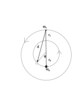
Figure 8: The figure shows two charged particles $e$ and $p$, with masses $m_{e}$ and $m_{p}$, rotating rigidly about a common centre of mass $C$, in circles of radii $r_{1}$ and $r_{2}$ respectively, with an assumed uniform angular velocity $\omega$. The classical force exerted by $p$ on $e$ acts along the line joining $e$ to the ‘last seen’ position of $p$, which differs from its instantaneous position by the delay angle $\theta\>=\>\omega\>\delta t$, where both $\delta t$ and $d$ are uniquely fixed by the condition $\delta t\>=\>d/c$, $c$ being the speed of light.

4.3 The delay torque

The key point here is not the exact magnitude of the force, but its direction: for this force acts along the line joining the current position of the electron to the last seen position of the proton. We can now immediately see the effect of even a tiny delay. Assume, to begin with, that the two particles are rotating rigidly in circular orbits about a common centre of mass. Because of the retardation, howsoever tiny, the last seen position of the proton can never be the same as its instantaneous position. Therefore, because of the retardation, howsoever tiny, the instantaneous force acting on the electron can not pass through the instantaneous centre of mass. The situation for the other charged particle is similar. These circumstances are anathema to classical mechanics, for it is a well known that, under such circumstances, angular momentum cannot be conserved. Thus, we have the astonishing situation that, purely under the action of internal forces, the system suffers a net torque.

The last seen position of the proton always lags behind its instantaneous position. Hence, for the situation of rigid rotation depicted in Fig. 8, the force exerted by the proton on the electron has a positive component in the direction of the electron velocity. Hence, the force tends to accelerate the electron.

We can use the retarded inverse-square force approximation also to heuristically try to understand the oscillation of the computed delay torque. The initial delay torque first accelerates both particles. The last-seen position of the proton starts moving towards and eventually falls on the instantaneous normal line to the curve being traced by the electron, so that the delay torque (about the instantaneous centre of rotation/curvature) is zero. The last-seen position of the other particle (proton) then moves ‘ahead’ of the instantaneous normal line to the curve traced by the electron, where ‘ahead’ and ‘behind’ is with respect to the direction in which the curve is being traced. The delay torque changes sign and starts decelerating the electron. If we neglect radiation damping, angular momentum is conserved on the average. This is similar to what the numerical computation with the full electrodynamic force showed.

4.4 Radiation damping and stability

There is an old argument to the effect that the introduction of radiation damping makes the classical hydrogen atom unstable. This argument is based on the Coulomb-force formulation of the electrodynamic 2-body problem. For the full electrodynamic force, the effect of introducing radiation reaction is no longer obvious, because of the existence of a delay torque which initially accelerates the electron.

There are three difficulties here. First the exact form of the radiation damping term is not quite clear. Dirac’s⁽²³⁾ argument that the 5th and higher-order terms are too complicated for ‘a simple thing like the electron’ is an interesting argument, but not entirely convincing. Secondly, this author has pointed out that Dirac’s derivation of radiation reaction approximates a FDE by a ODE using a ‘Taylor’ expansion in powers of the delay, and the mathematically suspect nature of this approximation is reinforced by the above calculation. Finally, putting in 3rd order radiation reaction may be expected to result in a numerically ill-conditioned problem, and appropriate codes for this are yet to be developed. (The dopri 4-5 code used implicitly in retard is not appropriate for stiff ODE’s.)

Since the issues involved are complex, it is helpful to have an initial estimate about the outcome of such a rigorous calculation. For the purposes of such an initial estimate, about the effect of radiation damping, we again use the simple heuristic case of the retarded inverse square force, to determine whether there can be a balance of forces between the delay torque and 3rd order radiation damping.

To this end, consider two particles interacting through the retarded inverse square force. The force on the electron exerted by the proton is given by

$${\bf F}\>=\>{e^{2}\over d^{3}}\>{\bf d}.$$ (37)

The force acts in the direction of the 3-vector $\bf d$ , along which the proton is ‘last seen’ by the electron. The 3-vector $\bf d$ may be represented by

$${\bf d}\>=\>{\bf r}_{p}(t-\delta t)\>-\>{\bf r}_{e}(t),$$ (38)

where ${\bf r}_{p}(t)$, and ${\bf r}_{e}(t)$ denote respectively the instantaneous position vectors of the proton and electron, respectively, at time $t$, and $\delta t$ is the delay, so that ${\bf r}_{p}(t-\delta t)$ is the ‘last seen’ position of the proton.

Assuming that the two particles are in rigid rotation with constant angular velocity $\omega$, and referring back to Fig. 8, we have, in 3-vector notation,

$${\bf r}_{e}\> = \>r_{1}[\cos\,\omega t\,{\bf\hat{\imath}}\>+\>\sin\,\omega t\,{\bf\hat{\jmath}}],$$ (39)

$$-{\bf r}_{p}(t-\delta t)\> = \>r_{2}[\cos\,\omega(t-\delta t)\,{\bf\hat{\imath}}\>+\>\sin\,\omega(t-\delta t)\,{\bf\hat{\jmath}}]$$ (41)

$$\approx r_{2}\,[\cos\,\omega t\>+\>\omega\delta t\>\sin\,\omega t]\,{\bf\hat{\imath}}\>$$

$${}+\>r_{2}\,[\sin\,\omega t\>-\>\omega\delta t\>\cos\,\omega t]\,{\bf\hat{\jmath}}\,,$$

assuming that $\omega\delta t$ is small. This last assumption is justified since, for classical rigid rotation, $\omega~{}=~{}{v_{0}/r}$ , while $\delta t~{}\sim~{}r/c$, so that $\omega\delta t~{}\sim~{}v_{0}/c~{}\sim~{}0.01$.

Hence, the delay torque on the electron is given by

$${\bf r}_{e}\,\times\>{\bf F}\>=\>{e^{2}\over d^{3}}\>{\bf r}_{e}\times{\bf d}\>=\>{e^{2}\over d^{3}}r_{1}r_{2}\,\omega\delta t\,{\bf\hat{k}}.$$ (42)

To a first approximation, we may use $d~{}\sim~{}r_{1}\>+\>r_{2}\>=\>(1\>+\>\epsilon)r_{1}$, where $\epsilon\>=\>{m_{e}/m_{p}}$, is the ratio of the electron to proton mass. Accordingly, $r_{1}r_{2}\>=\>\epsilon r_{1}^{2}$, and, further using $\delta t~{}\sim~{}{d/c}$, the expression for the delay torque simplifies to

$$T_{\mbox{delay}}\>=\>{e^{2}\over c}\cdot{\epsilon\over(1+\epsilon)^{2}}\,\cdot\,\omega\>{\bf\hat{k}}\>\>\approx\>{\epsilon e^{2}\over c}\omega{\bf\hat{k}}.$$ (43)

On the other hand, for the ‘average’ force due to (3rd order) radiation reaction, we have the well-known formula⁽²⁴⁾

$${\bf F}_{\mbox{rad}}\>=\>{\mu_{0}q^{2}\over 6\pi c}{\bf\dot{a}}_{e}\>=\>{1\over 4\pi\epsilon_{0}}\cdot{2\over 3}{q^{2}\over c^{3}}{\bf\dot{a}}_{e}\>=\>{2\over 3}{e^{2}\over c^{3}}{\bf\dot{a}}_{e}.$$ (44)

For the case under consideration,

$${\bf\dot{a}}_{e}\>=\>{d{\bf a}_{e}\over dt}\>=\>-\omega^{2}{\bf v}_{e}.$$ (45)

Hence, the torque due to radiation damping

$$T_{\mbox{rad }}\>=\>{\bf r}_{e}\>\times\>{\bf F}_{\mbox{rad}}\>=\>{2\over 3}{e^{2}\over c^{3}}\cdot\>-\omega^{2}\cdot{\bf r}_{e}\times\>{\bf v}_{e}\>=\>-\,\>{2\over 3}{e^{2}\over c^{3}}\,\omega^{3}\,r_{e}^{2}\,{\bf\hat{k}}.$$ (46)

The two torques are oppositely directed. Thus, a necessary condition for conservation of angular momentum is

$$T_{\mbox{delay}}\>+\>T_{\mbox{rad}}\>=\>0,$$ (47)

which gives

$${e^{2}\over c}\cdot{\epsilon\over(1+\epsilon)^{2}}\cdot\omega\>=\>{2\over 3}{e^{2}\over c^{3}}\>\cdot\omega^{3}r_{e}^{2},$$ (48)

or

$$\omega^{2}\>=\>{3\over 2}{\epsilon\over(1+\epsilon)^{2}}\cdot{c^{2}\over r_{e}^{2}}\>\approx\>{3\over 2}{\epsilon c^{2}\over r_{e}^{2}}.$$ (49)

Once the constraint of rigid rotation is removed, many such equilibrium solutions may well exist, with or without radiative damping.

We note, incidentally, this condition for conservation of angular momentum is quite different from the classical condition for balance of forces, which requires $\omega^{2}\>=\>e^{2}/r_{e}^{3}$. Both conditions can hold simultaneously only for one value of $r$ which is smaller than the Bohr radius.

Thus, further investigations are required to determine the exact effects of radiative damping, and it was prematurely concluded that radiative damping makes the classical hydrogen atom unstable.

4.5 Discrete spectrum and FDE’s

The discreteness of the observed hydrogen spectrum has been regarded as another compelling argument against classical electrodynamics. Solutions of FDE’s can, however, admit an infinite discrete spectrum.

Thus, for example, consider the retarded harmonic oscillator, given by the linear, second order, retarded FDE

$$\ddot{x}(t)\>=\>-x(t-1),$$ (50)

It is easy to see that a function of the form

$$x(t)\>=\>e^{z_{k}\,t},$$ (51)

for complex $z_{k}$, is a solution of the equation (50) if and only if $z_{k}$ is a solution of the quasi-polynomial equation

$$z^{2}e^{z}\>=\>-1.$$ (52)

It is equally easy to see that the quasi-polynomial equation (52) has infinitely many complex solutions $z_{k}\>=\>x_{k}\>\pm\>i\,y_{k}$, and it is known⁽²⁵⁾ that the roots are discrete, with no cluster point, and that the large magnitude roots are given asymptotically by the approximate expression

$$y_{k}\>=\>2k\pi\>+\>\epsilon_{1}(k),$$ (53)

$$x_{k}\>=\>-\ln\,y_{k}\>+\>\epsilon_{2}(k),$$ (54)

where $\epsilon_{1}(k)\>\rightarrow 0$, and $\epsilon_{2}(k)\>\rightarrow 0$ as $|z_{k}|\>\rightarrow\infty$.

(Had we dropped the retardation from (50), and applied the same procedure instead to the usual harmonic oscillator, given by the ODE $\ddot{x}(t)\>=\>-x(t)$, that would have led, in the well-known way, to a quadratic polynomial $z^{2}\>=\>-1$ with exactly one pair of complex conjugate roots: $i$, and $-i$.)

Since the equation (50) is linear, any linear combination of these infinitely many oscillatory solutions of the form (51) is again a solution. Setting aside questions of convergence, it is clear that any finite linear combination of the form

$$x(t)\>=\>\sum_{k=1}^{n}\>a_{k}\,e^{z_{k}\,t},$$ (55)

with $z_{k}$ given by (54), say, is also a solution of (50). That is, in physical terms, the retarded harmonic oscillator, governed by the simple linear FDE (50), exhibits an infinite spectrum of discrete frequencies. The general solution is a convergent linear combination of oscillations at an infinity of discrete (‘quantized’) frequencies. As in quantum mechanics, to determine a unique solution one needs to know an ‘initial’ function. If the initial function is prescribed arbitrarily, we can expect discontinuities.

The above considerations remain valid for any linear FDE with constant coefficients and constant delay.⁽²⁶⁾ The locally linear approximation⁽²⁷⁾ suggests that such ‘quantization’ is also to be expected for the non-linear FDE’s of the electrodynamic 2-body problem. [For the FDE (12) this approximation may be obtained simply by replacing $f$ by its first-order ‘Taylor’ expansion, and then freezing the values of the delays $t_{r}$, in a neighborhood of the point at which we want to approximate the solution.]

Mere discreteness of the spectrum does not, of course, mean that the FDE formulation, using retarded electrodynamics, will correctly reproduce the actual spectrum of the hydrogen atom. Equally, mere discreteness of the spectrum was not an adequate argument against the classical hydrogen atom, which was prematurely rejected on the basis of the ODE formulation of the 2-body problem of electrodynamics. Though a further investigation of FDE’s may still lead to a rejection of the classical hydrogen atom for the right reasons, it could, on the other hand, well help to clarify the ‘missing link’ between classical and quantum mechanics, as in the structured-time interpretation of quantum mechanics.⁽²⁸⁾

5 CONCLUSIONS

1. The Coulomb force is not a good approximation to the full electrodynamic force between moving charges.

2. The classical hydrogen atom was prematurely rejected on the basis of the ODE formulation of the electrodynamic 2-body problem.

3. The n-body problem involving electrodynamic interactions—as formulated, for example, in current software for molecular dynamics—needs to be reformulated using FDE’s.

5.1 Acknowledgments

The author is grateful to Profs G. C. Hegerfeldt (Göttingen), Huw Price (Sydney), David Atkinson (Groningen), H. D. Zeh (Heidelberg), Dennis Dieks (Utrecht), Jos Uffink (Utrecht), C. J. S. Clarke (Southampton), P. T. Landsberg (Southampton), Amitabh Mukherjee (Delhi), and Mr Suvrat Raju (Harvard) for discussions, and to an anonymous referee for comments that have greatly helped to improve the presentation of the paper.

NOTES AND REFERENCES

1. C. K. Raju, Time: Towards a Consistent Theory, Kluwer Academic, Dordrecht, 1994. (Fundamental Theories of Physics, vol. 65.)

2. Preliminary versions of aspects of this paper have been circulating for some time, having been presented and discussed at various conferences and lectures over the past several years, e.g. “Simulating a tilt in the arrow of time: preliminary results,” Seminar on Some Aspects of Theoretical Physics, Indian Statistical Institute, Calcutta, 14–15 May 1996, “The electrodynamic 2–body problem and the origin of quantum mechanics.” Paper presented at the International Symposium on Uncertain Reality, New Delhi, 5–9 Jan 1998, “Relativity: history and history dependence.” Paper presented at the On Time Seminar, British Society for History of Science, and Royal Society for History of Science, Liverpool, August 1999. “Time travel,” invited talk at the International Seminar, Retrocausality Day, University of Groningen, September 1999, and in talks at the Universities of Southampton, Utrecht, Pittsburgh, etc.

3. Some attempts have been made to study the 2-body problem in 1 and 2-dimensions, and some approximation procedures have been suggested for three dimensions, but none of these are critically relevant to the question at hand. For a quick review see C. K. Raju, “Electromagnetic Time,” chp. 5b in Time: Towards a Consistent Theory, cited earlier. For the 1-body problem see C. F. Eliezer, Rev. Mod. Phys. 19 (1947) p. 147 ; G. N. Plass, Rev. Mod. Phys. 33, (1961) pp. 37–62. For the 2-body problem, see J. L. Synge, Proc. R. Soc. A177 (1940) pp. 118–139, R. D. Driver, Phys. Rev. 178 (1969) pp. 2051–57, D. K. Hsing, Phys. Rev. D16 (1977) pp. 974–82, A. Schild, Phys. Rev. 131 (1963) p. 2762, C. M Anderssen and H. C. von Baeyer, Phys. Rev. D5 (1972) p. , 802, Phys. Rev. D5 (1972) p. 2470, R. D. Driver, Phys. Rev. D19 (1979) p. 1098, L. S. Schulman, J. Math. Phys. 15 (1974) pp. 205–8, K. L. Cooke and D. W. Krumme, J. Math. Anal. Appl. 24 (1968) pp. 372–87, H. Van Dam and E. P. Wigner, Phys. Rev. 138B (1965) p. 1576, 142 (1966) p. 838.

4. J. Andrew McCammon and Stephen C. Harvey, Dynamics of Proteins and Nucleic Acids, Cambridge University Press, 1987, p. 61.

5. David J. Griffiths, Introduction to Electrodynamics, Prentice Hall, India, 3rd ed., 1999, p. 435, eq. 10.46. Cf. J. D. Jackson, Classical Electrodynamics, 3rd ed., John Wiley, 2001. Griffiths’ book is more convenient for our purpose.

6. cf. Griffiths, Electrodynamics, 3rd ed., equns. 10.65, 10.66 and 10.67, pp. 438–39.

7. usually called just the Lorentz force law.

8. Griffiths, Electrodynamics, 3rd ed., p. 439, eq. 10.67.

9. Griffiths, Electrodynamics, 3rd ed., p. 421. O. L. Brill and B. Goodman, Amer. J. Phys. 35, 1967, p. 832.

10. C. K. Raju, “Electromagnetic Time,” chp. 5b in Time: Towards a Consistent Theory, cited earlier.

11. L. E. El’sgol’tz, Introduction to the Theory of Differential Equations with Deviating Arguments, trans. R. J. McLaughlin, Holden-Day, San Francisco, 1966, pp. 13–19. R. D. Driver, Introduction to Differential and Delay Equations, Springer, Berlin, 1977.

12. C. K. Raju, “Electromagnetic Time,” chp. 5b in Time: Towards a Consistent Theory, cited earlier.

13. C. K. Raju, Time: Towards a Consistent Theory, cited earlier.

14. An earlier method suggested by Synge also assumes instantaneity, but it has the advantage that it can actually be implemented. This implementation will be considered in subsequent articles. See, J. L. Synge, “The electrodynamic 2-body problem,” J. R. Soc. A177 (1940) pp. 118–139.

15. El’sgol’tz, Differential Equations with Deviating Arguments, pp. 13–19. Driver, Differential and Delay Equations.

16. E. Hairer, S. P. Norsett, and G. Wanner, Solving Ordinary Differential Equations, Springer Series in Computational Mathematics, Vol. 8, Springer, Berlin, 1987. Revised ed. 1991.

17. El’sgol’ts, Differential Equations with Deviating Arguments, p. 9.

18. Driver, Differential and Delay Equations.

19. C. A. H. Paul, “A user guide to archi: an explicit Runge-Kutta code for solving delay and neutral differential equations,” Numerical Analysis Report No. 283, Department of Mathematics, University of Manchester, 1995.

20. D. R. Willé and C. T. H. Baker, “The tracking of derivative discontinuities in systems of delay differential equations,” Appl. Num. Math. 9 (1992) pp. 209–222.

21. Griffiths, Electrodynamics, 3rd ed., equns. 7.40, and 11.80, pp. 326 and 467.

22. E. Hairer, S. P. Norsett, and G. Wanner, Solving Ordinary Differential Equations, cited above. (The above figures used the newer version of retard.)

23. P. A. M. Dirac, “Classical theory of the radiating electron,” Proc. R. Soc. A 167 (1938) p. 148. Also F. Rohrlich, Classical Charged Particles, Addison-Wesley, Reading, Mass, 1985, p. 142.

24. Griffiths, Electrodynamics, 3rd ed., § 11.80, p. 467.

25. El’sgol’tz, Differential Equations with Deviating Arguments, pp. 32–33.

26. El’sgol’tz, Differential Equations with Deviating Arguments, pp. 28–41.

27. C. K. Raju, “Simulating a tilt in the arrow of time,” cited earlier. Such an approximation is a priori plausible, though there is, at present, no formal proof of its validity.

28. C. K. Raju, “Quantum-Mechanical Time,” chp. 6 in Time: Towards a Consistent Theory, cited earlier.