Semiquantum versus semiclassical mechanics for simple nonlinear systems

Quantum mechanics has been formulated in phase space, with the Wigner function as the representative of the quantum density operator, and classical mechanics has been formulated in Hilbert space, with the Groenewold operator as the representative of the classical Liouville density function. Semiclassical approximations to the quantum evolution of the Wigner function have been defined, enabling the quantum evolution to be approached from a classical starting point. Now analogous semiquantum approximations to the classical evolution of the Groenewold operator are defined, enabling the classical evolution to be approached from a quantum starting point. Simple nonlinear systems with one degree of freedom are considered, whose Hamiltonians are polynomials in the Hamiltonian of the simple harmonic oscillator. The behaviour of expectation values of simple observables and of eigenvalues of the Groenewold operator, are calculated numerically and compared for the various semiclassical and semiquantum approximations.

1 Introduction

Developments in nanotechnology have focussed increasing attention on the interface between quantum mechanics and classical mechanics. Since the earliest days of the quantum theory, the nature of this interface has been explored by means of various semiclassical approximations with the introduction of quantum corrections to classical behaviour, characterised by expansions of quantities of interest in asymptotic series in increasing powers of Planck’s constant $\hbar$ ; see for example [1, 2, 3, 4]. One such approach focusses on Wigner’s quasiprobability density, which is the representative of the quantum density operator in the formulation of quantum mechanics on phase space, and considers quantum corrections to the classical Liouvillean evolution. This approach has its roots in Wigner’s paper [1] where the quasiprobability function was first introduced, and it has recently been developed in some theoretical detail by Osborn and Molzahn [4], working in the Heisenberg picture.

Recently an alternative approach has been suggested, which we refer to as semiquantum mechanics [5]. This considers the quantum-classical interface from the other side, that is to say, from the quantum side. The idea is to consider a series of classical corrections to quantum mechanics, again characterised by increasing powers of $\hbar$. To facilitate this, we first reformulate classical mechanics, representing classical observables on phase space by hermitian operators on Hilbert space [6], and in particular representing the Liouville density by a quasidensity operator [7, 8, 5] (the Groenewold operator). This has many of the properties of a true density operator but is not positive-definite in general [9]. It is the analogue in the Hilbert space formulation of classical mechanics, of the Wigner function in the phase space formulation of quantum mechanics.

The evolution in time of the Groenewold operator corresponds to the classical evolution of the Liouville density, and has been given in [5] as a series of terms in increasing powers of $\hbar$, with the first term corresponding to the familiar quantum evolution. It is consideration of these terms successively that defines a series of approximations to classical dynamics, starting with quantum dynamics at the lowest order, and hence defining what we mean by semiquantum mechanics.

In what follows, we shall apply these ideas to some very simple nonlinear systems in one dimension. These are necessarily integrable, and so incapable of showing interesting dynamical behaviour such as chaos. However the nonlinearity provides a preliminary testing ground for semiquantum mechanics, as we consider successive classical corrections to the quantum dynamics, and see how the classical behaviour of expectation values of key observables emerges. We are able to identify some differences between semiquantum and semiclassical approximations at the interface between quantum and classical behaviours.

2 Semiquantum mechanics

The formulation of quantum mechanics in phase space is determined with the help of the unitary Weyl-Wigner transform ${\cal W}$, which maps each quantum observable (hermitian operator) ${\hat{A}}$ on Hilbert space into a real-valued function $A$ on phase space. In the case of one degree of freedom, and when ${\hat{A}}$ is regarded as an integral operator with kernel $A_{K}(x,y)$ in the coordinate representation, the action of ${\cal W}$ is defined by [10, 11, 12]

$$A(q,\,p)={\cal W}({\hat{A}})(q,\,p)=\int A_{K}(q-x/2,\,q+x/2)\,e^{ipx/\hbar}\,dx\,.$$ (1)

In the particular case of the density operator ${\hat{\rho}}$, we obtain the Wigner function

$$W(q,\,p)={\cal W}({\hat{\rho}}/2\pi\hbar)(q,\,p)\,.$$ (2)

Conversely, the formulation of classical mechanics in Hilbert space has been defined [6, 5] using the inverse transform ${\cal W}^{-1}$, which is Weyl’s quantization map. This acts on a classical observable (a real-valued function on phase space) $A$ to produce an hermitian operator ${\hat{A}}={\cal W}^{-1}(A)$ with kernel $A_{K}$ given by

$$A_{K}(x,y)={\cal W}^{-1}(A)_{K}(x,y)=\frac{1}{2\pi\hbar}\int A([x+y]/2,\,p)\,e^{ip(x-y)/\hbar}\,dp\,.$$ (3)

Typically ${\cal W}^{-1}$ is used only to establish the quantization of a given classical system. However, we can if we wish use it to map all of classical mechanics, including classical dynamics, into a Hilbert space formulation [6, 5]. Then $\hbar$ in (3) can be thought of as an arbitrary constant with dimensions of action [8], to be equated with Planck’s constant if and when desired.

Given a Liouville probability density on phase space, that is to say a function $\rho(q,\,p)$ satisfying

$$\int\rho(q,\,p)\,dq\,dp=1\,,\quad\rho(q,\,p)\geq 0\,,$$ (4)

we define the corresponding hermitian (integral) operator ${\hat{G}}={\cal W}^{-1}(2\pi\hbar\rho)$ using (3). This operator ${\hat{G}}$ is the Groenewold operator, which has all the properties of a true density operator except that it is not in general positive-definite. Thus if ${\hat{A}}={\cal W}^{-1}(A)$, then

$${\rm Tr}({\hat{G}})=1\,,\qquad{\rm Tr}({\hat{G}}\,^{2})\leq 1\,,\qquad\qquad$$

$$\langle A\rangle=\int\rho(q,\,p)\,A(q,\,p)\,dq\,dp=\langle{\hat{A}}\rangle={\rm Tr}({\hat{G}}{\hat{A}})\,,$$ (5)

but not all eigenvalues of ${\hat{G}}$ need be positive.

It was shown in [5] that for suitably smooth Hamiltonians, the classical time evolution of the Liouville density,

$$\partial\rho/\partial t=\rho_{q}H_{p}-\rho_{p}H_{q}$$ (6)

is mapped into the evolution

$$\frac{\partial{\hat{G}}(t)}{\partial t}=\frac{1}{i\hbar}[{\hat{H}},{\hat{G}}]-\frac{i\hbar}{24}\left([{\hat{H}}_{qq},\,{\hat{G}}_{pp}]-2[{\hat{H}}_{qp},\,{\hat{G}}_{qp}]+[{\hat{H}}_{pp},\,{\hat{G}}_{qq}]\right)$$

$$-\frac{7i\hbar^{3}}{5760}\left([{\hat{H}}_{qqqq},\,{\hat{G}}_{pppp}]-4[{\hat{H}}_{qqqp},\,{\hat{G}}_{qppp}]+6[{\hat{H}}_{qqpp},\,{\hat{G}}_{qqpp}]\right.$$

$$\left.-4[{\hat{H}}_{qppp},\,{\hat{G}}_{qqqp}]+[{\hat{H}}_{pppp},\,{\hat{G}}_{qqqq}]\right)+\dots$$ (7)

where the classical Hamiltonian $H(q,\,p)$ is represented by the operator ${\hat{H}}={\cal W}^{-1}(H)$ on Hilbert space. In (6) and (7) we have introduced the notation

$$A_{p}=\partial A/\partial p\,,\qquad A_{q}=\partial A/\partial q\,,\qquad A_{qp}=\partial^{2}/\partial q\partial p\,,\qquad\qquad$$

$${\hat{A}}_{p}={\cal W}^{-1}(A_{p})=[{\hat{q}},{\hat{A}}]/(i\hbar)\,,\quad{\hat{A}}_{q}={\cal W}^{-1}(A_{q})=[{\hat{A}},{\hat{p}}]/(i\hbar)\,,$$

$${\hat{A}}_{qp}={\hat{A}}_{pq}={\cal W}^{-1}(A_{qp})=[[{\hat{q}},{\hat{A}}],{\hat{p}}]/(i\hbar)^{2}\,,\qquad$$ (8)

and so on. In (7), the numerical coefficients are those in the expansion of $1/(2i\sin(\hbar/2))$ in ascending powers of $\hbar$. See [5] for details.

Thus, to lowest order in $\hbar$, the classical evolution of ${\hat{G}}$ is given by the quantum equation

$$\frac{\partial{\hat{G}}(t)}{\partial t}=\frac{1}{i\hbar}[{\hat{H}},{\hat{G}}]\,,$$ (9)

whereas the first order semiquantum approximation has

$$\frac{\partial{\hat{G}}(t)}{\partial t}=\frac{1}{i\hbar}[{\hat{H}},{\hat{G}}]-\frac{i\hbar}{24}\left([{\hat{H}}_{qq},\,{\hat{G}}_{pp}]-2[{\hat{H}}_{qp},\,{\hat{G}}_{qp}]+[{\hat{H}}_{pp},\,{\hat{G}}_{qq}]\right)\,,$$ (10)

and so on.

In what follows, for simple nonlinear Hamiltonians $H$, we consider first and second order semiquantum approximations to the classical evolution of ${\hat{G}}$, and look at the resulting effects on expectation values of key observables by using those approximations to ${\hat{G}}$ in (5). We also consider the behaviour of the spectrum of ${\hat{G}}$ as these successive approximations are introduced.

Finally, we compare these results with corresponding results obtained using semiclassical approximations that are determined by considering succesively more terms from the well-known series analogous to (7) for the evolution of the Wigner function $W(q,\,p,\,t)$, namely [13]

$$\frac{\partial W}{\partial t}=\{H,W\}_{*}=\left(H_{q}W_{p}-H_{p}W_{q}\right)\qquad\qquad\qquad\qquad$$

$$-\frac{\hbar^{2}}{3!2^{2}}\left(H_{qqq}W_{ppp}-3H_{qqp}W_{qpp}+3H_{qpp}W_{qqp}-H_{ppp}W_{qqq}\right)\qquad$$

$$+\frac{\hbar^{4}}{5!2^{4}}\left(H_{qqqqq}W_{ppppp}-5H_{qqqqp}W_{qpppp}+10H_{qqqpp}W_{qqppp}-10H_{qqppp}W_{qqqpp}\right.$$

$$\left.+5H_{qpppp}W_{qqqqp}-H_{ppppp}W_{qqqqq}\right)-\dots\,,\qquad$$ (11)

where $\{\,,\,\}_{*}$ denotes the Moyal (star) bracket. The numerical coefficients in this series are those in the expansion of $2\sin(\hbar/2)/\hbar$ in ascending powers of $\hbar$.

In this case, the formulas for the quantum averages, analogous to the classical formulas (5), are

$$\langle{\hat{A}}\rangle(t)={\rm Tr}({\hat{\rho}(t)}{\hat{A}})=\langle A\rangle(t)=\int W(q\,,p\,,t)\,A(q\,,p)\,dq\,dp\,,$$ (12)

where ${\hat{\rho}}$ is the quantum density operator, and $A={\cal W}({\hat{A}})$. Semiclassical approximations to these averages are obtained by inserting in (12), successive approximations to $W$ found from (11).

3 A class of simple nonlinear systems

The equations of motion for linear systems (quadratic Hamitonians) in the quantum and classical regimes are identical, whether represented in the Hilbert space or phase space formulations. Differences only arise for nonlinear systems which, in most cases, can only be studied numerically.

One class of nonlinear dynamical systems for which some analytic results can be obtained are systems for which the Hamiltonian is a polynomial in the simple harmonic oscillator Hamiltonian

$$H_{0}\,=\,p^{2}/2m+m\omega^{2}q^{2}/2\,.$$ (13)

We introduce the set of classical Hamiltonians of the form

$$H\,=\,E\sum_{k=0}^{K}b_{k}\left(H_{0}/E\right)^{k}\,,$$ (14)

where the $b_{k}$ are dimensionless constants, $K$ is a positive integer and $E$ is a suitable constant with the dimensions of Energy. Hamiltonians of this form may seem somewhat artificial, but interactions of this general form play a significant role in the theory and simulation of Kerr media and laser-trapped Bose-Einstein condensates [14, 15].

The primary advantages of these Hamiltonians $H$ and their quantizations ${\hat{H}}={\cal W}^{-1}(H)$ in the present context are that they generate exactly solvable dynamics in both cases, and that the classical dynamics and the quantum dynamics display very different behaviours for $K>1$, for sufficiently large times [16].

In order to investigate the classical dynamics generated on phase space by such Hamiltonians, we first introduce the dimensionless complex conjugate variables

$$\alpha=(\sqrt{m\omega}q+ip/\sqrt{m\omega})/\sqrt{2\hbar}\,,\qquad\overline{\alpha}=(\sqrt{m\omega}q-ip/\sqrt{m\omega})/\sqrt{2\hbar}\,,$$ (15)

so that $H_{0}=\hbar\omega\overline{\alpha}\alpha$. In the classical context, $\hbar$ should be considered as simply an arbitrary constant with dimensions of action. However, we think of $E$ as a ‘classical’ energy, and $\hbar\omega$ as a ‘quantum’ energy, and define the dimensionless parameter

$$\mu=\hbar\omega/E\,,$$ (16)

whose value characterises the relative sizes of quantum and classical effects in what follows. In the ‘Heisenberg picture’ of classical dynamics, the equation of motion for $\alpha(t)$ is

$$\frac{d\alpha}{dt}\,=\,\frac{1}{i\hbar}\frac{\partial H}{\partial\overline{\alpha}}\,=\,-i\omega\alpha H^{\prime}(H_{0})\,,$$ (17)

and, since $H_{0}$ is a constant of the motion,

$$\alpha(t)\,=\,\alpha(0)\exp(-i\omega tH^{\prime}(H_{0}))\,.$$ (18)

If there is a degree of uncertainty in the initial conditions of the system, described by a Liouville density $\rho(\alpha,\overline{\alpha})$, then the dynamics of the system may be more conveniently described in the ‘Schrödinger picture’ of classical dynamics, where the state at time $t$ is described by the new Liouville function $\rho(\alpha,\overline{\alpha},t)=\rho(\alpha(-t),\overline{\alpha}(-t))$ [17]. When $K>1$, so that $H$ is a nonlinear function of $H_{0}$, the dynamics leads to rotations in the complex $\alpha,\overline{\alpha}$ plane that vary in angular frequency as a function of the radial distance from the origin. The effect of this radial variation in the angular frequency on an initial density profile localised near some point in the phase plane, is to create ‘whorls’ about the origin [16] as time progresses, as shown in Fig. 1 for the case $H=H_{0}^{2}/E$.

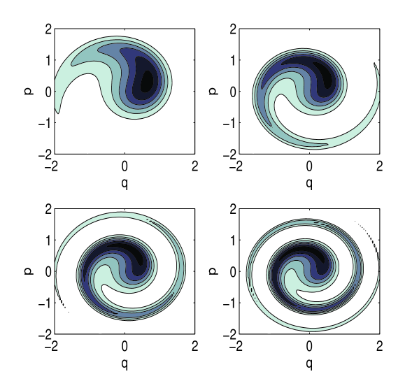
Figure 1: (Color online) Density plots showing the classical evolution of an initial Gaussian density centered at $\alpha_{0}=q_{0}=0.5$, with $\kappa=2$, as generated by the Hamiltonian $H=H_{0}^{2}/E$. The parameters $m,\omega,E$ have been set equal to $1$, and the times of the plots are, from left to right and top to bottom, $t=\pi/4$, $t=\pi/2$, $t=3\pi/4$ and $t=\pi$.

We are interested in the statistical properties of the evolving classical state, such as the mean values of position and momentum and the variance in these quantities. In general these statistics must be determined numerically, but the calculations may be simplified for certain classes of Liouville densities. We consider Gaussian densities

$$\rho_{\gamma,(q_{0},p_{0})}(q,p)\,=\,\frac{\omega}{2\pi\gamma^{2}}\exp(-(\tfrac{1}{2}m\omega^{2}(q-q_{0})^{2}+\tfrac{1}{2}(p-p_{0})^{2}/m)/\gamma^{2})\,,$$

which can be rewritten as

$$\rho_{\kappa,\,\alpha_{0}}(\alpha)\,=\,\frac{\kappa}{2\pi}\exp(-\kappa|\alpha-\alpha_{0}|^{2})\,,$$ (19)

where $\kappa=\hbar\omega/\gamma^{2},\quad\alpha_{0}=(\sqrt{m\omega}q_{0}+ip_{0}/\sqrt{m\omega})/\sqrt{2\hbar}$, and the effect of the change of measure has been incorporated into the normalisation co-efficient.

When the initial density is of this form, the $m$th moment of $\alpha$ at time $t$ is given by

$$\langle\alpha^{m}\rangle(t)\,=\,\frac{\kappa}{\pi}\int_{\mathbb{C}}\alpha^{m}e^{-i\omega mtH^{\prime}(\hbar\omega\,\overline{\alpha}\alpha)}e^{-\kappa|\alpha-\alpha_{0}|^{2}}d^{2}\alpha\,.$$ (20)

This integral can be simplified by setting $\alpha=r\exp(i\phi)/\sqrt{2}$ and $\alpha_{0}=r_{0}\exp(i\phi_{0})/\sqrt{2}$ and then evaluating the integral over $\phi$ so that

$$\langle\alpha^{m}\rangle(t)\,=\,\frac{\kappa}{2^{m/2}}e^{im\phi_{0}-\kappa r_{0}^{2}/2}\int_{0}^{\infty}r^{m+1}\,e^{-\kappa r^{2}/2}\,I_{m}(\kappa rr_{0})e^{-im\omega tH^{\prime}(\hbar\omega r^{2}/2)}dr\,,$$ (21)

where $I_{m}$ denotes the modified Bessel function [18] of the first kind of order $m$. The classical moments of primary interest are the mean and standard deviation in position and momentum. These can be constructed from the moments in $\alpha$ and $\overline{\alpha}$ as

$$\langle q\rangle(t)\,=\,\sqrt{(2\hbar/m\omega)}\,{\rm Re}\{\langle\alpha\rangle(t)\}\,,\qquad\langle p\rangle(t)\,=\,\sqrt{2\hbar m\omega}\,{\rm Im}\{\langle\alpha\rangle(t)\}\,,$$

$$\qquad\qquad\Delta q(t)\,=\,\sqrt{\hbar(\langle|\alpha|^{2}\rangle-{\rm Re}\{\langle\alpha\rangle(t)^{2}\})/m\omega-\langle q\rangle(t)^{2}}\,,\qquad\qquad$$

$$\qquad\qquad\Delta p(t)\,=\,\sqrt{\hbar m\omega(\langle|\alpha|^{2}\rangle-{\rm Re}\{\langle\alpha\rangle(t)^{2}\})-\langle p\rangle(t)^{2}}\,.\qquad\qquad$$ (22)

Note that the moment $\langle|\alpha|^{2}\rangle(t)=|\alpha_{0}|^{2}+1/\kappa$ is a constant of the motion.

If $K>1$, then it follows from (21) that $\langle\alpha^{m}\rangle(t)\to 0$ as $t\to\infty$ for every $m>0$, by the Riemann-Lebesgue Lemma [19]. In particular, the mean position and momentum tend towards zero as time increases. This is in sharp contrast to what happens with the corresponding quantum evolution, where periodic behaviour occurs [16].

On phase space, the quantum dynamics is determined by the Moyal bracket expansion (11), from which comparisons can be made with the classical dynamics in the phase space setting. As already indicated, the transition from classical to quantum dynamics can be studied by successively adding on to the classical Poisson bracket evolution, higher order terms in that expansion [1], [4] until the full quantum dynamics is obtained. Note that for polynomial Hamiltonians such as (14), the series (11) terminates. This process then defines a terminating sequence of semiclassical approximations, starting with the classical evolution, and ending with the quantum one.

On the other hand, in order to define semiquantum approximations to classical dynamics, we represent both the quantum and classical dynamics on Hilbert space in terms of the Hamiltonian operator $\hat{H}$ which, given (14), takes the form

$$\hat{H}\,=\,\mathcal{W}^{-1}(H)\,=\,E\sum_{k=0}^{K}c_{k}\left(\hat{H}_{0}/E\right)^{k}\,.$$ (23)

The dimensionless co-efficients $c_{k}$ are determined by, but are not identical to, the $b_{k}$ in (14), except that $c_{K}=b_{K}$. For example if $H=H_{0}^{3}/E^{2}$, then $\hat{H}=\hat{H}_{0}^{3}/E^{2}+5(\hbar\omega)^{2}\hat{H}_{0}/4E^{2}$ as in(40) below. The relation between the coefficients $b_{k}$ and $c_{l}$ can be determined using recurrence relations, but explicit formulas are very complicated. What is important to note here is that, with $H$ a ‘classical’ Hamiltonian and the $b_{k}$ assumed independent of $\hbar$, the $c_{k}$ for $k>0$ typically have the form $c_{k}=b_{k}+{\rm o}(\hbar)$ as $\hbar\to 0$.

Since ${\hat{H}}$ is a function of the oscillator Hamiltonian operator $\hat{H}_{0}$, it can be diagonalised on the well-known number eigenstates. We introduce the creation and annihilation operators $\hat{a}=\mathcal{W}^{-1}(\alpha)$ and $\hat{a}^{\dagger}=\mathcal{W}^{-1}(\overline{\alpha})$, and the number operator $\hat{N}=\hat{a}^{\dagger}\hat{a}$, so that $\hat{H}_{0}=\hbar\omega(\hat{N}+1/2)$. Then $\hat{H}$ is diagonal on the states $|n\rangle$, $n=0,\,1,\,2,\,\dots$ with $\hat{N}\,|n\rangle=n|n\rangle$, and has eigenvalues given by

$$\lambda_{n}\,=\,E\sum_{k=0}^{K}c_{k}\left(\frac{\hbar\omega(n+1/2)}{E}\right)^{k}\,=\,E\sum_{k=0}^{K}c_{k}\,\mu^{k}\,(n+1/2)^{k}\,.$$ (24)

Our object is to construct semiquantum approximations by using the expansion (7) and, beginning with the quantum dynamics, to successively add on higher order correction terms to this until the full classical dynamics is obtained. Because the series (7) also terminates for polynomial Hamiltonians, we get in this way a terminating sequence of semiquantum approximations, beginning with the quantum evolution, and ending with the classical one.

4 Example 1: Hamiltonian of degree 4

The first example that we consider has

$$H=H_{0}^{2}/E,\qquad\hat{H}=\hat{H}_{0}^{2}/E+(\hbar\omega)^{2}/4=\mu\hbar\omega(\hat{N}^{2}+\hat{N}+1/2)\,.$$ (25)

Since $H$ is quadratic in $H_{0}$, and hence quartic in $q$ and $p$, the dynamics is nonlinear. It is then to be expected that the classical and quantum evolutions produce comparable values and behaviours of the expectation values of observables for only a limited period of time, sometimes referred to as the break time [20]. This depends on $\hbar$ and the properties of the initial state. The numerical value attributed to the break time in a particular case is dependent on which criterion is used to determine differences between the quantum and classical dynamics, so it should be interpreted only as a guide to the time-scale over the which the evolutions produce similar values for observable quantities.

Differences between the classical and quantum evolutions are already apparent if we compare the classical picture in Fig.1, with the quantum evolution of the Wigner function on phase space in Fig.2, which starts with the same initial Gaussian density, and covers the same length of time. In the first place, the Wigner function immediately develops negative values on some regions, shown in white in Fig.2. Secondly, the quantum evolution is periodic, unlike the classical evolution, with period $2\pi/\mu\omega$ in this case. This can be seen more clearly from the formula (27) below for the matrix elements of the density operator, all of which have this period. Many studies in recent years have explored in detail such characteristic differences between quantum and classical dynamics, especially in the context of ’chaos’ ; see for example [21, 22].

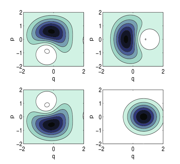
Figure 2: (Color online) Quantum evolution of an initial Gaussian Wigner function, with the same parameter values used in Figure 1, and shown at the same times. Regions on which the pseudo-density becomes negative are shown in white.

In this first example, the full classical evolution on Hilbert space is given by adding just the first correction to the quantum evolution in (7), and hence in this case there are only the zeroth order semiquantum dynamics and the full classical dynamics to study. Similarly, the full quantum evolution on phase space is given with just the first correction to the classical evolution in (11), so there are only zeroth order semiclassical dynamics and the full quantum dynamics to study. In short, there is no dynamics ‘in between’ the classical and quantum dynamics in this case. Nevertheless, the simplicity of this example makes it relatively easy to derive analytic expressions for the classical dynamics on Hilbert space that are relevant to more complicated cases.

The quantum evolution in Hilbert space $\mathcal{H}$ in this example is determined by

$$\frac{d\hat{\rho}}{dt}\,=\,\frac{(\hbar\omega)^{2}}{i\hbar E}[\hat{N}(\hat{N}+1),\hat{\rho}]=-i\mu\omega[\hat{N}(\hat{N}+1),\hat{\rho}]\,.$$ (26)

If we represent $\hat{\rho}$ in the number basis, its matrix elements $\rho_{nm}\,=\,\langle n|\hat{\rho}|m\rangle$ then evolve as

$$\rho_{nm}(t)\,=\,e^{-it(E_{n}-E_{m})/\hbar}\rho_{nm}(0)\,,$$ (27)

where $E_{n}$, $E_{m}$ are eigenvalues of $\hat{H}$ with, from (24), $E_{n}=\mu\hbar\omega(n^{2}+n+1/2)$.

Changing variables from $(q,p)$ to $(\alpha,\overline{\alpha})$, we find the classical evolution (7), on $\mathcal{H}$ in this example as

$$\frac{d\hat{G}}{dt}\,=\,-i\mu\,\omega\,[\hat{N}(\hat{N}+1),\hat{G}]\qquad\qquad$$

$$-\frac{1}{24i\hbar}\left([\hat{H}_{\alpha\alpha},\hat{G}_{{\overline{\alpha}}\overline{\alpha}}]-2[\hat{H}_{\alpha\overline{\alpha}},\hat{G}_{\alpha\overline{\alpha}}]+[\hat{H}_{\overline{\alpha}\overline{\alpha}},\hat{G}_{\alpha\alpha}]\right)\,,$$ (28)

where $\hat{H}_{\alpha\alpha}=\mathcal{W}^{-1}(\partial^{2}H/\partial\alpha^{2}),\,\hat{H}_{\alpha\overline{\alpha}}=\mathcal{W}^{-1}(\partial^{2}H/\partial\alpha\partial\overline{\alpha})$, etc. In this expression the correction term appears to be of lower order in $\hbar$ than the zeroth order term because we have introduced the operator $\hat{N}$ which is ${\rm O}(1/\hbar)$, and derivatives with respect to $\alpha$ and $\overline{\alpha}$ which are ${\rm O}(\sqrt{\hbar})$. After some algebraic manipulation, (28) simplifies to

$$\frac{d\hat{G}}{dt}\,=\,-i(\mu\omega/2)\left([\hat{N}(\hat{N}+1),\hat{G}]+[\hat{N},\hat{a}\hat{G}\hat{a}^{\dagger}+\hat{a}^{\dagger}\hat{G}\hat{a}]\right)\,.$$ (29)

Note that although as remarked above this must be fully equivalent to the classical evolution of the Liouville density, there is still dependence on $\hbar$ in the RHS, because of the dependence implicit in the definition of ${\hat{G}}$. The effect of the evolution (29) can be made clearer if we write $\hat{G}$ as the ‘operator vector’ $|G\rangle\rangle\in\mathcal{H}\otimes\mathcal{H}^{*}$ [8] and replace the right and left action of operators on $\hat{G}$ by superoperators [23, 24, 6] acting on $|G\rangle\rangle$, labelled by the subscripts $r$ and $l$ respectively, i.e. $\hat{A}_{l}|\hat{G}\rangle\rangle\equiv\hat{A}\hat{G}$ and $\hat{A}_{r}|\hat{G}\rangle\rangle\equiv\hat{G}\hat{A}^{\dagger}$. We can then rewrite (29) in the operator vector form

$$\frac{d|G\rangle\rangle}{dt}\,=\,-i(\mu\omega/2)(\hat{N}_{l}-\hat{N}_{r})\left(\hat{N}_{l}+\hat{N}_{r}+1+\hat{a}_{l}\hat{a}_{r}+\hat{a}^{\dagger}_{l}\hat{a}^{\dagger}_{r}\right)|G\rangle\rangle\,.$$ (30)

If we now define the new superoperators

$$\hat{N}_{-}=\hat{N}_{l}-\hat{N}_{r}\,,\qquad\hat{X}_{1}=(\hat{N}_{l}+\hat{N}_{r}+1)/2\,,$$

$$\hat{X}_{2}=(\hat{a}_{l}\hat{a}_{r}+\hat{a}^{\dagger}_{l}\hat{a}^{\dagger}_{r})/2\,,\qquad\hat{X}_{3}=(\hat{a}_{l}\hat{a}_{r}-\hat{a}^{\dagger}_{l}\hat{a}^{\dagger}_{r})/2\,,$$ (31)

then the $\hat{X}_{i}$ close to form an $sl(2)$ algebra of superoperators that commute with $\hat{N}_{-}$ and satisfy on $\mathcal{H}\otimes\mathcal{H}^{*}$ the commutation relations

$$[\hat{X}_{2},\hat{X}_{1}]=\hat{X}_{3}\,,\quad[\hat{X}_{3},\hat{X}_{2}]=\hat{X}_{1}\,,\quad[\hat{X}_{3},\hat{X}_{1}]=\hat{X}_{2}\,.$$ (32)

In terms of these new superoperators, the classical evolution of $|G\rangle\rangle$ is given by

$$d|G\rangle\rangle\,/dt\,=\,-i\mu\,\omega\,\hat{N}_{-}(\hat{X}_{1}+\hat{X}_{2})|G\rangle\rangle\,.$$ (33)

Since the $sl(2)$ superoperators commute with $\hat{N}_{-}\,$, one method of simplifying the evolution is to decompose the tensor product space $\mathcal{H}\otimes\mathcal{H}^{*}$ into representations of $sl(2)$ labelled by the eigenvalues of $\hat{N}_{-}\,$. These eigenvalues may take any integer value $\nu\in\mathbb{Z}$ and the corresponding $sl(2)$ lowest-weight operator eigenvector of ${\hat{X}}_{1}$ is given by $|\nu,0\rangle\rangle$ for $\nu\geq 0$ and $|0,-\nu\rangle\rangle$ for $\nu<0$. Here we have introduced the basis of operator vectors $\{|n,m\rangle\rangle,\,n,m=0,1,2,\ldots\}$ in $\mathcal{H}\otimes\mathcal{H}^{*}$, that corresponds to the basis of operators $\{|n\rangle\langle m|,\,n,m=0,1,2,\ldots\}$ in the space of operators acting on $\mathcal{H}$, with $\hat{N}_{l}|n,m\rangle\rangle=n|n,m\rangle\rangle$ and $\hat{N}_{r}|n,m\rangle\rangle=m|n,m\rangle\rangle$.

Now we can write

$$|G\rangle\rangle=\sum_{\nu\in\mathbb{Z}}\,|G^{(\nu)}\rangle\rangle\,,$$ (34)

where

$$|G^{(\nu)}\rangle\rangle=\left\{\begin{array}[]{r@{\quad}l}\sum_{n=0}^{\infty}G_{n}^{(\nu)}|n+\nu,n\rangle\rangle&,\quad\nu\geq 0\\ \\ \sum_{n=0}^{\infty}G_{n}^{(\nu)}|n,n-\nu\rangle\rangle&,\quad\nu<0\end{array}\right.$$ (35)

with

$$G_{n}^{(\nu)}=\langle\langle n+\nu,n|G\rangle\rangle=\langle n+\nu|\hat{G}|n\rangle\quad{\rm for}\quad\nu\geq 0\,,$$

$$G_{n}^{(\nu)}=\langle\langle n,n-\nu|G\rangle\rangle=\langle n|\hat{G}|n-\nu\rangle\quad{\rm for}\quad\nu<0\,.$$ (36)

The classical evolution (33) of $|G\rangle\rangle$ generated by $\hat{H}$ now leads to

$$|G(t)\rangle\rangle\,=\,\sum_{\nu\in\mathbb{Z}}|G^{\nu}(t)\rangle\rangle\,=\,\sum_{\nu\in\mathbb{Z}}\exp(-i\nu\mu\omega\,t\hat{P}^{(\nu)})|G^{(\nu)}(0)\rangle\rangle\,,$$ (37)

where the only nonzero matrix elements of the superoperator $\hat{P}^{(\nu)}$ are given by

$$(\hat{P}^{(\nu)})_{nn}\,=\,n+(|\nu|+1)/2\,,\,\qquad\qquad\qquad\qquad$$

$$(\hat{P}^{(\nu)})_{nn+1}\,=\,(\hat{P}^{(\nu)})_{n+1n}\,=\,\sqrt{(n+1)(n+|\nu|+1)}\,/2\,.$$ (38)

As a counterpoint to the quantum evolution (27) of the matrix elements of $\hat{\rho}$, we find that the classical evolution transforms the matrix elements of $\hat{G}$ along each diagonal independently:

$$G_{nm}(t)\,=\,\sum_{r=0}^{\infty}\left(\exp[-i(n-m)\mu\omega t\hat{P}^{(n-m)}]\right)_{mr}\,G_{n-m+r\,r}(0)\,,$$ (39)

for $n\geq m$. By the $\nu$th diagonal, we mean the set of matrix elements for which the row label minus the column label is equal to $\nu$. If $\hat{G}$ is initially Hermitian, then it remains Hermitian under this evolution and the matrix elements of $\hat{G}(t)$ above the main diagonal can be obtained by complex conjugation from those below.

We can deduce at once several properties of the classically evolved matrix $\hat{G}(t)$ by recalling some properties of the classical evolution on the phase plane. Firstly, the total amount of probability on the plane remains constant, which implies that the trace of $\hat{G}(t)$ should also remain constant. That this is reproduced in the Hilbert space analysis can be seen from (39) by setting $n=m$ and observing that the diagonal elements of $\hat{G}$ are constants of the motion. Secondly, the integral over phase space of the square of the Liouville density is also a constant of the motion, and this is equivalent to the Hilbert space condition that $\textrm{Tr}(\hat{G}(t)^{2})$ should remain constant. This property of $\hat{G}(t)$ can be verified from (39) by noting that the evolution of each diagonal of $\hat{G}(t)$ is unitary and hence that the sum of the squares of the elements of the $\nu$th diagonal is a constant of the motion. It then follows that the sum over all diagonals, equal to $\textrm{Tr}(\hat{G}(t)^{2})$, is also a constant.

Note however that the classical evolution generated by $\hat{H}$ is not unitary in the sense one uses when describing quantum dynamics, that is to say, in the Hilbert space $\mathcal{H}$. Instead, it defines an evolution of $\hat{G}$ that corresponds to a unitary superoperator evolution of the operator vector $|\rho\rangle\rangle$ in $\mathcal{H}\otimes\mathcal{H}^{*}$. This has the consequence that some features of a quantum evolution remain, such as the trace relations described above, but that other characteristic features of a quantum evolution are lost. For example, there is no requirement for the eigenvalues of the Groenewold operator to remain constant under the motion. These eigenvalues can and do change and in general, negative eigenvalues will typically develop over time, even if all eigenvalues of $\hat{G}$ are intially non-negative.

When examining the relationship between quantum and classical dynamics, it is primarily of interest to consider the limit $\hbar\rightarrow 0$ in some appropriate way. There is some flexibility in how to do this. In [16], the limit was taken in such a way that the initial phase space density approaches a delta-function in $q$ and $p\,$, so that both the quantum and classical dynamics approach that of a classical trajectory. In this paper, we shall instead investigate numerically the effect of reducing the value of $\hbar$ in such a way that the initial Gaussian phase space density is kept unchanged.

This involves a scaling of three key parameters: $\kappa$, $\mu$ and $\alpha_{0}$. The first two of these depend linearly on $\hbar$, while $\alpha_{0}$ is linear in $(1/\sqrt{\hbar})$. In order to keep the initial density constant as $\hbar\rightarrow 0$, we must have $\kappa$, $\mu\rightarrow 0$ and $\alpha_{0}\rightarrow\infty$, while keeping $\kappa/\mu$ and $\kappa|\alpha_{0}|^{2}$ constant.

In Fig.3, we graph the first and second moments of $\alpha$ for two sets of the parameters $\kappa$, $\mu$ and $\alpha_{0}$, with $t$ in the range $[0,\pi]$. For the top two graphs in Fig.3, the values $\kappa=2$, $\mu=1/2$ and $\alpha_{0}=1/2$ are used, while in the bottom two graphs, the values $\kappa=1,\mu=1/4$ and $\alpha_{0}=1/\sqrt{(}2)$ are used, corresponding to $\hbar\rightarrow\hbar/2$. The first moments are graphed on the left in Fig.3, and it can be seen that the quantum evolution lies close to the classical for much longer with the smaller (effective) value of $\hbar$. A more exaggerated sign of this convergence can be seen in the graphs of the second moments on the right. In the upper graph, one can see that the classical moment approaches the origin, whereas the quantum moment exhibits a symmetry in $q$. This symmetry is a sign of the recurrence of the initial state at $t=2\pi$. In the lower graph however, the recurrence is not due to occur until $t=4\pi$ and the quantum evolution resembles the classical much more closely for $t\in[0,2\pi]$.

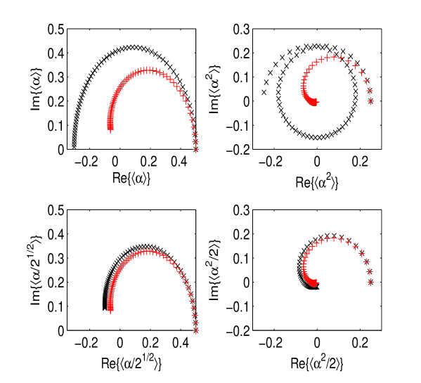
Figure 3: (Color online) Classical and quantum evolution of the first and second moments of $\alpha=(q+ip)/\sqrt{2}$ as generated by $H=H_{0}^{2}/E$. Points on the classical curves are marked by + and points on the quantum curves by x. Again $m=\omega=E=1$, and here $q_{0}=\sqrt{2},p_{0}=0$. The first moments are graphed on the left and the second moments on the right. In the two upper graphs, $\kappa=2,\mu=1/2,\alpha_{0}=1/2$ and in the lower two graphs, $\kappa=1,\mu=1/4,\alpha_{0}=1/\sqrt{(}2)$.

5 Example 2: Hamiltonian of degree 6

In order to compare and contrast semiquantum and semiclassical dynamics, we need to select a Hamiltonian of least degree 3 in $H_{0}$, so that there are nontrivial semiclassical and semiquantum approximations lying between classical and quantum dynamics. The simplest such case has

$$H=H_{0}^{3}/E^{2}\,,\quad\hat{H} = \hat{H}_{0}^{3}/E^{2}+5(\hbar\omega)^{2}\hat{H}_{0}/4E^{2}$$ (40)

$$= \mu^{2}\,\hbar\,\omega\,(\hat{N}^{3}+3\hat{N}^{2}/2+2\hat{N}+3/4)\,.$$

The eigenstates of $\hat{H}$ are again the number states and it is natural to represent the dynamical evolution in Hilbert space in this basis. The quantum evolution of the matrix elements of an initial density operator $\hat{\rho}(0)$ on $\mathcal{H}$ is again given by (27), where in this case the energy eigenvalues take the form $E_{n}=\mu^{2}\hbar\omega(n^{3}+3n^{2}/2+2n+3/4)$. From this we see that the quantum evolution is again periodic, but now with period $4\pi/\mu^{2}\omega$.

The equations governing the classical evolution of the Groenewold operator on $\mathcal{H}$ are obtained as before by inserting the Hamiltonian into equation (7). The result is that we obtain an expression for the full classical evolution that starts with the quantum evolution and adds two correction terms:

$$\frac{d\hat{G}}{dt}=-i\mu^{2}\hbar\omega\left[\hat{N}^{3}+3\hat{N}^{2}/2+2\hat{N},\hat{G}\right]\qquad\qquad\quad$$

$$-\frac{1}{24i\hbar}\left([\hat{H}_{\alpha\alpha},\hat{G}_{{\overline{\alpha}}\overline{\alpha}}]-2[\hat{H}_{\alpha\overline{\alpha}},\hat{G}_{\alpha\overline{\alpha}}]+[\hat{H}_{\overline{\alpha}\overline{\alpha}},\hat{G}_{\alpha\alpha}]\right)\qquad\qquad$$

$$+\frac{7}{5760i\hbar}\left(-4[\hat{H}_{\alpha\alpha\alpha\overline{\alpha}},\hat{\rho}_{{\alpha\overline{\alpha}}\overline{\alpha}\overline{\alpha}}]+6[\hat{H}_{{\alpha\alpha\overline{\alpha}}\overline{\alpha}},\hat{G}_{{\alpha\alpha\overline{\alpha}}\overline{\alpha}}]-4[\hat{H}_{\alpha\overline{\alpha}\overline{\alpha}\overline{\alpha}},\hat{G}_{{\alpha\alpha\alpha\overline{\alpha}}}]\right)\,.$$ (41)

Note that terms involving fourth derivatives with respect to $\alpha$ and $\overline{\alpha}$ do not appear in the second classical correction, because $\partial^{4}H/\partial\alpha^{4}$ and $\partial^{4}H/\partial\overline{\alpha}^{4}$ vanish in this example.

The correction terms can be simplified by straightforward but lengthy algebraic manipulation. Of particular interest is the semiquantum evolution equation that includes the quantum evolution and the first classical correction. This equation simplifies to

$$\frac{d\hat{G}}{dt}=-i(\mu^{2}\,\hbar\,\omega/4)\left(5[\hat{N}^{2},\hat{a}^{\dagger}\hat{G}\hat{a}]+5[\hat{N}(\hat{N}+2),\hat{a}\hat{G}\hat{a}^{\dagger}]\right.$$

$$\left.-[\hat{N}(\hat{N}+1)(\hat{N}+2),\hat{\rho}]-[\hat{N},\hat{a}^{2}\hat{\rho}\hat{a}^{\dagger 2}+\hat{a}^{\dagger 2}\hat{\rho}\hat{a}^{2}+3\hat{N}\hat{\rho}\hat{N}]\right)\,.$$ (42)

If we make use of the $sl(2)$ operators (31) introduced earlier, then the corresponding evolution equation for the operator vector $|G\rangle\rangle$ is given in this case by

$$d|G\rangle\rangle/dt\,=\,-i\mu^{2}\omega\hat{N}_{-}\left(3(\hat{X}_{1}\hat{X}_{2}+\hat{X}_{2}\hat{X}_{1})/2-(\hat{X}_{1}-\hat{X}_{2})^{2}\right)|G\rangle\rangle\,.$$ (43)

The solution of this equation has similar properties to the solution of (33). In particular, it can again be decomposed as in (34), leading in this case to an expression of the form

$$|G(t)\rangle\rangle\,=\,\sum_{\nu\in\mathbb{Z}}|G^{\nu}(t)\rangle\rangle\,=\,\sum_{\nu\in\mathbb{Z}}\exp(-i\nu\mu^{2}\omega t\hat{Q}^{(\nu)})|G^{\nu}(0)\rangle\rangle$$ (44)

in place of (37). However in this case, truncation methods for determining the eigenvalues of $\hat{Q}^{\nu}$ appear to fail, and hence for computational purposes, it is useful first to introduce the unitary $sl(2)$ operator $\hat{U}=\exp(\log(7/3)\hat{X}_{3}/4)$ which enables us to simplify the expression in (43), as

$$\hat{U}\,\left(3(\hat{X}_{1}\hat{X}_{2}+\hat{X}_{2}\hat{X}_{1})/2-(\hat{X}_{1}-\hat{X}_{2})^{2}\right)\,\hat{U}^{\dagger}=\sqrt{21}\,\left(\hat{X}_{1}\hat{X}_{2}+\hat{X}_{2}\hat{X}_{1}\right)\,.$$ (45)

This is seen after noting from (31) and (32) that

$$3(\hat{X}_{1}\hat{X}_{2}+\hat{X}_{2}\hat{X}_{1})/2-(\hat{X}_{1}-\hat{X}_{2})^{2} = 3{\hat{X}}_{+}^{2}/4-7{\hat{X}}_{-}^{2}/4\,,$$

$${\hat{X}}_{1}{\hat{X}}_{2}+{\hat{X}}_{2}{\hat{X}}_{1} = ({\hat{X}}_{+}^{2}-{\hat{X}}_{-}^{2})/4\,,$$ (46)

where

$${\hat{X}}_{\pm}={\hat{X}}_{2}\pm{\hat{X}}_{1}\,,\qquad{\hat{X}}_{3}\,{\hat{X}}_{\pm}={\hat{X}}_{\pm}({\hat{X}}_{3}\pm 1)\,.$$ (47)

The transformation (45) maps $\hat{Q}^{(\nu)}$ to a tri-diagonal matrix $\hat{Q}^{(\nu)^{\prime}}$, whose only non-zero matrix elements are given by

$$\hat{Q}^{(\nu)^{\prime}}_{n+1\,n}\,=\,\hat{Q}^{(\nu)^{\prime}}_{n\,n+1}\,=\,\sqrt{21}(n+1+|\nu|/2)\sqrt{(n+1)(n+|\nu|+1)/2}\,,$$ (48)

and for which the eigenvalues can easily be determined numerically. The expression for the individual matrix elements of the Groenewold operator in this semiquantum approximation is now given by

$$G_{nm}(t)\,=\,\sum_{r,s,t=0}^{\infty}U^{(n-m)}_{mr}\exp\left(-i(n-m)\mu^{2}\omega t\hat{Q}^{(n-m)^{\prime}}\right)_{rs}U^{(n-m)\dagger}_{st}G_{n-m+t,t}(0)\,,$$ (49)

where $U^{(\nu)}_{nm}=\langle n+\nu,n|\hat{U}|m+\nu,m\rangle$ for $\nu\geq 0$.

In order to determine the full classical evolution on Hilbert space, we need to evaluate both correction terms in (41). This leads in place of (33) to a comparatively simple expression for the evolution of the operator vector $|G\rangle\rangle$:

$$\frac{d|G\rangle\rangle}{dt}\,=\,-3i\omega\mu^{2}/4\hat{N}_{-}(\hat{X}_{1}+\hat{X}_{2})^{2}|G\rangle\rangle\,.$$ (50)

Note that this evolution again depends on the operator sum $\hat{X}_{1}+\hat{X}_{2}$. This property turns out to be shared by the classical evolution for each Hamiltonian of the form (14). The formula corresponding to (50) in the general case is

$$\frac{d|G\rangle\rangle}{dt}\,=\,-i\omega\hat{N}_{-}\sum_{k=0}^{N}\frac{(k+1)c_{k}\mu^{k}}{2^{k}}(\hat{X}_{1}+\hat{X}_{2})^{k}|G\rangle\rangle\,.$$ (51)

However, expressions for the successive semiquantum approximations to the quantum evolution, such as (43), are not so easy to obtain for a general Hamiltonian of the form (14).

Returning to the example at hand, with ${\hat{H}}$ as in (40), the classical evolution of the matrix elements of $\hat{G}$ is given by

$$G_{nm}(t)\,=\,\sum_{r=0}^{\infty}\left(\exp[-i(n-m)\mu^{2}\omega t\left({\hat{P}}^{(n-m)}\right)^{2}]\right)_{mr}G_{n-m+r,r}(0)\,,$$ (52)

with ${\hat{P}}^{(\nu)}$ as in (38). Eqn. (52) is to be compared with (39) in the previous section. Working from (49) and (52), we can evaluate and compare various quantities of interest in the semiquantum and classical evolutions, such as the expectaton values of $\alpha$, and the eigenvalues of the Groenewold operator.

There is also a semiclassical approximation to be studied in this case. The classical dynamics involves two correction terms to the quantum evolution, and the quantum dynamics involves two correction terms to the classical evolution. Just as the semiquantum dynamics includes the first correction to the quantum dynamics but not the second, so the semiclassical dynamics includes the first correction to the classical dynamics but not the second. It is of particular interest to determine differences between the semiquantum and the semiclassical dynamics.

In Fig.(4), we show phase space plots of the evolution of the expectation value of $\alpha$ in the semiclassical and semiquantum approximations, along with the classical and quantum evolutions. The parameter values were chosen to be $\kappa=2$, $\mu=1/2$ and $\alpha_{0}=1/2$, and the time evolution is over the interval $[0,\pi]$. It is immediately clear that the semiclassical and semiquantum approximations are quite distinct. For small values of $t$, they closely approximate the quantum and classical moments respectively. However, the long-term behaviour is very different, as the semiquantum moment begins to oscillate in a fashion that is qualitatively similar to the quantum moment, whereas the semiclassical moment appears to approach smoothly a fixed constant, just as is the case for the classical moment.

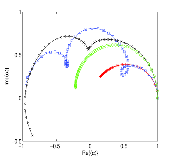
Figure 4: (Color online) Comparison of first moments of $\alpha=(q+ip)/\sqrt{2}$ for classical, semiquantum, quantum and semiclassical evolutions generated by the Hamiltonian $H=H_{0}^{3}/E^{2}$. Points on the classical, quantum, semiclassical and semiquantum curves are labelled by +, x, o and $\square$, respectively. The evolution is over the time-interval $[0,\pi]$ and again $m=\omega=E=1$, with $\kappa=2,\mu=1/2,\alpha_{0}=0.5$.

How does the behaviour change as $\hbar$ decreases? To examine this, we graph in Fig.(5) the first moment in $\alpha$ over $t\in[0,\pi]$, but this time with the parameter choices $\kappa=1,\mu=1/4,\alpha_{0}=1/\sqrt{2}$, which is equivalent to dividing $\hbar$ by two. The first thing one observes is that the quantum evolution is now much closer to the classical, although it begins to oscillate near $t=\pi$. It is also apparent that the semiquantum and semiclassical curves are good approximations to the classical and quantum moments respectively over most of the time-interval. One can also add that the semiclassical moment appears to be a good approximation to the quantum moment for a longer time than the semiquantum moment is a good approximation to the classical moment.

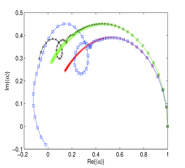
Figure 5: (Color online) Identical to the preceding Figure except that $\hbar$ has been reduced by a factor of two, by setting $\kappa=1,\mu=1/4,\alpha_{0}=1/\sqrt{2}$.

All the forms of dynamics can be studied in phase space or in Hilbert space. However, it must be emphasized that here as in general, the zeroth order semiclassical approximation to quantum dynamics, namely classical dynamics itself, when applied in Hilbert space with an initial Groenewold operator ${\hat{G}}(0)$ that is the image ${\cal W}^{-1}(2\pi\hbar\rho)$ of an initial Liouvillean density, will in general produce a ${\hat{G}}(t)$ that is not positive-definite for times $t>0$, even if ${\hat{G}}(0)$ is positive-definite, which it need not be. Closely related observations have been made in earlier studies of the evolution of density operators under classical dynamics [8, 23, 24, 25].

Conversely, the zeroth order semiquantum dynamics, namely quantum dynamics itself, when applied with an initial Wigner function $W(q,\,p,\,0)$ that is the image ${\cal W}({\hat{\rho}}/2\pi\hbar)$ of an initial quantum density operator, will in general produce a $W(q\,,p\,,t)$ that is not positive-definite for times $t>0$, even if $W(q,\,p,\,0)$ is positive-definite, which it need not be.

The preceding figures use measures of comparison that are natural in the phase space formulation of all the dynamics. Alternatively, one can use measures that are typically associated with formulations on Hilbert space. In particular, one can examine the evolution of the eigenvalues of the density operator (or the Groenewold operator) in the classical, quantum, semiclassical and semiquantum approximations. In Fig.(6) we show the evolution of the largest pair and smallest pair of eigenvalues for the classical, semiquantum and semiclassical cases. In the quantum case, the eigenvalues are $0$ and $1$ at all times as the system is in a pure (coherent) state initially, and stays in a pure state at all subsequent times. The parameter choices and time interval used in Fig.(6) correspond to those used in Fig.(4). We also single out the points at which $t=1,2,3$ on each graph for the purpose of comparison with the moment curve of Fig.(4) which is reproduced in Fig.(6). From these graphs, we observe that the semiquantum approximation to the classical moment is reasonable up till about $t=1$, by which time the eigenvalues of the classical and semiquantum Groenewold operators differ to a significant degree. The semiquantum eigenvalues appear to display periodic behaviour.

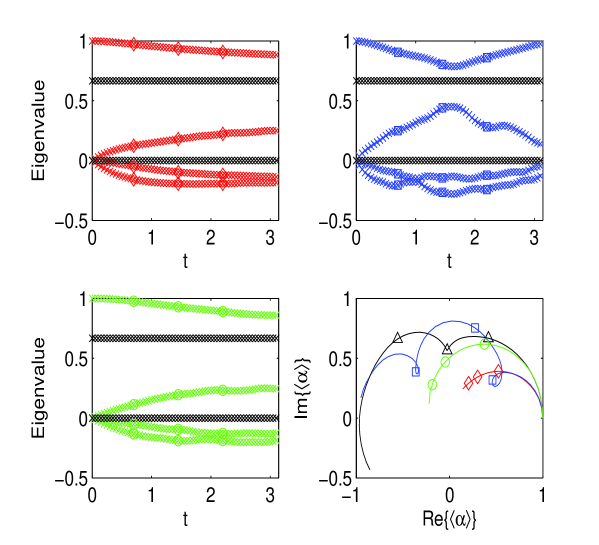
Figure 6: (Color online) Comparison of largest two and least two eigenvalues for, from left to right and top to bottom, classical, semiquantum and semiclassical evolutions generated by $H=H_{0}^{3}/E^{2}$, for the time interval $[0,\pi]$, and with $m=\omega=E=1$ and $\kappa=2,\mu=1/2,\alpha_{0}=0.5$. The evolution of the first moment is reproduced from Fig.5 in the graph at bottom right for comparison. Each of the other graphs also features the quantum spectrum $\{0,1\}$ and in all graphs the values at the time-points $t=1,2,3$ are marked $\lozenge$ (classical), o (semiclassical), $\triangle$ (quantum) and $\square$ (semiquantum).

The semiclassical eigenvalues remain very close to the classical eigenvalues over the whole time range. Since the behaviour of the individual eigenvalues does not seem to reflect the differences shown in the graphs of the first moment, this leads one to wonder if those differences are reflected in some global property of the spectrum. We know that in each case, the evolved Groenewold operators have trace and square trace equal to 1, but we can look at the contribution to these quantities by the negative eigenvalues. Numerical experiments indicate that it is difficult to calculate the sum of the negative eigenvalues by using truncation techniques, so we instead concentrate on the sum of the squares of the negative eigenvalues. In Fig.(7) we graph this ‘squared negativity’ for the parameter values used in Fig.(4)

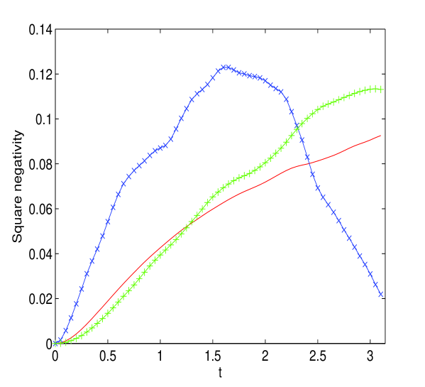
Figure 7: (Color online) Comparison of ‘square-negativity’ for classical, semi-quantum and semi-classical evolutions generated by $H=H_{0}^{3}/E^{2}$ for the time-interval $[0,\pi]$, and with $m=\omega=E=1$ and $\kappa=2,\mu=1/2,\alpha_{0}=0.5$. The solid line, the solid line with x points and the solid line with + points represent the classical, semiquantum and semiclassical values respectively.

These results, however, merely confirm the conclusions drawn from the eigenvalue curves and indicate that the spectrum of the semiclassical Groenewold operator resembles that of the classical Groenewold operator more closely than the spectrum of the semiquantum Groenewold operator does, for all but very small times. We conclude that the moments and the eigenvalue spectra provide quite different information about these different approximate dynamics.

6 Concluding remarks

Our study indicates that semiquantum approximations to classical dynamics can provide new information about the interface between quantum and classical mechanics. Semiquantum approximations obtained from the Hilbert space formulation of classical mechanics, and semiclassical ones obtained from the phase space formulation of quantum mechanics, show significantly different behaviours for expectation values of observables and eigenvalues of the (pseudo)density operator. For the simple systems considered here, it appears that a first semiquantum approximation to quantum dynamics is, for simple indicators like moments of coordinates and momenta, closer to classical dynamics and further from quantum dynamics than is a first semiclassical approximation to classical dynamics. On the other hand, as regards the spectrum of the density operator and Groenewold operator, the first semiclassical approximation behaves more like classical dynamics than the first semiquantum approximation, which behaves more like quantum dynamics in this respect. It is not at all clear why this should be so, and it is desirable in future work to look at cases where higher approximations come into play to see what happens then, as well as to examine the underlying theory more closely.

We have been able to consider only very simple one-dimensional systems here, and there is obviously a need also to explore systems with more degrees of freedom, especially nonintegrable ones. The possible role of semiquantum mechanics in throwing new light on the interface between classical chaos and corresponding quantum dynamics is especially interesting.

More generally, there are deep theoretical questions that arise about the mathematical relationship between semiquantum and semiclassical approximations, associated with the structure of the series expansions (7) and (11). Another concerns the nature of the relationship between action principles and semiquantum approximations to classical dynamics, whether formulated in phase space or Hilbert space. We hope to return to some of those questions.

Acknowledgement: We thank a referee for several useful comments and for bringing the papers of Vercin [6] and Voros [3] to our attention. This work was supported by Australian Research Council Grant DP0450778.

References

- [1] Wigner, E.P., Phys. Rev. 40, 749 (1932).
- [2] Maslov, V.P. and Fedoriuk, M.V., Semiclassical Approximation in Quantum Mechanics (Dordrecht, Reidel, 1981).
- [3] Voros, A., Phys. Rev. A 40, 6814 (1989).
- [4] Osborn, T. and Molzahn, F., Ann. Phys. 241, 79 (1995).
- [5] Bracken, A.J., J. Phys. A: Math. Gen. 36, L329 (2003).
- [6] Vercin, A. Int. J. Theoret. Phys. 39, 2063 (2000).
- [7] Groenewold, H., Physica 12, 405 (1946).
- [8] Muga, J.G. and Snider, R.F., Europhys. Lett. 19 (1992), 569–573.
- [9] Bracken, A.J. and Wood, J.G., Europhys. Lett. 68, 1–7 (2004).
- [10] Dubin, D.A., Hennings, M.A. and Smith, T.B., Mathematical Aspects of Weyl Quantization and Phase (Singapore, World Scientific, 2000).
- [11] Zachos, C., Int. J. Mod. Phys. 17, 297–316 (2002).
- [12] Bracken, A.J., Cassinelli, G. and Wood, J.G., J. Phys. A: Math. Gen. 36, 1033–1056 (2003).
- [13] Moyal, J., Proc. Camb. Phil. Soc. 45, 99 (1949).
- [14] Greiner, M., Mandel, O., Hansch, T.W. and Bloch, I., Nature 419, 51–54 (2002).
- [15] Dowling, M.R., Drummond, P.D., Davis, M.J. and Deuar, P., Phys. Rev. Lett. 94, 130401 (2005).
- [16] Milburn, G.J., Phys. Rev. A 33, 674 (1986).
- [17] Balescu, R., Equilibrium and Nonequilibrium Statistical Mechanics (New York, Wiley, 1975).
- [18] Abramowitz, M. and Stegun, I.A., Handbook of Mathematical Functions (New York, Dover, 1972).
- [19] Churchill, R.V., Fourier Series and Boundary Value Problems (New York, McGraw-Hill, 1963).
- [20] Emerson, J. and Ballentine, L.E., Phys. Rev. A 63, 052103 (2001).
- [21] Berry, M.V., Phil. Trans. R. Soc. A 287, 237 (1977).
- [22] Gutzwiller, M.C., Chaos in Classical and Quantum mechanics (New York, Springer-Verlag, 1990).
- [23] Muga, J.G., Sala, R. and Snider, R.F., Physica Scripta 47, 732 (1993).
- [24] Sala, R. and Muga, J.G., Phys. Lett. A 192 (1994), 180–184.
- [25] Habib, S., Jacobs, K., Mabuchi, H., Ryne, R., Shizume, K. and Sundaram, B., Phys. Rev. Lett. 88, 040402 (2002).