Optimal error tracking via quantum coding and continuous syndrome measurement

Abstract

We revisit a scenario of continuous quantum error detection proposed by Ahn, Doherty and Landahl [Phys. Rev. A 65, 042301 (2002)] and construct optimal filters for tracking accumulative errors. These filters turn out to be of a canonical form from hybrid control theory; we numerically assess their performance for the bit-flip and five-qubit codes. We show that a tight upper bound on the stochastic decay of encoded fidelity can be computed from the measurement records. Our results provide an informative case study in decoherence suppression with finite-strength measurement.

Prospects for quantum computation have motivated the development of an extensive theory of quantum error prevention/correction (QEC) Aliferis et al. . Despite experimental demonstrations of some key methods Langer et al. (2005); Chiaverini et al. (2004); Knill et al. (2001), there remains a significant gap between the abstract algebraic theory of QEC and concrete physical models of real quantum systems. In particular, QEC is still mainly discussed in terms of instantaneous measurement and recovery operations rather than more realistic continuous-time dynamical models. Bridging this gap would enable us, e.g., to deduce limits on QEC performance from the finite speed of laboratory measurement and recovery operations. Appropriate continuous-time formulations of QEC would likewise facilitate deeper connections with control theory, which could in turn lead to the discovery of new quantum memory schemes.

Our aim in this article will be to pursue a rigorous approach to incorporating finite-strength measurement within the familiar conceptual setting of discrete quantum error correcting codes. At the same time, we will arrive at familiar equations from classical control theory that should be amenable to characterization via established methods of stochastic analysis. While the specific models we consider—continuous-time relaxations of stabilizer codes as introduced by Ahn, Doherty and Landahl Ahn et al. (2002)—are rather impractical from an experimental point of view, they do provide a canonical setting in which to demonstrate how essential ideas from quantum error correction can be reconciled with stochastic control theory. We regard this as an important step towards developing a general theory of optimal decoherence suppression with resource constraints on measurement and control.

We begin by considering a continuous-time relaxation of the bit-flip code Ahn et al. (2002). A logical qubit state $|\Psi\rangle=c_{0}|0\rangle+c_{1}|1\rangle$ is encoded in the joint state of three physical qubits as $|\Psi\rangle\mapsto c_{0}|000\rangle+c_{1}|111\rangle\equiv|\Psi_{E}\rangle$. The system is coupled to decay channels that can cause independent Markovian bit flips and also to probe channels that allow for continuous (finite-strength) syndrome measurement Sarovar et al. (2004). Following Ahn et al. (2002); Sarovar et al. (2004), we assume that the syndrome measurements are constructed by coupling two probe fields to the syndrome generators Gottesman (1997) $M_{1}=ZZI=\sigma_{z}\otimes\sigma_{z}\otimes\openone$ and $M_{2}=ZIZ=\sigma_{z}\otimes\openone\otimes\sigma_{z}$. The total system dynamics is then described by the quantum stochastic differential equation (e.g. Gardiner and Zoller (2004))

$$dU_{t}=\{\sqrt{\gamma}\,(X_{1}\,dB^{1{\dagger}}_{t}+X_{2}\,dB^{2{\dagger}}_{t}+X_{3}\,dB^{3{\dagger}}_{t}-\mbox{h.c.})+\\ \sqrt{\kappa}\,(M_{1}\,dA^{1{\dagger}}_{t}+M_{2}\,dA^{2{\dagger}}_{t}-\mbox{h.c.})-(\tfrac{3}{2}\gamma+\kappa)\,dt\}\,U_{t}$$ (1)

where $B^{i}_{t}$ are the bit-flip channels, $A^{i}_{t}$ are the probe channels and $X_{1}=XII=\sigma_{x}\otimes\openone\otimes\openone$, $X_{2}=IXI$ et cetera. The unitary evolution $U_{t}$ is a Schrödinger picture propagator for the entire system including the probe fields.

For homodyne-type detection of the two probe channels we obtain two observation processes $Y^{i}_{t}=U_{t}^{\dagger}(A^{i}_{t}+A^{i{\dagger}}_{t})U_{t}$ that can be written (via quantum Itô rules) as

$$dY^{i}_{t}=2\sqrt{\kappa}\,U_{t}^{\dagger}M_{i}U_{t}\,dt+dA^{i}_{t}+dA^{i{\dagger}}_{t}$$ (2)

(this is called the input-output picture in Gardiner and Zoller (2004)). Similarly, we could in principle attempt to observe the bit-flip events directly by performing direct detection of the corresponding decay channels $B_{t}^{i}$; this would give rise to additional (counting) observations $Z^{i}_{t}$ that are independent Poisson processes with rate $\gamma$ (see, e.g., Bouten and Van Handel (2005)). Although the $Z_{t}^{i}$ are generally assumed to be unobservable in QEC, we will exploit them below to obtain useful information on the statistics of the measurement currents $Y_{t}^{i}$.

Our goal is to detect and to correct bit-flip errors by making use of the probe currents $Y_{t}^{i}$, $i=1,2$. Hence we must understand how best to extract information about error events from the noisy observed signals. We begin by calculating the least mean-square estimator for our system Bouten and Van Handel (2005), in the form of a (random) three-qubit density matrix $\rho_{t}$ (the conditional state). For every system observable $A$, ${\rm Tr}[A\rho_{t}]$ is the function of the observation history that minimizes the estimation error $\langle(U_{t}^{\dagger}AU_{t}-{\rm Tr}[A\rho_{t}])^{2}\rangle$. If we observe only $Y^{i}_{t}$, then $\rho_{t}$ obeys the quantum filtering equation Bouten and Van Handel (2005)

$$d\rho_{t}=\sum_{k=1}^{3}\gamma\,\mathcal{T}[X_{k}]\rho_{t}\,dt+\sum_{i=1}^{2}\kappa\,\mathcal{T}[M_{i}]\rho_{t}\,dt\\ +\sum_{i=1}^{2}\sqrt{\kappa}\,\mathcal{H}[M_{i}]\rho_{t}\,(dY_{t}^{i}-2\sqrt{\kappa}\,{\rm Tr}[M_{i}\rho_{t}]\,dt)$$ (3)

where $\mathcal{T}[X]\rho=X\rho X^{\dagger}-\rho$ and $\mathcal{H}[X]\rho=X\rho+\rho X^{\dagger}-{\rm Tr}[(X+X^{\dagger})\rho]\rho$. This is equivalent to the stochastic master equation used in Ahn et al. (2002). If we were to additionally observe the bit flip channels $Z_{t}^{i}$, we could obtain an improved estimator $\tilde{\rho}_{t}$ that would obey a “jump-unraveled” version of Eq. (3) with $\gamma\mathcal{T}[X_{k}]\,dt$ replaced by $\mathcal{T}[X_{k}]\,dZ_{t}^{i}$. An important feature of these equations Bouten and Van Handel (2005) is that the so-called innovations processes $dW_{t}^{i}=dY_{t}^{i}-2\sqrt{\kappa}\,{\rm Tr}[M_{i}\rho_{t}]\,dt$ are independent and have the law of a Wiener process.

We can use the fact that the innovations are Wiener processes, in the absence of ‘real’ (physically generated) measurement signals $Y_{t}^{i}$, to generate the latter through Monte Carlo simulations. By driving Eq. (3) with random sample paths of a Wiener process, we can reconstruct observation processes $Y_{t}^{i}$ that sample the space of measurement records with the correct probability measure. The evolution of the filter variables in each simulation fairly represents what would have happened if physically generated measurement records $Y_{t}^{i}$ had actually been presented to the filter and it derived $W_{t}^{i}$ from them. Similarly, we can reconstruct $Y_{t}^{i}$ from the jump-unraveled version of Eq. (3) by driving it with Wiener processes $\tilde{W}_{t}^{i}$ and independent Poisson processes $Z_{t}^{i}$ with rate $\gamma$. The innovations theorem guarantees that both simulations will generate sample paths $Y_{t}^{i}$ with the same probability measure. We will invoke this property later.

In the usual setting of discrete quantum codes, an instantaneous measurement of $M_{1}$ and $M_{2}$ after a period of free evolution is used to determine the recovery operation (if any) that should be applied. If $(M_{1},M_{2})=(+1,+1)$ no correction is necessary; outcomes $(-1,+1)$ mean that $IXI$ should be applied; $(+1,-1)\Rightarrow IIX$ and $(-1,-1)\Rightarrow XII$. These outcomes are called the error syndromes. In the continuous setting we introduce the orthogonal projectors $\Pi_{0}\ldots\Pi_{3}$ onto the eigenspaces corresponding to each syndrome. The quantity $p^{m}_{t}={\rm Tr}[\Pi_{m}\rho_{t}]$ is then the conditional probability (given the noisy probe observations) that, had we actually measured $M_{1}$ and $M_{2}$, we would have obtained the syndrome corresponding to $\Pi_{m}$. Plugging $p^{m}_{t}$ into Eq. (3) we obtain the syndrome filter

$$dp_{t}=\Lambda^{T}p_{t}\,dt+\sum_{i=1}^{2}(H_{i}-h_{i}^{T}p_{t}\,\openone)p_{t}\,(dY_{t}^{i}-h_{i}^{T}p_{t}\,dt)$$ (4)

where $h_{i}^{m}/2\sqrt{\kappa}$ is the outcome of $M_{i}$ corresponding to the syndrome $\Pi_{m}$, $H_{i}=\mbox{diag}\,h_{i}$, and $\Lambda_{mn}=\gamma(1-4\delta_{mn})$. The $p_{t}^{i}$ form a closed set of equations, as the observations are uninformative on the logical state of the qubit and the coherences (if any) between the syndromes.

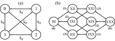
(c)

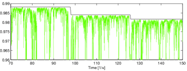
Figure 1: Markov chains associated to the three-qubit code: (a) the syndrome chain, and (b) the extended correction chain with the corresponding syndromes labeled between brackets. All transitions are independent with rate $\gamma$. (c) A Monte Carlo trajectory of $\max_{i}(p_{t}^{i})$ (green noisy curve) and $\mathfrak{J}_{t}$ (black step-like curve) for the five-qubit code with $\kappa/\Gamma=100$.

The syndrome filter, Eq. (4), is a familiar equation from classical probability theory; we will gain important insight by reducing our problem to a classical one. Consider a system that can be in one of four states labeled $0\ldots 3$. Suppose the system is in some known state at time $t$. After an infinitesimal time increment $dt$ the system can switch to one of the other three states, each of which occurs with probability $\gamma\,dt$. This defines a Markov jump process on a graph, as depicted in Fig. 1a. Unfortunately we cannot observe the state directly; instead, we are given two observation processes of the form $dY_{t}^{i}=h_{i}^{m_{t}}\,dt+dV_{t}^{i}$ where $V_{t}^{1,2}$ are two independent Wiener processes that corrupt our observations, and $m_{t}$ is the state of the Markov jump process at time $t$. As our observations are noisy we cannot know the system state with certainty at any time. However, we can calculate the conditional probability $p_{t}^{m}$ that it is in state $m$ at time $t$. This classical estimation problem is precisely solved by Eq. (4), known as the Wonham filter Wonham (1965); Elliott et al. (1995).

To help interpret this result, consider the jump-unraveled version of Eq. (3). In the same way that we obtained Eq. (4), we can substitute $\tilde{p}_{t}^{m}={\rm Tr}[\Pi_{m}\tilde{\rho}_{t}]$ and get a closed form expression. Assuming the initial state lies inside one of the syndrome spaces , it is readily verified that $[M_{1},\tilde{\rho}_{t}]=[M_{2},\tilde{\rho}_{t}]=0$ for all $t$ and we obtain

$$d\tilde{p}_{t}=\sum_{k=1}^{3}(\tilde{X}_{k}-\openone)\tilde{p}_{t}\,dZ_{t}^{k}$$ (5)

where $\tilde{p}_{0}$ is one of the unit vectors $e_{n}^{m}=\delta_{nm}$. Here $\tilde{X}_{1}$ is a matrix such that $\tilde{X}_{1}e_{0}=e_{1}$, $\tilde{X}_{1}e_{1}=e_{0}$, $\tilde{X}_{1}e_{2}=e_{3}$, and $\tilde{X}_{1}e_{3}=e_{2}$, and $X_{2,3}$ are defined similarly as shown in Fig. 1a. The solution of this equation is of the form $\tilde{p}_{t}=e_{m_{t}}$ where $m_{t}$ is the Markov jump process defined above. Since

$$d\tilde{W}_{t}^{i}=dY_{t}^{i}-h_{i}^{T}\tilde{p}_{t}\,dt=dY_{t}^{i}-h_{i}^{m_{t}}\,dt$$ (6)

must be a Wiener process that is independent from all $Z_{t}^{i}$, the statistics of the probe observations obtained from the quantum system are precisely described by the classical model of the previous paragraph. The Markov process $m_{i}$ is simply the error syndrome obtained by observing the bit flips directly, and the Wonham filter above has a natural classical interpretation as the best estimate of $m_{i}$ given only the noisy probe observations.

We now turn to the problem of error correction. Suppose that we let the system evolve for some time while propagating the filter Eq. (4) with the observations. At some time $T$ we pose the question: what operation, if any, should we perform on the system to maximize the probability of restoring the initial logical state $|\Psi_{E}\rangle$? We will assume that we can pulse the system sufficiently strongly (as compared to $\kappa,\gamma$) to perform essentially instantaneous bit flips on any of the physical qubits. The most obvious decision strategy simply mimics discrete error correction—given the most likely syndrome state $m_{*}=\mbox{arg\,max}_{m}\,p_{T}^{m}$, we do nothing if $m_{*}=0$ and otherwise we perform a bit flip on physical qubit $m_{*}$.

But it is possible to do better. Recall that the discrete error correction strategy is based on an assumption that at most one bit flip occurs in the interval $[0,T]$. This assumption may not hold in practice. With our continuous syndrome measurement, we do actually have some basis for estimating the total number (and kind) of bit flips that have occurred. Unfortunately this information does not reside in the statistic $p_{t}$, which only gives the conditional probabilities of the syndromes at the current time. We are seeking a non-Markovian decision policy that knows something about the history of the bit flips.

The classical machinery introduced above allows us to solve this problem optimally. To do this we simply extend the Markov jump process $m_{t}$ as shown in Fig. 1b. The states of the extended chain $\hat{m}_{t}$ are no longer the four syndromes but the eight error states that may obtain at any given time. Every syndrome corresponds to two error states, as is shown in Fig. 1b. We still consider the same observation processes, so error states that belong to the same syndrome give rise to identical observations. Thus on the basis of the observations, the two Markov chains are indistinguishable. Nonetheless the extended chain gives rise to a different estimator that provides precisely the information we want. As by construction the Wonham filter provides the optimal estimate, we conclude that the optimal solution to our problem is given by the Wonham filter for the extended chain, i.e., the eight-dimensional equation

$$d\hat{p}_{t}=\hat{\Lambda}^{T}\hat{p}_{t}\,dt+\sum_{i=1}^{2}(\hat{H}_{i}-\hat{h}_{i}^{T}\hat{p}_{t}\,\openone)\hat{p}_{t}\,(dY_{t}^{i}-\hat{h}_{i}^{T}\hat{p}_{t}\,dt)$$ (7)

where $\hat{\Lambda}$, $\hat{h}_{i}$ are the intensity matrix and observation vector for the chain $\hat{m}_{t}$ (see Wonham (1965); Elliott et al. (1995) for details). The optimal correction policy is now simple: at time $T$, we perform the correction that corresponds to the state $\hat{m}_{*}=\mbox{arg\,max}_{m}\,\hat{p}^{m}_{T}$. Hence if $\hat{m}_{*}=III$ we do nothing, if $\hat{m}_{*}=IXX$ we flip physical qubits 2 and 3, etc. This maximizes the probability of restoring $|\Psi_{E}\rangle$.

From Fig. 1b we can see how information is lost from the quantum memory. At time $t=0$ we begin in the no-error state $III$. A bit flip might occur which puts us, e.g., in the state $XII$, then $XIX$, etc. But as we are observing these changes in white noise there is always a chance that when two bit flips happen in rapid succession, we ascribe the corresponding observations to a fluctuation in the white noise background rather than to the occurrence of two bit flips. In essence, successive bit flips are resolvable only if they are separated by a sufficiently long interval that the filter can average away the white noise fluctuations (the signal-to-noise $4\kappa$ determines this timescale). Occasionally, multiple bit flips occur too rapidly and information is lost (e.g., $III\rightarrow XII\rightarrow XIX$ may be mistaken for $III\rightarrow IXI$ since the two final states have identical syndromes). It is evident from Fig. 1b that this rate of information loss is independent of the error state. Hence there is no point in applying corrective bit flips at intermediate times $t<T$, as this cannot slow the loss of information. As the Wonham filter is optimal by construction, we conclude that the correction policy described above is optimal .

How can we quantify the information loss from the system? By construction $\hat{p}_{t}^{*}=\max_{m}\hat{p}_{t}^{m}$ is the probability of correct recovery at time $t$. Unfortunately, as one can see in Fig. 1c, the quantity $\hat{p}_{t}^{*}$ fluctuates rather wildly in time. Thus it is not a good measure of the information content of the system, as it is very sensitive to the whims of the filter: the filter may respond to fluctuations in the measurement record by adjusting the state as if a bit flip had occurred, but then correct itself when it becomes evident that nothing happened. We actually want to find some quantity that gives a (sharp) upper bound on all future values of $\hat{p}_{t}^{*}$. This would truly measure the information content of the system, as it bounds the probability of correct recovery that can be achieved.

We claim that the quantity $\mathfrak{J}_{t}=\max_{m}(\hat{p}_{t}^{m}/(\hat{p}_{t}^{m}+\hat{p}_{t}^{\bar{m}}))$, which is a function of filter variables, provides a suitable measure of the information content at time $t$. Here $\bar{m}\neq m$ is the error state that corresponds to the same syndrome as $m$, so $\hat{p}_{t}^{m}+\hat{p}_{t}^{\bar{m}}=P_{t}^{m}$ is the probability of the syndrome corresponding to $m$. Hence we can interpret $\mathfrak{J}_{t}$ as the conditional probability of the error state $m$, given that the system is in the corresponding syndrome. Define $I_{t}^{m}=\hat{p}_{t}^{m}/(\hat{p}_{t}^{m}+\hat{p}_{t}^{\bar{m}})$ so that $\mathfrak{J}_{t}=\max_{m}I_{t}^{m}$. Direct application of the Itô rules gives

$$\frac{dI_{t}^{m}}{dt}=-\sum_{n\neq m}\hat{\Lambda}_{nm}\,\frac{P_{t}^{n}}{P_{t}^{m}}\,(I_{t}^{m}-I_{t}^{n}).$$ (8)

If we define $m_{t}^{*}=\mbox{arg\,max}_{m}\,I_{t}^{m}$, then we get

$$\frac{d\mathfrak{J}_{t}}{dt}=-\sum_{n\neq m_{t}^{*}}\hat{\Lambda}_{nm_{t}^{*}}\,\frac{P_{t}^{n}}{P_{t}^{m_{t}^{*}}}\,(\mathfrak{J}_{t}-I_{t}^{n})\leq 0.$$ (9)

Hence $\mathfrak{J}_{t}$ decreases monotonically, and moreover by construction we must have $\hat{p}_{t}^{m}\leq I_{t}^{m}$, so $\hat{p}_{t}^{*}\leq\mathfrak{J}_{t}\leq\mathfrak{J}_{s}$ for all $s<t$. Thus evidently $\mathfrak{J}_{t}$ bounds all future values of $\hat{p}_{t}^{*}$. One would expect the bound to be tight for sufficiently high signal-to-noise (as then $P_{t}^{m_{t}^{*}}$ will be close to one), which is indeed the case as can be seen in Fig. 1c.

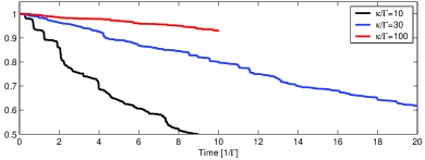
Figure 2: Average decay of $\mathfrak{J}_{t}$ for the five-qubit code (dependence on $\kappa/\Gamma$). These curves indicate upper bounds on the performance of a quantum memory based on coding and continuous syndrome measurement.

The procedure we have outlined can be generalized to other stabilizer codes, such as the five-qubit code Gottesman (1997). This code protects one logical qubit against single-qubit errors by encoding in five physical qubits and measuring four stabilizer generators. For ‘Pauli channel’ decoherence described by Lindblad terms $\sum_{k=1}^{5}\gamma\,(\mathcal{T}[X_{k}]+\mathcal{T}[Y_{k}]+\mathcal{T}[Z_{k}])$, the error state graph can be constructed by considering all possible assignments of an error state $\in\{I,X,Y,Z\}$ to each qubit and by connecting every pair of states that are related by the action of a Pauli operator $\in\{X,Y,Z\}$ on one qubit. One thus has a graph with $4^{5}=1024$ nodes, with each node connected to $3\times 5=15$ other nodes (we have validated this construction by comparing simulations of the corresponding Wonham filter with an appropriate stochastic master equation). The total error rate is $\Gamma=15\gamma$. Fig. 1c shows a portion of a single Monte Carlo simulation of the Wonham filter for the five-qubit code; Fig. 2 shows averages of $\mathfrak{J}_{t}$ over tens of trajectories each for $\kappa/\Gamma\in\{10,30,100\}$.

In conclusion, we have shown that both the three- and five-qubit codes are amenable to a classical analysis in terms of Markov jump processes, which enables an optimal solution of the error tracking problem in continuous time. Though the filters that must be propagated for this purpose are high-dimensional, the optimal procedure gives at least an upper bound on the achievable performance of quantum memories based on coding and finite-strength syndrome measurement. In practical situations one might not have sufficient resources to propagate the full optimal filter, so suboptimal methods are clearly of interest.

One could also consider different control goals. For example, suppose that rather than requiring the state to be corrected at time $T$, we allow ourselves a little more time afterwards. This can be helpful; if the syndrome has just jumped, but we have not had enough time to observe this yet, then we can avoid an incorrect recovery by waiting just long enough to observe the jump. This can backfire, however, as waiting too long will just cause us to lose information. The optimal solution to this problem is known as an optimal stopping problem Shiryaev (1973) and is studied extensively in the mathematical finance literature Øksendal and Sulem (2005). All of these problems, and many others, are subsumed under the title of hybrid control theory. It is our hope that this theory will provide important tools for the analysis and design of continuous quantum error correction codes and suboptimal estimators, and for the solution of the associated control problems.

- (1) P. Aliferis, D. Gottesman, and J. Preskill, see quant-ph/0504218 and references therein.
- Langer et al. (2005) C. Langer, et al., Phys. Rev. Lett. 95, 060502 (2005).
- Chiaverini et al. (2004) J. Chiaverini, et al., Nature 432, 602 (2004).
- Knill et al. (2001) E. Knill, R. Laflamme, R. Martinez, and C. Negrevergne, Phys. Rev. Lett. 86, 5811 (2001).
- Ahn et al. (2002) C. Ahn, A. C. Doherty, and A. J. Landahl, Phys. Rev. A 65, 042301 (2002).
- Sarovar et al. (2004) M. Sarovar, C. Ahn, K. Jacobs, and G. J. Milburn, Phys. Rev. A 69, 052324 (2004).
- Gottesman (1997) D. Gottesman (1997), Ph.D. thesis, Caltech, e-print quant-ph/9705052.
- Gardiner and Zoller (2004) C. W. Gardiner and P. Zoller, Quantum Noise (Springer, 2004), 3rd ed.
- Bouten and Van Handel (2005) L. Bouten and R. Van Handel, Quantum filtering: a reference probability approach (2005), math-ph/0508006.
- Wonham (1965) W. M. Wonham, SIAM J. Control 2, 347 (1965).
- Elliott et al. (1995) R. J. Elliott, L. Aggoun, and J. B. Moore, Hidden Markov Models: Estimation and Control (Springer, 1995).
- Shiryaev (1973) A. N. Shiryaev, Statistical Sequential Analysis: Optimal Stopping Rules (AMS, 1973).
- Øksendal and Sulem (2005) B. Øksendal and A. Sulem, Applied Stochastic Control of Jump Diffusions (Springer, 2005).
- Boel et al. (2002) R. K. Boel, M. R. James, and I. R. Petersen, IEEE Trans. Automat. Control 47, 451 (2002).
- Baxendale et al. (2004) P. Baxendale, P. Chigansky, and R. Liptser, SIAM J. Control Optim. 43, 643 (2004).