$\mathsf{QMA/qpoly}\subseteq\mathsf{PSPACE/poly}$: De-Merlinizing Quantum Protocols

Abstract

This paper introduces a new technique for removing existential quantifiers over quantum states.  Using this technique, we show that there is no way to pack an exponential number of bits into a polynomial-size quantum state, in such a way that the value of any one of those bits can later be proven with the help of a polynomial-size quantum witness.  We also show that any problem in $\mathsf{QMA}$ with polynomial-size quantum advice, is also in $\mathsf{PSPACE}$ with polynomial-size classical advice.  This builds on our earlier result that $\mathsf{BQP/qpoly}\subseteq\mathsf{PP/poly}$, and offers an intriguing counterpoint to the recent discovery of Raz that $\mathsf{QIP/qpoly}=\mathsf{ALL}$.  Finally, we show that $\mathsf{QCMA/qpoly}\subseteq\mathsf{PP/poly}$ and that $\mathsf{QMA/rpoly}=\mathsf{QMA/poly}$.

1 . Introduction

Let Bob be a graduate student, and let $x$ be an $n$-bit string representing his thesis problem.  Bob’s goal is to learn $f\left(x\right)$, where $f:\left\{0,1\right\}^{n}\rightarrow\left\{0,1\right\}$ is a function that maps every thesis problem to its binary answer (“yes” or “no”).  Bob knows $x$ (his problem), but is completely ignorant of $f$ (how to solve the problem).  So to evaluate $f\left(x\right)$, he’s going to need help from his thesis advisor, Alice.  Like most advisors, Alice is infinitely powerful, wise, and benevolent.  But also like most advisors, she’s too busy to find out what problems her students are working on.  Instead, she just doles out the same advice $s$ to all of them, which she hopes will let them evaluate $f\left(x\right)$ for any $x$ they might encounter.  The question is, how long does $s$ have to be, for Bob to be able to evaluate $f\left(x\right)$ for any $x$?

Clearly, the answer is that $s$ has to be $2^{n}$ bits long—since otherwise $s$ will underdetermine the truth table of $f$.  Indeed, let $g\left(x,s\right)$ be Bob’s best guess as to $f\left(x\right)$, given $x$ and $s$.  Then even if Alice can choose $s$ probabilistically, and we only require that $g\left(x,s\right)=f\left(x\right)$ with probability at least $2/3$ for every $x$, still one can show that $s$ needs to be $\Omega\left(2^{n}\right)$ bits long.

But what if Alice is a quantum advisor, who can send Bob a quantum state $\left|\psi_{f}\right\rangle$?  Even in that case, Ambainis et al. [4] showed that Alice has to send $\Omega\left(2^{n}/n\right)$ qubits for Bob to succeed with probability at least $2/3$ on every $x$.  Subsequently Nayak [11] improved this to $\Omega\left(2^{n}\right)$, meaning that there is no quantum improvement over the classical bound.  Since $2^{n}$ qubits is too many for Alice to communicate during her weekly meetings with Bob, it seems Bob is out of luck.

So in desperation, Bob turns for help to Merlin, the star student in his department.  Merlin knows $f$ as well as $x$, and can thus evaluate $f\left(x\right)$.  The trouble is that Merlin would prefer to take credit for evaluating $f\left(x\right)$ himself, so he might deliberately mislead Bob.  Furthermore, Merlin (whose brilliance is surpassed only by his ego) insists that all communication with lesser students be one-way: Bob is to listen in silence while Merlin lectures him.  On the other hand, Merlin has no time to give an exponentially long lecture, any more than Alice does.

With “helpers” like these, Bob might ask, who needs adversaries?  And yet, is it possible that Bob could play Alice and Merlin against each other—cross-checking Merlin’s specific but unreliable assertions against Alice’s vague but reliable advice?  In other words, does there exist a randomized protocol satisfying the following properties?

1. Alice and Merlin both send Bob $\operatorname*{poly}\left(n\right)$ bits.

2. If Merlin tells Bob the truth about $f\left(x\right)$, then there exists a message from Merlin that causes Bob to accept with probability at least  $2/3$.

3. If Merlin lies about $f\left(x\right)$ (i.e., claims that $f\left(x\right)=1$ when $f\left(x\right)=0$ or vice versa), then no message from Merlin causes Bob to accept with probability greater than $1/3$.

It is relatively easy to show that the answer is no: if Alice sends $a$ bits to Bob and Merlin sends $w$ bits, then for Bob to succeed we must have $a\left(w+1\right)=\Omega\left(2^{n}\right)$.  Indeed, this is basically tight: for all $w\geq 1$, there exists a protocol in which Merlin sends $w$ bits and Alice sends $O\left(\frac{2^{n}}{w}+n\right)$ bits.  Of course, even if Merlin didn’t send anything, it would suffice for Alice to send $2^{n}$ bits.  At the other extreme, if Merlin sends $2^{n}$ bits, then it suffices for Alice to send an $\Theta\left(n\right)$-bit “fingerprint” to authenticate Merlin’s message.  But in any event, either Alice or Merlin will have to send an exponentially-long message.

On the other hand, what if Alice and Merlin can both send quantum messages?  Our main result will show that, even in this most general scenario, Bob is still out of luck.  Indeed, if Alice sends $a$ qubits to Bob, and Merlin sends $w$ qubits, then Bob cannot succeed unless $a\left(w+1\right)=\Omega\left(2^{n}/n^{2}\right)$.  Apart from the $n^{2}$ factor (which we conjecture can be removed), this implies that no quantum protocol is asymptotically better than the classical one.  It follows, then, that Bob ought to drop out of grad school and send his resume to Google.

1.1 . Banishing Merlin

But why should anyone care about this result, apart from Alice, Bob, Merlin, and the Google recruiters?  One reason is that the proof introduces a new technique for removing existential quantifiers over quantum states, which might be useful in other contexts.  The basic idea is for Bob to loop over all possible messages that Merlin could have sent, and accept if and only if there exists a message that would cause him to accept.  The problem is that in the quantum case, the number of possible messages from Merlin is doubly-exponential.  So to loop over all of them, it seems we’d first need to amplify Alice’s message an exponential number of times.  But surprisingly, we show that this intuition is wrong: to account for any possible quantum message from Merlin, it suffices to loop over all possible classical messages from Merlin!  For, loosely speaking, any quantum state can eventually be detected by the “shadows” it casts on computational basis states.  However, turning this insight into a “de-Merlinization” procedure requires some work: we need to amplify Alice’s and Merlin’s messages in a subtle way, and then deal with the degradation of Alice’s message that occurs regardless.

1.2 . QMA With Quantum Advice

In any case, the main motivation for our result is that it implies a new containment in quantum complexity theory: namely that

$$\mathsf{QMA/qpoly}\subseteq\mathsf{PSPACE/poly}.$$

Here $\mathsf{QMA}$ is the quantum version of $\mathsf{MA}$, and $\mathsf{/qpoly}$ means “with polynomial-size quantum advice.”  Previously, it was not even known whether $\mathsf{QMA/qpoly}=\mathsf{ALL}$, where $\mathsf{ALL}$ is the class of all languages!  Nevertheless, some context might be helpful for understanding why our new containment is of more than zoological interest.

Aaronson [1] showed that $\mathsf{BQP/qpoly}\subseteq\mathsf{PP/poly}$, where $\mathsf{BQP/qpoly}$ is the class of problems solvable in $\mathsf{BQP}$ with polynomial-size quantum advice.  He also gave an oracle relative to which $\mathsf{NP}\not\subset\mathsf{BQP/qpoly}$.  Together, these results seemed to place strong limits on the power of quantum advice.

However, recently Raz [14] reopened the subject, by showing that in some cases quantum advice can be extraordinarily powerful.  In particular, Raz showed that $\mathsf{QIP}\left(2\right)\mathsf{/qpoly}=\mathsf{ALL}$, where $\mathsf{QIP}\left(2\right)$ is the class of problems that admit two-round quantum interactive proof systems.  Raz’s result was actually foreshadowed by an observation in [1], that $\mathsf{PostBQP/qpoly}=\mathsf{ALL}$.  Here $\mathsf{PostBQP}$ is the class of problems solvable in quantum polynomial time, if at any time we can measure the computer’s state and then “postselect” on a particular outcome occurring.

These results should make any complexity theorist a little queasy, and not only because jumping from $\mathsf{QIP}\left(2\right)$ or $\mathsf{PostBQP}$ to $\mathsf{ALL}$ is like jumping from a hilltop to the edge of the universe.  A more serious problem is that these results fail to “commute” with standard complexity inclusions.  For example, even though $\mathsf{PostBQP}$ is strictly contained in $\mathsf{BQEXPEXP}$, notice that $\mathsf{BQEXPEXP/qpoly}$ is (very) strictly contained in $\mathsf{PostBQP/qpoly}$!

1.3 . The Quantum Advice Hypothesis

On the other hand, the same pathologies would occur with classical randomized advice.  For neither the result of Raz [14], nor that of Aaronson [1], makes any essential use of quantum mechanics.  That is, instead of saying that

$$\mathsf{QIP}\left(2\right)\mathsf{/qpoly}=\mathsf{PostBQP/qpoly}=\mathsf{ALL},$$

we could equally well have said that

$$\mathsf{IP}\left(2\right)\mathsf{/rpoly}=\mathsf{PostBPP/rpoly}=\mathsf{ALL},$$

where $\mathsf{IP}\left(2\right)$ and $\mathsf{PostBPP}$ are the classical analogues of $\mathsf{QIP}\left(2\right)$ and $\mathsf{PostBQP}$ respectively, and $\mathsf{/rpoly}$ means “with polynomial-size randomized advice.”

Inspired by this observation, here we propose a general hypothesis: that whenever quantum advice behaves like exponentially-long classical advice, the reason has nothing to do with quantum mechanics.  More concretely:

• The Quantum Advice Hypothesis: For any “natural” complexity class $\mathcal{C}$, if $\mathcal{C}\mathsf{/qpoly}=\mathsf{ALL}$, then $\mathcal{C}\mathsf{/rpoly}=\mathsf{ALL}$ as well.

The evidence for this hypothesis is simply that we have not been able to refute it.  In particular, in Appendix 7 we will show that $\mathsf{QMA/rpoly}=\mathsf{QMA/poly}$.  So if $\mathsf{QMA/qpoly}$ contained all languages—which (at least to us) seemed entirely possible a priori—then we would have a clear counterexample to the hypothesis.  In our view, then, the significance of the $\mathsf{QMA/qpoly}\subseteq\mathsf{PSPACE/poly}$ result is that it confirms the quantum advice hypothesis in the most nontrivial case considered so far.

To summarize, the quantum advice hypothesis has been confirmed for at least four complexity classes: $\mathsf{BQP}$, $\mathsf{QMA}$, $\mathsf{PostBQP}$, and $\mathsf{QIP}\left(2\right)$.  It remains open for other classes, such as $\mathsf{QMA}\left(2\right)$ ($\mathsf{QMA}$ with two unentangled yes-provers) and $\mathsf{QS}_{2}^{p}$ ($\mathsf{QMA}$ with competing yes-prover and no-prover).

1.4 . Outline of Paper

• Section 2 surveys the complexity classes, communication complexity measures, and quantum information notions used in this paper.

• Section 3 states our “De-Merlinization Theorem,” and then proves three of its implications: (i) a lower bound on the QMA communication complexity of random access coding, (ii) a general lower bound on QMA communication complexity, and (iii) the inclusion $\mathsf{QMA/qpoly}\subseteq\mathsf{PSPACE/poly}$.

• Section 4 proves the De-Merlinization Theorem itself.

• Section 5 concludes with some open problems.

• Appendix 7 proves a few other complexity results, including $\mathsf{QCMA/qpoly}\subseteq\mathsf{PP/poly}$ and $\mathsf{QMA/rpoly}=\mathsf{QMA/poly}$.

2 . Preliminaries

2.1 . Complexity Classes

We assume familiarity with standard complexity classes like $\mathsf{BQP}$, $\mathsf{P/poly}$, and $\mathsf{MA}$.  The class $\mathsf{QMA}$ (Quantum Merlin-Arthur) consists of all languages for which a ‘yes’ answer can be verified in quantum polynomial time, given a polynomial-size quantum witness state $\left|\varphi\right\rangle$.  The completeness and soundness errors are $1/3$.  The class $\mathsf{QCMA}$ (Quantum Classical Merlin-Arthur) is the same as $\mathsf{QMA}$, except that now the witness must be classical.  It is not known whether $\mathsf{QMA}=\mathsf{QCMA}$.  See the Complexity Zoo for more information about these and other classes.

Given a complexity class $\mathcal{C}$, we write $\mathcal{C}\mathsf{/poly}$, $\mathcal{C}\mathsf{/rpoly}$, and $\mathcal{C}\mathsf{/qpoly}$ to denote $\mathcal{C}$ with polynomial-size deterministic, randomized, and quantum advice respectively.  So for example, $\mathsf{BPP/rpoly}$ is the class of languages decidable by a $\mathsf{BPP}$ machine, given a sample from a distribution $\mathcal{D}_{n}$ over polynomial-size advice strings which depends only on the input length $n$.  It is clear that $\mathsf{BPP/rpoly}=\mathsf{BPP/poly}=\mathsf{P/poly}$.  However, in other cases the statement $\mathcal{C}\mathsf{/rpoly}=\mathcal{C}\mathsf{/poly}$ is harder to prove or is even false.

Admittedly, the $\mathsf{/rpoly}$ and $\mathsf{/qpoly}$ operators are not always well-defined: for example, $\mathsf{P/qpoly}$ is just silly, and $\mathsf{AM/rpoly}$ seems ambiguous (since who gets to sample from the advice distribution?).  For interactive proof classes, the general rule we adopt is that only the verifier gets to “measure” the advice.  In other words, the prover (or provers) knows the advice distribution $\mathcal{D}_{n}$ or advice state $\left|\psi_{n}\right\rangle$, but not the actual results of sampling from $\mathcal{D}_{n}$ or measuring $\left|\psi_{n}\right\rangle$.  In the case of $\mathsf{/rpoly}$, the justification for this rule is that, if the prover knew the sample from $\mathcal{D}_{n}$, then we would immediately get $\mathcal{C}\mathsf{/rpoly}=\mathcal{C}\mathsf{/poly}$ for all interactive proof classes $\mathcal{C}$, which is too boring.  In the case of $\mathsf{/qpoly}$, the justification is that the verifier should be allowed to measure $\left|\psi_{n}\right\rangle$ at any time and in any basis it likes, and it seems perverse to require the results of such measurements to be relayed instantly to the prover.

In a private-coin protocol, the verifier might choose to reveal some or all of the measurement results to the prover, but in a public-coin protocol, the verifier must send a uniform random message that is uncorrelated with the advice.  Indeed, this explains how it can be true that $\mathsf{IP}\left(2\right)\mathsf{/rpoly}\neq\mathsf{AM/rpoly}$ (the former equals $\mathsf{ALL}$, while the latter equals $\mathsf{NP/poly}$), even though Goldwasser and Sipser [5] famously showed that $\mathsf{IP}\left(2\right)=\mathsf{AM}$ in the uniform setting.

For the complexity classes $\mathcal{C}$ that appear in this paper, it should generally be obvious what we mean by $\mathcal{C}\mathsf{/rpoly}$ or $\mathcal{C}\mathsf{/qpoly}$.  But to fix ideas, let us now formally define $\mathsf{QMA/qpoly}$.

Definition 1

$\mathsf{QMA/qpoly}$ is the class of languages $L\subseteq\left\{0,1\right\}^{\ast}$ for which there exists a polynomial-time quantum verifier $\mathcal{Q}$, together with quantum advice states $\left\{\left|\psi_{n}\right\rangle\right\}_{n\geq 1}$, such that for all $x\in\left\{0,1\right\}^{n}$:

1. If $x\in L$, then there exists a quantum witness $\left|\varphi\right\rangle$ such that $\mathcal{Q}$ accepts with probability at least $2/3$ given $\left|x\right\rangle\left|\psi_{n}\right\rangle\left|\varphi\right\rangle$ as input.

2. If $x\notin L$, then for all pure states $\left|\varphi\right\rangle$ of the witness register, $\mathcal{Q}$ accepts with probability at most $1/3$ given $\left|x\right\rangle\left|\psi_{n}\right\rangle\left|\varphi\right\rangle$ as input.

Here $\left|\psi_{n}\right\rangle$ and $\left|\varphi\right\rangle$ both consist of $p\left(n\right)$ qubits for some fixed polynomial $p$.  Also, $\mathcal{Q}$ can accept with arbitrary probability if given a state other than $\left|\psi_{n}\right\rangle$ in the advice register.

One other complexity class we will need is $\mathsf{PostBQP}$, or $\mathsf{BQP}$ with postselection.

Definition 2

$\mathsf{PostBQP}$ is the class of languages $L\subseteq\left\{0,1\right\}^{\ast}$ for which there exists a polynomial-time quantum algorithm such that for all $x\in\left\{0,1\right\}^{n}$, when the algorithm terminates:

1. The first qubit is $\left|1\right\rangle$ with nonzero probability.

2. If $x\in L$, then conditioned on the first qubit being $\left|1\right\rangle$, the second qubit is $\left|1\right\rangle$ with probability at least $2/3$.

3. If $x\notin L$, then conditioned on the first qubit being $\left|1\right\rangle$, the second qubit is $\left|1\right\rangle$ with probability at most $1/3$.

One can similarly define $\mathsf{PostBQPSPACE}$, $\mathsf{PostBQEXP}$, and so on.  We will use a result of Aaronson [2], which characterizes $\mathsf{PostBQP}$ as simply the classical complexity class $\mathsf{PP}$.

2.2 . Communication Complexity

Let $f:\left\{0,1\right\}^{N}\times\left\{0,1\right\}^{M}\rightarrow\left\{0,1\right\}$ be a Boolean function.  Suppose Alice has an $N$-bit string $X$ and Bob has an $M$-bit string $Y$.  Then $\operatorname*{D}^{1}\left(f\right)$ is the deterministic one-way communication complexity of $f$: that is, the minimum number of bits that Alice must send to Bob, for Bob to be able to output $f\left(X,Y\right)$ with certainty for any $\left(X,Y\right)$ pair.  If we let Alice’s messages be randomized, and only require Bob to be correct with probability $2/3$, then we obtain $\operatorname*{R}^{1}\left(f\right)$, the bounded-error randomized one-way communication complexity of $f$.  Finally, if we let Alice’s messages be quantum, then we obtain $\operatorname*{Q}\nolimits^{1}\left(f\right)$, the bounded-error quantum one-way communication complexity of $f$.  Clearly $\operatorname*{Q}\nolimits^{1}\left(f\right)\leq\operatorname*{R}^{1}\left(f\right)\leq\operatorname*{D}^{1}\left(f\right)$ for all $f$.  See Klauck [7] for more detailed definitions of these measures.

Now suppose that, in addition to a quantum message $\left|\psi_{X}\right\rangle$ from Alice, Bob also receives a quantum witness $\left|\varphi\right\rangle$ from Merlin, whose goal is to convince Bob that $f\left(X,Y\right)=1$.  We say Alice and Bob succeed if for all $X,Y$,

1. If $f\left(X,Y\right)=1$, then there exists a $\left|\varphi\right\rangle$ such that Bob accepts $\left|Y\right\rangle\left|\psi_{X}\right\rangle\left|\varphi\right\rangle$ with probability at least $2/3$.

2. If $f\left(X,Y\right)=0$, then for all $\left|\varphi\right\rangle$, Bob accepts $\left|Y\right\rangle\left|\psi_{X}\right\rangle\left|\varphi\right\rangle$ with probability at most $1/3$.

Call a protocol “$\left(a,w\right)$” if Alice’s message consists of $a$ qubits and Merlin’s consists of $w$ qubits.  Then for all integers $w\geq 0$, we let $\operatorname*{QMA}\nolimits_{w}^{1}\left(f\right)$ denote the “$\operatorname*{QMA}\nolimits_{w}$ one-way communication complexity” of $f$: that is, the minimum $a$ for which there exists an $\left(a,w\right)$ protocol such that Alice and Bob succeed.  Clearly $\operatorname*{QMA}\nolimits_{w}^{1}\left(f\right)\leq\operatorname*{Q}\nolimits^{1}\left(f\right)$, with equality when $w=0$.

2.3 . Quantum Information

Here we review some basic facts about mixed states.  Further details can be found in Nielsen and Chuang [13] for example.

Given two mixed states $\rho$ and $\sigma$, the fidelity $F\left(\rho,\sigma\right)$ is the maximum possible value of $\left\langle\psi|\varphi\right\rangle$, where $\left|\psi\right\rangle$ and $\left|\varphi\right\rangle$ are purifications of $\rho$ and $\sigma$ respectively.  Also, given a measurement $M$, let $\mathcal{D}_{M}\left(\rho\right)$ be the probability distribution over measurement outcomes if $M$ is applied to $\rho$.  Then the trace distance $\left\|\rho-\sigma\right\|_{\operatorname*{tr}}$ equals the maximum, over all possible measurements $M$, of $\left\|\mathcal{D}_{M}\left(\rho\right)-\mathcal{D}_{M}\left(\sigma\right)\right\|$, where

$$\left\|\mathcal{D}-\mathcal{D}^{\prime}\right\|=\frac{1}{2}\sum_{i=1}^{N}\left|p_{i}-p_{i}^{\prime}\right|$$

is the variation distance between $\mathcal{D}=\left(p_{1},\ldots,p_{N}\right)$ and $\mathcal{D}^{\prime}=\left(p_{1}^{\prime},\ldots,p_{N}^{\prime}\right)$.  For all $\rho$ and $\sigma$, we have the following relation between fidelity and trace distance:

$$\left\|\rho-\sigma\right\|_{\operatorname*{tr}}\leq\sqrt{1-F\left(\rho,\sigma\right)^{2}}.$$

Throughout this paper, we use $\mathcal{H}_{N}$ to denote $N$-dimensional Hilbert space.  One fact we will invoke repeatedly is that, if $I$ is the maximally mixed state in $\mathcal{H}_{N}$, then

$$I=\frac{1}{N}\sum_{j=1}^{N}\left|\psi_{j}\right\rangle\left\langle\psi_{j}\right|$$

where $\left\{\left|\psi_{1}\right\rangle,\ldots,\left|\psi_{N}\right\rangle\right\}$ is any orthonormal basis for $\mathcal{H}_{N}$.

3 . De-Merlinization and Its Applications

Our main result, the “De-Merlinization Theorem,” allows us to lower-bound $\operatorname*{QMA}\nolimits_{w}^{1}\left(f\right)$ in terms of the ordinary quantum communication complexity $\operatorname*{Q}\nolimits^{1}\left(f\right)$.  In this section we state the theorem and derive its implications for random access coding (in Section 3.1), one-way communication complexity (in Section 3.2), and complexity theory (in Section 3.3).  The theorem itself will be proved in Section 4.

Theorem 3 (De-Merlinization Theorem)

For all Boolean functions $f$ (partial or total) and all $w\geq 2$,

$$\operatorname*{Q}\nolimits^{1}\left(f\right)=O\left(\operatorname*{QMA}\nolimits_{w}^{1}\left(f\right)\cdot w\log^{2}w\right).$$

Furthermore, given an algorithm for the $\operatorname*{QMA}\nolimits_{w}^{1}$ protocol, Bob can efficiently generate an algorithm for the $\operatorname*{Q}\nolimits^{1}$ protocol.  If the former uses $C$ gates and $S$ qubits of memory, then the latter uses $C\cdot S^{O\left(S\right)}$ gates and $O\left(S^{2}\log^{2}S\right)$ qubits of memory.

3.1 . Application I: Random Access Coding

Following Ambainis et al. [4], let us define the random access coding (or $\operatorname*{RAC}$) problem as follows.  Alice has an $N$-bit string $X=x_{1}\ldots x_{N}$ and Bob has an index $i\in\left\{1,\ldots,N\right\}$.  The players’ goal is for Bob to learn $x_{i}$.

In our setting, Bob receives not only an $a$-bit message from Alice, but also a $w$-bit message from Merlin.  If $x_{i}=1$, then there should exist a message from Merlin that causes Bob to accept with probability at least $2/3$; while if $x_{i}=0$, then no message from Merlin should cause Bob to accept with probability greater than $1/3$.  We are interested in the minimum $a,w$ for which Alice and Bob can succeed.

For completeness, before stating our results for the quantum case, let us first pin down the classical case—that is, the case in which Alice and Merlin both send classical messages, and Alice’s message can be randomized.  Obviously, if Merlin sends $0$ bits, then Alice needs to send $\Theta\left(N\right)$ bits; this is just the ordinary $\operatorname*{RAC}$ problem studied by Ambainis et al. [4].  At the other extreme, if Merlin sends the $N$-bit message $X$, then it suffices for Alice to send an $O\left(\log N\right)$-bit fingerprint of $X$.  For intermediate message lengths, we can interpolate between these two extremes.

Theorem 4

For all $a,w$ such that $aw\geq N$, there exists a randomized $\left(a+O\left(\log N\right),w\right)$ protocol for RAC—that is, a protocol in which Alice sends $a+O\left(\log N\right)$ bits and Merlin sends $w$ bits.

Proof. The protocol is as follows: first Alice divides her string $X=x_{1}\ldots x_{N}$ into $a$ substrings $Y_{1},\ldots,Y_{a}$, each at most $w$ bits long.  She then maps each $Y_{j}$ to an encoded substring $Y_{j}^{\prime}=g\left(Y_{j}\right)$, where $g:\left\{0,1\right\}^{w}\rightarrow\left\{0,1\right\}^{W}$ is a constant-rate error-correcting code satisfying $W=O\left(w\right)$.  Next she chooses $k\in\left\{1,\ldots,W\right\}$ uniformly at random.  Finally, she sends Bob $k$ (which requires $O\left(\log N\right)$ bits of communication), together with the $k^{th}$ bit of $Y_{j}^{\prime}$ for every $j\in\left\{1,\ldots,a\right\}$.

Now if Merlin is honest, then he sends Bob the substring $Y_{j}\in\left\{0,1\right\}^{w}$ of $X$ containing the $x_{i}$ that Bob is interested in.  This allows Bob to learn $x_{i}$.  Furthermore, if Merlin cheats by sending some $Y\neq Y_{j}$, then Bob can detect this with constant probability, by cross-checking the $k^{th}$ bit of $g\left(Y\right)$ against the $k^{th}$ bit of $Y_{j}^{\prime}$ as sent by Alice.   

Using a straightforward amplification trick, we can show that the protocol of Theorem 4 is essentially optimal.

Theorem 5

If there exists a randomized $\left(a,w\right)$ protocol for RAC, then $a\left(w+1\right)=\Omega\left(N\right)$ and $a=\Omega\left(\log N\right)$.

Proof. We first show that $a\left(w+1\right)=\Omega\left(N\right)$.  First Alice amplifies her message to Bob by sending $W=O\left(w+1\right)$ independent copies of it.  For any fixed message of Merlin, this reduces Bob’s error probability to at most (say) $2^{-2\left(w+1\right)}$.  So now Bob can ignore Merlin, and loop over all $2^{w}$ messages $z\in\left\{0,1\right\}^{w}$ that Merlin could have sent, accepting if and only if there exists a $z$ that would cause him to accept.  This yields an ordinary protocol for the RAC problem in which Alice sends $aW$ bits to Bob.  But Ambainis et al. [4] showed that any such protocol requires $\Omega\left(N\right)$ bits; hence $a\left(w+1\right)=\Omega\left(N\right)$.

That Alice needs to send $\Omega\left(\log N\right)$ bits follows by a simple counting argument: let $\mathcal{D}_{X}$ be Alice’s message distribution given an input $X$.  Then $\mathcal{D}_{X}$ and $\mathcal{D}_{Y}$ must have constant variation distance for all $X\neq Y$, if Bob is to distinguish $X$ from $Y$ with constant bias.   

Together, Theorems 4 and 5 provide the complete story for the classical case, up to a constant factor.  In the quantum case, the situation is no longer so simple, but we can give a bound that is tight up to a polylog factor.

Theorem 6

If there exists a quantum $\left(a,w\right)$ protocol for RAC, then

$$a\left(w+1\right)=\Omega\left(\frac{N}{\log^{2}N}\right).$$

Proof. If $w=0$ or $w=1$ then clearly $a=\Omega\left(N\right)$, so assume $w\geq 2$. By Theorem 3,

$$\operatorname*{Q}\nolimits^{1}\left(\operatorname*{RAC}\right) =O\left(\operatorname*{QMA}\nolimits_{w}^{1}\left(\operatorname*{RAC}\right)\cdot w\log^{2}w\right)$$

$$=O\left(aw\cdot\log^{2}N\right).$$

But Nayak [11] showed that $\operatorname*{Q}\nolimits^{1}\left(\operatorname*{RAC}\right)=\Omega\left(N\right)$, and hence $aw=\Omega\left(N/\log^{2}N\right)$.   

Clearly Theorem 6 can be improved when $w$ is very small or very large.  For when $w=0$, we have $a=\Omega\left(N\right)$; while for any $w$, a simple counting argument (as in the classical case) yields $a=\Omega\left(\log N\right)$.  We believe that Theorem 6 can be improved for intermediate $w$ as well, since we do not know of any quantum protocol that beats the classical protocol of Theorem 4.

3.2 . Application II: One-Way Communication

Theorem 3 yields lower bounds on QMA communication complexity, not only for the random access coding problem, but for other problems as well.  For Aaronson [1] showed the following general relationship between $\operatorname*{D}\nolimits^{1}\left(f\right)$ and $\operatorname*{Q}\nolimits_{2}^{1}\left(f\right)$:

Theorem 7 ([1])

For all Boolean functions $f:\left\{0,1\right\}^{N}\times\left\{0,1\right\}^{M}\rightarrow\left\{0,1\right\}$ (partial or total),

$$\operatorname*{D}\nolimits^{1}\left(f\right)=O\left(M\operatorname*{Q}\nolimits_{2}^{1}\left(f\right)\log\operatorname*{Q}\nolimits_{2}^{1}\left(f\right)\right).$$

Combining Theorem 7 with Theorem 3, we obtain the following relationship between $\operatorname*{D}\nolimits^{1}\left(f\right)$ and $\operatorname*{QMA}\nolimits_{w}^{1}\left(f\right)$.  For all $f:\left\{0,1\right\}^{N}\times\left\{0,1\right\}^{M}\rightarrow\left\{0,1\right\}$ (partial or total) and all $w\geq 2$,

$$\operatorname*{D}\nolimits^{1}\left(f\right)=O\left(M\cdot w\log^{3}w\cdot\operatorname*{QMA}\nolimits_{w}^{1}\left(f\right)\log\operatorname*{QMA}\nolimits_{w}^{1}\left(f\right)\right).$$

3.3 . Application III: Upper-Bounding QMA/qpoly

We now explain why the containment $\mathsf{QMA/qpoly}\subseteq\mathsf{PSPACE/poly}$ follows from the De-Merlinization Theorem.  The first step is to observe a weaker result that follows from that theorem:

Lemma 8

$\mathsf{QMA/qpoly}\subseteq\mathsf{BQPSPACE/qpoly}$.

Proof. Given a language $L\in\mathsf{QMA/qpoly}$, let $L_{n}:\left\{0,1\right\}^{n}\rightarrow\left\{0,1\right\}$ be the Boolean function defined by $L_{n}\left(x\right)=1$ if $x\in L$ and $L_{n}\left(x\right)=0$ otherwise.  Then if we interpret Alice’s input as the truth table of $L_{n}$, Bob’s input as $x$, and $S$ as the number of qubits used by the $\mathsf{QMA/qpoly}$ machine, the lemma follows immediately from Theorem 3.   

Naïvely, Lemma 8 might seem obvious, since it is well-known that $\mathsf{QMA}\subseteq\mathsf{PSPACE}$.  But remember that even if $\mathcal{C}\subseteq\mathcal{D}$, it need not follow that $\mathcal{C}\mathsf{/qpoly}\subseteq\mathcal{D}\mathsf{/qpoly}$.

The next step is to replace the quantum advice by classical advice.

Lemma 9

$\mathsf{BQPSPACE/qpoly}\subseteq\mathsf{PostBQPSPACE/poly}$.

Proof. Follows from the same argument used by Aaronson [1] to show that $\mathsf{BQP/qpoly}\subseteq\mathsf{PostBQP/poly}$.  All we need to do is replace polynomial time by polynomial space.   

Finally, we observe a simple generalization of Watrous’s theorem [15] that $\mathsf{BQPSPACE}=\mathsf{PSPACE}$.

Lemma 10

$\mathsf{PostBQPSPACE}=\mathsf{PSPACE}$.

Proof Sketch. Ladner [9] showed that $\mathsf{PPSPACE}=\mathsf{PSPACE}$.  Intuitively, given the computation graph of a $\mathsf{PPSPACE}$ machine, we want to decide in $\mathsf{PSPACE}$ whether the number of accepting paths exceeds the number of rejecting paths.  To do so we use divide-and-conquer, as in the proof of Savitch’s theorem that $\mathsf{NPSPACE}=\mathsf{PSPACE}$.  An obvious difficulty is that the numbers of paths could be doubly exponential, and therefore take exponentially many bits to store.  But we can deal with that by computing each bit of the numbers separately.  Here we use the fact that there exist $\mathsf{NC}^{1}$ circuits for addition, and hence addition of $2^{n}$-bit integers is “locally” in $\mathsf{PSPACE}$.

If each path is weighted by a complex amplitude, then it is easy to see that the same idea lets us sum the amplitudes over all paths.  We can thereby simulate $\mathsf{BQPSPACE}$ and $\mathsf{PostBQPSPACE}$ in $\mathsf{PSPACE}$ as well.   

In particular, Lemma 10 implies that $\mathsf{PostBQPSPACE/poly}=\mathsf{PSPACE/poly}$.  (For note that unlike randomized and quantum advice, deterministic advice commutes with standard complexity class inclusions.)

Putting it all together, we obtain:

Theorem 11

$\mathsf{QMA/qpoly}\subseteq\mathsf{PSPACE/poly}$.

As a final remark, let $\mathsf{QAM}$ be the quantum analogue of $\mathsf{AM}$, in which Arthur sends a public random string to Merlin, and then Merlin responds with a quantum state. Marriott and Watrous [10] observed that$\ \mathsf{QAM}=\mathsf{BP}\mathsf{\cdot QMA}$.  So

$$\mathsf{QAM/qpoly}=\mathsf{BP}\mathsf{\cdot QMA/qpoly}=\mathsf{QMA/qpoly}\text{,}$$

since we can hardwire the random string into the quantum advice.  Hence $\mathsf{QAM/qpoly}\subseteq\mathsf{PSPACE/poly}$ as well.  This offers an interesting contrast with the result of Raz [14] that $\mathsf{QIP}\left(2\right)\mathsf{/qpoly}=\mathsf{ALL}$.

4 . Proof of The De-Merlinization Theorem

We now proceed to the proof of Theorem 3.  In Section 4.1 we prove several lemmas about damage to quantum states, and in particular, the effect of the damage caused by earlier measurements of a state on the outcomes of later measurements.  Section 4.2 then gives our procedure for amplifying Bob’s error probability, after explaining why the more obvious procedures fail.  Finally, Section 4.3 puts together the pieces.

4.1 . Quantum Information Lemmas

In this section we prove several lemmas that will be needed for the main result.  The first lemma is a simple variant of Lemma 2.2 from [1]; we include a proof for completeness.

Lemma 12 (Almost As Good As New Lemma)

Suppose a $2$-outcome POVM measurement of a mixed state $\rho$ yields outcome $1$ with probability $\varepsilon$.  Then after the measurement, and assuming outcome $0$ is observed, we obtain a new state $\rho_{0}$ such that $\left\|\rho-\rho_{0}\right\|_{\operatorname*{tr}}\leq\sqrt{\varepsilon}$.

Proof. Let $\left|\psi\right\rangle$ be a purification of $\rho$. Then we can write $\left|\psi\right\rangle$ as $\sqrt{1-\varepsilon}\left|\psi_{0}\right\rangle+\sqrt{\varepsilon}\left|\psi_{1}\right\rangle$, where $\left|\psi_{0}\right\rangle$ is a purification of $\rho_{0}$ and $\left\langle\psi_{0}|\psi_{1}\right\rangle=0$.  So the fidelity between $\rho$ and $\rho_{0}$ is

$$F\left(\rho,\rho_{0}\right)\geq\left\langle\psi|\psi_{0}\right\rangle=\sqrt{1-\varepsilon}.$$

Therefore

$$\left\|\rho-\rho_{0}\right\|_{\operatorname*{tr}}\leq\sqrt{1-F\left(\rho,\rho_{0}\right)^{2}}\leq\sqrt{\varepsilon}.$$

 

The next lemma, which we call the “quantum union bound,” abstracts one of the main ideas from [4].

Lemma 13 (Quantum Union Bound)

Let $\rho$ be a mixed state, and let $\left\{\Lambda_{1},\ldots,\Lambda_{T}\right\}$ be a set of $2$-outcome POVM measurements.  Suppose each $\Lambda_{t}$ yields outcome $1$ with probability at most $\varepsilon$ when applied to $\rho$.  Then if we apply $\Lambda_{1},\ldots,\Lambda_{T}$ in sequence to $\rho$, the probability that at least one of these measurements yields outcome $1$ is at most $T\sqrt{\varepsilon}$.

Proof. Follows from a hybrid argument, almost identical to Claim 4.1 of Ambainis et al. [4].  More explicitly, by the principle of deferred measurement, we can replace each measurement $\Lambda_{t}$ by a unitary $U_{t}$ that CNOT’s the measurement outcome into an ancilla qubit.  Let $\rho_{0}=\rho\otimes\left|0\cdots 0\right\rangle\left\langle 0\cdots 0\right|$ be the initial state of the system plus $T$ ancilla qubits.  Then by the same idea as in Lemma 12, for all $t$ we have

$$\left\|U_{t}\rho_{0}U_{t}^{-1}-\rho_{0}\right\|_{\operatorname*{tr}}\leq\sqrt{\varepsilon}.$$

So letting

$$\rho_{t}:=U_{T}\cdots U_{T-t+1}\rho_{0}U_{T-t+1}^{-1}\cdots U_{T}^{-1},$$

by unitarity we also have

$$\left\|\rho_{t+1}-\rho_{t}\right\|_{\operatorname*{tr}} =\left\|\begin{array}[c]{l}U_{T}\cdots U_{T-t}\rho_{0}U_{T-t}^{-1}\cdots U_{T}^{-1}\\ -U_{T}\cdots U_{T-t+1}\rho_{0}U_{T-t+1}^{-1}\cdots U_{T}^{-1}\end{array}\right\|_{\operatorname*{tr}}$$

$$=\left\|U_{T-t}\rho_{0}U_{T-t}^{-1}-\rho_{0}\right\|_{\operatorname*{tr}}$$

$$\leq\sqrt{\varepsilon},$$

and hence $\left\|\rho_{T}-\rho_{0}\right\|_{\operatorname*{tr}}\leq T\sqrt{\varepsilon}$ by the triangle inequality.

Now let $M$ be a measurement that returns the logical OR of the $T$ ancilla qubits, and let $\mathcal{D}\left(\rho\right)$ be the distribution over the outcomes ($0$ and $1$) when $M$ is applied to $\rho$.  Suppose $M$ yields outcome $1$ with probability $p$ when applied to $\rho_{T}$.  Then since $M$ yields outcome $1$ with probability $0$ when applied to $\rho_{0}$, the variation distance $\left\|\mathcal{D}\left(\rho_{T}\right)-\mathcal{D}\left(\rho_{0}\right)\right\|$ is equal to $p$.  So by the definition of trace distance,

$$p\leq\left\|\rho_{T}-\rho_{0}\right\|_{\operatorname*{tr}}\leq T\sqrt{\varepsilon}.$$

 

Finally, we give a lemma that is key to our result.  This lemma, which we call the “quantum OR bound,” is a sort of converse to the quantum union bound.  It says that, for all quantum circuits $\Lambda$ and advice states $\left|\psi\right\rangle$, if there exists a witness state $\left|\varphi\right\rangle$ such that $\Lambda$ accepts $\left|\psi\right\rangle\left|\varphi\right\rangle$ with high probability, then we can also cause $\Lambda$ to accept with high probability by repeatedly running $\Lambda$ on $\left|\psi\right\rangle\left|j\right\rangle$, where $\left|j\right\rangle$ is a random basis state of the witness register, and then taking the logical OR of the outcomes.  One might worry that, as we run $\Lambda$ with various $\left|j\right\rangle$’s, the state of the advice register might become corrupted to something far from $\left|\psi\right\rangle$.  However, we show that if this happens, then it can only be because one of the measurements has already accepted with high probability.

Lemma 14 (Quantum OR Bound)

Let $\Lambda$ be a $2$-outcome POVM measurement on a bipartite Hilbert space $\mathcal{H}_{A}\otimes\mathcal{H}_{B}$.  Also, let $\left\{\left|1\right\rangle,\ldots,\left|N\right\rangle\right\}$ be any orthonormal basis for $\mathcal{H}_{B}$, and for all $j\in\left\{1,\ldots,N\right\}$, let $\Lambda_{j}$ be the POVM on $\mathcal{H}_{A}$ induced by applying $\Lambda$ to $\mathcal{H}_{A}\otimes\left|j\right\rangle$.  Suppose there exists a product state $\rho\otimes\sigma$ in $\mathcal{H}_{A}\otimes\mathcal{H}_{B}$ such that $\Lambda$ yields outcome $1$ with probability at least $\eta>0$ when applied to $\rho\otimes\sigma$.  Then if we apply $\Lambda_{j_{1}},\ldots,\Lambda_{j_{T}}$ in sequence to $\rho$, where $j_{1},\ldots,j_{T}$ are drawn uniformly and independently from $\left\{1,\ldots,N\right\}$ and $T\geq N/\eta^{2}$, the probability that at least one of these measurements yields outcome $1$ is at least $\left(\eta-\sqrt{N/T}\right)^{2}$.

Proof. Let $E_{t}$ denote the event that one of the first $t$ measurements of $\rho$ yields outcome $1$.  Also, let $\alpha:=\left(\eta-\sqrt{N/T}\right)^{2}$.  Then our goal is to show that $\Pr\left[E_{t}\right]\geq\alpha$ for some $t$, where the probability is over the choice of $j_{1},\ldots,j_{T}$ as well as the measurement outcomes.  Suppose $\Pr\left[E_{t}\right]<\alpha$ for all $t$; we will derive a contradiction.

Let $\rho_{t}$ be the state in $\mathcal{H}_{A}$ after the first $t$ measurements, averaged over all choices of $j_{1},\ldots,j_{t}$ and assuming $E_{t}$ does not occur.  Suppose $\left\|\rho_{t}-\rho\right\|_{\operatorname*{tr}}>\sqrt{\alpha}$ for some $t$.  Then interpreting the first $t$ measurements as a single measurement, and taking the contrapositive of Lemma 12, we find that $\Pr\left[E_{t}\right]>\alpha$, and we are done.  So we can assume without loss of generality that $\left\|\rho_{t}-\rho\right\|_{\operatorname*{tr}}\leq\sqrt{\alpha}$ for all $t$.

For all mixed states $\varsigma$ in $\mathcal{H}_{A}\otimes\mathcal{H}_{B}$, let $P_{\Lambda}\left(\varsigma\right)$ be the probability that $\Lambda$ yields outcome $1$ when applied to $\varsigma$.  By the definition of trace distance, we have

$$P_{\Lambda}\left(\varsigma^{\prime}\right)\geq P_{\Lambda}\left(\varsigma\right)-\left\|\varsigma-\varsigma^{\prime}\right\|_{\operatorname*{tr}}$$

for all $\varsigma,\varsigma^{\prime}$.  Therefore

$$P_{\Lambda}\left(\rho_{t}\otimes\sigma\right) \geq P_{\Lambda}\left(\rho\otimes\sigma\right)-\left\|\rho_{t}\otimes\sigma-\rho\otimes\sigma\right\|_{\operatorname*{tr}}$$

$$=P_{\Lambda}\left(\rho\otimes\sigma\right)-\left\|\rho_{t}-\rho\right\|_{\operatorname*{tr}}$$

$$\geq\eta-\sqrt{\alpha}.$$

Hence

$$P_{\Lambda}\left(\rho_{t}\otimes I\right)\geq\frac{\eta-\sqrt{\alpha}}{N},$$

where

$$I=\frac{1}{N}\sum_{j=1}^{N}\left|j\right\rangle\left\langle j\right|$$

is the maximally mixed state in $\mathcal{H}_{B}$.  It follows that for all $t$,

$$\operatorname*{EX}_{j\in\left\{1,\ldots,N\right\}}\left[P_{\Lambda}\left(\rho_{t}\otimes\left|j\right\rangle\left\langle j\right|\right)\right]\geq\frac{\eta-\sqrt{\alpha}}{N}.$$

Now notice that

$$\Pr\left[E_{t}|\urcorner E_{t-1}\right]=\operatorname*{EX}_{j_{t}\in\left\{1,\ldots,N\right\}}\left[P_{\Lambda}\left(\rho_{t-1}\otimes\left|j_{t}\right\rangle\left\langle j_{t}\right|\right)\right]$$

for all $t$.  Furthermore, since $E_{t-1}\Rightarrow E_{t}$, the events $\urcorner E_{t-1}\wedge E_{t}$ are disjoint.  Therefore

$$\Pr\left[E_{T}\right] =\sum_{t=1}^{T}\Pr\left[\urcorner E_{t-1}\wedge E_{t}\right]$$

$$=\sum_{t=1}^{T}\Pr\left[\urcorner E_{t-1}\right]\Pr\left[E_{t}|\urcorner E_{t-1}\right]$$

$$\geq\sum_{t=1}^{T}\left(1-\alpha\right)\cdot\operatorname*{EX}_{j_{t}\in\left\{1,\ldots,N\right\}}\left[P_{\Lambda}\left(\rho_{t-1}\otimes\left|j_{t}\right\rangle\left\langle j_{t}\right|\right)\right]$$

$$\geq\left(1-\alpha\right)T\left(\frac{\eta-\sqrt{\alpha}}{N}\right)$$

$$\geq\left(\eta-\sqrt{\alpha}\right)^{2}\frac{T}{N}$$

$$=1,$$

which is certainly greater than $\alpha=\left(\eta-\sqrt{N/T}\right)^{2}$.  Here we are using the fact that $T\geq N/\eta^{2}$, and hence $\alpha\leq 1$.   

4.2 . Amplification

Before proceeding further, we need to decrease Bob’s soundness error (that is, the probability that he accepts a dishonest claim from Merlin).  The simplest approach would be to have Alice and Merlin both send $\ell$ copies of their messages for some $\ell$, and then have Bob run his verification algorithm $\ell$ times in parallel and output the majority answer.  However, this approach fails, since the decrease in error probability is more than cancelled out by the increase in Merlin’s message length (recall that we will have to loop over all possible classical messages from Merlin).  So then why not use the “in-place amplification” technique of Marriott and Watrous [10]?  Because unfortunately, that technique only works for Merlin’s message; we do not know whether it can be generalized to handle Alice’s message as well.  Happily, there is a “custom” amplification procedure with the properties we want:

Lemma 15

Suppose Bob receives an $a$-qubit message $\left|\psi\right\rangle$ from Alice and a $w$-qubit message $\left|\varphi\right\rangle$ from Merlin, where $w\geq 2$.  Let $A=O\left(aw\log^{2}w\right)$ and $W=O\left(w\log w\right)$.  Then by using $A$ qubits from Alice and $W$ qubits from Merlin, Bob can amplify his soundness error to $5^{-W}$ while keeping his completeness error $1/3$.

Proof. We will actually use two layers of amplification.  In the “inner” layer, we replace Alice’s message $\left|\psi\right\rangle$ by the $a\ell$-qubit message $\left|\psi\right\rangle^{\otimes\ell}$, where $\ell=O\left(\log w\right)$.  We also replace Merlin’s message $\left|\varphi\right\rangle$ by the $w\ell$-qubit message $\left|\varphi\right\rangle^{\otimes\ell}$.  We then run Bob’s algorithm $\ell$ times in parallel and output the majority answer.  By a Chernoff bound, together with the same observations used by Kitaev and Watrous [6] to show amplification for $\mathsf{QMA}$, this reduces both the completeness and the soundness errors to $\varepsilon=\frac{1}{1000w^{3}}$, for suitable $\ell=O\left(\log w\right)$.

In the “outer” layer, we replace Alice’s message by $\left|\psi\right\rangle^{\otimes\ell u}$, where $u=O\left(W\right)$.  We then run the inner layer $u$ times, once for each copy of $\left|\psi\right\rangle^{\otimes\ell}$, but reusing the same register for Merlin’s message each time.  (Also, after each invocation of the inner layer, we uncompute everything except the final answer.)  Finally, we output the majority answer among these $u$ invocations.

Call Bob’s original algorithm $\mathcal{Q}$, and call the amplified algorithm $\mathcal{Q}_{\ast}$.  Then our first claim is that if $\mathcal{Q}$ accepts all $w$-qubit messages from Merlin with probability at most $1/3$, then $\mathcal{Q}_{\ast}$ accepts all $W$-qubit messages with probability at most $5^{-W}$, for suitable $u=O\left(W\right)$.  This follows from a Chernoff bound—since even if we condition on the first through $t^{th}$ invocations of the inner layer, the $\left(t+1\right)^{st}$ invocation will still receive a “fresh” copy of $\left|\psi\right\rangle^{\otimes\ell}$, and will therefore accept with probability at most $\varepsilon\leq 1/3$.  The state of Merlin’s message register before the $\left(t+1\right)^{st}$ invocation is irrelevant.

Our second claim is that, if $\mathcal{Q}$ accepts some $\left|\varphi\right\rangle$ with probability at least $2/3$, then $\mathcal{Q}_{\ast}$ accepts $\left|\varphi\right\rangle^{\otimes\ell}$ with probability at least $2/3$.  For recall that a single invocation of the inner layer rejects $\left|\varphi\right\rangle^{\otimes\ell}$ with probability at most $\varepsilon$.  So by Lemma 13, even if we invoke the inner layer $u$ times in sequence, the probability that one or more invocations reject is at most $u\sqrt{\varepsilon}$, which is less than $1/3$ for suitable $u=O\left(W\right)$.   

4.3 . Main Result

We are now ready to prove Theorem 3: that for all Boolean functions $f$ and all $w\geq 2$,

$$\operatorname*{Q}\nolimits^{1}\left(f\right)=O\left(\operatorname*{QMA}\nolimits_{w}^{1}\left(f\right)\cdot w\log^{2}w\right).$$

Furthermore, if Bob uses $C$ gates and $S$ qubits in the $\operatorname*{QMA}\nolimits_{w}^{1}$ protocol, then he uses $C\cdot S^{O\left(S\right)}$ gates and $O\left(S^{2}\log^{2}S\right)$ qubits in the $\operatorname*{Q}\nolimits^{1}$ protocol.

Proof of Theorem 3. Let $\mathcal{Q}$ be Bob’s algorithm.  Also, suppose Alice’s message has $a$ qubits and Merlin’s message has $w$ qubits.  The first step is to replace $\mathcal{Q}$ by the amplified algorithm $\mathcal{Q}_{\ast}$ from Lemma 15, which takes an $A$-qubit advice state $\left|\Psi\right\rangle$ from Alice and a $W$-qubit witness state from Merlin, where $A=O\left(aw\log^{2}w\right)$ and $W=O\left(w\log w\right)$.  From now on, we use $\mathcal{Q}_{\ast}\left(\left|\Phi\right\rangle\right)$ as a shorthand for $\mathcal{Q}_{\ast}$ run with witness $\left|\Phi\right\rangle$, together with an advice register that originally contains Alice’s message $\left|\Psi\right\rangle$ (but that might become corrupted as Bob uses it).  Then Bob’s goal is to decide whether there exists a $\left|\Phi\right\rangle$ such that $\mathcal{Q}_{\ast}\left(\left|\Phi\right\rangle\right)$ accepts with high probability.

To do so, Bob uses the following procedure $\mathcal{M}$.  Given Alice’s message $\left|\Psi\right\rangle$, this procedure runs $\mathcal{Q}_{\ast}\left(\left|z\right\rangle\right)$ for $9\left(2^{W}\right)$ computational basis states $\left|z\right\rangle$ of the witness register chosen uniformly at random.  Finally it returns the logical OR of the measurement outcomes.

let $\left|c\right\rangle$ be a counter initialized to $\left|0\right\rangle$

for $t:=1$ to $9\left(2^{W}\right)$

choose $z\in\left\{0,1\right\}^{W}$ uniformly at random

run $\mathcal{Q}_{\ast}\left(\left|z\right\rangle\right)$, and let $b$ be $\mathcal{Q}_{\ast}$’s output

// $1$ for accept, $0$ for reject

set $\left|c\right\rangle:=\left|c+b\right\rangle$

run $\mathcal{Q}_{\ast}^{-1}\left(\left|z\right\rangle\right)$ to uncompute garbage

next $t$

if $c=0$ then return $f\left(x,y\right)=0$;

otherwise return $f\left(x,y\right)=1\vskip 12.0pt plus 4.0pt minus 4.0pt$

Let us first show that $\mathcal{M}$ is correct.  First suppose that $f\left(x,y\right)=0$.  By Lemma 15, we know that $\mathcal{Q}_{\ast}\left(\left|\Phi\right\rangle\right)$ accepts with probability at most $5^{-W}$ for all states $\left|\Phi\right\rangle$ of the witness register.  So in particular, $\mathcal{Q}_{\ast}\left(\left|z\right\rangle\right)$ accepts with probability at most $5^{-W}$ for all basis states $\left|z\right\rangle$.  By Lemma 13, it follows that when $\mathcal{M}$ is finished, the counter $c$ will have been incremented at least once (and hence $\mathcal{M}$ itself will have accepted) with probability at most

$$\frac{9\left(2^{W}\right)}{\sqrt{5^{W}}}\ll\frac{1}{9}.$$

Next suppose that $f\left(x,y\right)=1$.  By assumption, there exists a $\left|\Phi\right\rangle$ such that $\mathcal{Q}_{\ast}\left(\left|\Phi\right\rangle\right)$ accepts with probability at least $2/3$.  So setting $\eta=2/3$, $N=2^{W}$, and $T=9\left(2^{W}\right)$, Lemma 14 implies that $\mathcal{M}$ will accept with probability at least

$$\left(\eta-\sqrt{\frac{N}{T}}\right)^{2}=\left(\frac{2}{3}-\sqrt{\frac{1}{9}}\right)^{2}=\frac{1}{9}.$$

It remains only to upper-bound $\mathcal{M}$’s complexity.  If Bob’s original algorithm $\mathcal{Q}$ used $C$ gates and $S$ qubits, then clearly the amplified algorithm $\mathcal{Q}_{\ast}$ uses $O\left(C\cdot w\log^{2}w\right)$ gates and $O\left(S\cdot w\log^{2}w\right)$ qubits.  Hence $\mathcal{M}$ uses

$$O\left(C\cdot w\log^{2}w\cdot 2^{W}\right)=C\cdot S^{O\left(S\right)}$$

gates and $O\left(S^{2}\log^{2}S\right)$ qubits, where we have used the fact that $w\leq S$.  This completes the proof.   

5 . Conclusions and Open Problems

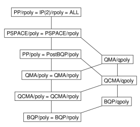
Figure 1: Known containments among classical and quantum advice classes.

Figure 1 shows the known relationships among deterministic, randomized, and quantum advice classes, in light of this paper’s results.  We still know remarkably little about quantum advice, compared to other computational resources.  But our results provide new evidence for a general hypothesis: that if you’re strong enough to squeeze an exponential amount of advice out of a quantum state, then you’re also strong enough to squeeze an exponential amount of advice out of a probability distribution.

We end with some open problems.

• Can we find a counterexample to the quantum advice hypothesis?  What about $\mathsf{QMA}\left(2\right)$, or $\mathsf{QMA}\left(k\right)$ for $k>2$, or $\mathsf{QS}_{2}^{p}$?  Currently, we do not even know whether $\mathsf{QMA}\left(2\right)\mathsf{/rpoly}=\mathsf{ALL}$; this seems related to the difficult open question of amplification for $\mathsf{QMA}\left(2\right)$ (see Kobayashi et al. [8]).

• Is there a class $\mathcal{C}$ such that $\mathcal{C}\mathsf{/rpoly}\neq\mathcal{C}\mathsf{/poly}$ but $\mathcal{C}\mathsf{/rpoly}\neq\mathsf{ALL}$?

• Can we tighten the $\Omega\left(N/\log^{2}N\right)$ lower bound of Theorem 6 to $\Omega\left(N\right)$?  One approach would be to tighten Lemma 15, by generalizing the in-place $\mathsf{QMA}$ amplification of Marriott and Watrous [10].

• Can we improve the containment $\mathsf{QMA/qpoly}\subseteq\mathsf{PSPACE/poly}$ to $\mathsf{QMA/qpoly}\subseteq\mathsf{PP/poly}$?  Alternatively, can we construct an oracle (possibly a ‘quantum oracle’ [3]) relative to which $\mathsf{QMA/qpoly}\not\subset\mathsf{PostBQP/poly}$?  This would indicate that the upper bound of $\mathsf{PSPACE/poly}$ might be difficult to improve.

6 . Acknowledgments

Greg Kuperberg collaborated in the research project of which this paper was an offshoot, and I am grateful to him for comments and advice, as well as for several observations including Proposition 16.  I also thank Oded Regev for first suggesting to me the problem of proving an upper bound on $\mathsf{QMA/qpoly}$; Ashwin Nayak and Hirotada Kobayashi for pointing out errors in an earlier version of Section 4.1; Harumichi Nishimura for helpful discussions; Jon Yard for pointing out a gap in an earlier version of Section 3.3; and Ronald de Wolf and the anonymous reviewers for comments on the manuscript.

7 . Appendix: Other Complexity Results

The purpose of this appendix is to show that, in upper-bounding $\mathsf{QMA/qpoly}$, the computational difficulty really does arise from the need to handle quantum advice and quantum witnesses simultaneously: if either or both are “dequantized,” then the upper bound of $\mathsf{PSPACE/poly}$ can be improved.  In particular, and in increasing order of nontriviality, Theorem 17 will show that $\mathsf{MA/rpoly}=\mathsf{MA/poly}$ (and likewise that $\mathsf{QCMA/rpoly}=\mathsf{QCMA/poly}$), Theorem 19 will show that $\mathsf{QMA/rpoly}=\mathsf{QMA/poly}$, and Theorem 20 will show that $\mathsf{QCMA/qpoly}\subseteq\mathsf{PP/poly}$.

First, however, let us make a cautionary observation, which illustrates why such upper bounds cannot be blithely assumed.  Recall that $\mathsf{MA}_{\mathsf{EXP}}$ is the exponential-time analogue of $\mathsf{MA}$.

Proposition 16

$\mathsf{MA}_{\mathsf{EXP}}\mathsf{/rpoly}=\mathsf{ALL}$.

Proof. Given an arbitrary Boolean function $f:\left\{0,1\right\}^{n}\rightarrow\left\{0,1\right\}$, an honest Merlin’s message will consist of the truth table of $f$, while the randomized advice will consist of an $O\left(n\right)$-bit fingerprint of the truth table.   

We can also “scale down” Proposition 16 by an exponential, to obtain $\mathsf{MA/poly}\subseteq\mathsf{MA/rl{}og}$.  More explicitly, in the $\mathsf{MA/rl{}og}$ simulation, an honest Merlin’s message will contain the advice $s$ to the $\mathsf{MA/poly}$ machine, while the $\mathsf{rl{}og}$ advice will consist of an $O\left(\log n\right)$-bit fingerprint of $s$.

We next show that $\mathsf{MA/rpoly}=\mathsf{MA/poly}$.  Combined with the above observation, this result has the surprising implication that

$$\mathsf{MA/rl{}og}=\mathsf{NP/poly}=\mathsf{MA/poly}=\mathsf{MA/rpoly.}$$

In other words, for an $\mathsf{MA}$ machine, $\operatorname*{poly}\left(n\right)$ bits of randomized advice are no more powerful than $\log\left(n\right)$ bits.

Theorem 17

$\mathsf{MA/rpoly}=\mathsf{MA/poly}$.

Proof. Let $L$ be a language in $\mathsf{MA/rpoly}$, and let $\mathcal{A}\left(x,r,z\right)$ be Arthur’s verification algorithm run on input $x$, advice string $r$, and witness $z\in\left\{0,1\right\}^{w\left(n\right)}$, for some polynomial $w$.  (We assume without loss of generality that Arthur is deterministic, since the randomized advice can provide his coins.)  Also, let $\mathcal{D}$ be the distribution from which $r$ is drawn.  Then for all $x\in L$, there exists a $z$ such that

$$\Pr_{r\in\mathcal{D}}\left[\mathcal{A}\left(x,r,z\right)\text{ accepts}\right]\geq\frac{2}{3},$$

whereas for all $x\notin L$ and all $z$,

$$\Pr_{r\in\mathcal{D}}\left[\mathcal{A}\left(x,r,z\right)\text{ accepts}\right]\leq\frac{1}{3}.$$

Let $R=\left(r_{1},\ldots,r_{p\left(n\right)}\right)$ be a $p\left(n\right)$-tuple of independent samples from $\mathcal{D}$, for some $p\left(n\right)=\Theta\left(n+w\left(n\right)\right)$.  Then there exists a boosted verifier $\mathcal{A}_{\ast}$ such that for all $x\in L$, there exists a $z$ such that

$$\Pr_{R\in\mathcal{D}^{p\left(n\right)}}\left[\mathcal{A}_{\ast}\left(x,R,z\right)\text{ accepts}\right]\geq 1-\frac{1}{2^{n}2^{w\left(n\right)}},$$

whereas for all $x\notin L$ and all $z$,

$$\Pr_{R\in\mathcal{D}^{p\left(n\right)}}\left[\mathcal{A}_{\ast}\left(x,R,z\right)\text{ accepts}\right]\leq\frac{1}{2^{n}2^{w\left(n\right)}}.$$

So by a simple counting argument, there exists a fixed advice string $R$ such that for all $x\in L$, there exists a $z$ such that Arthur accepts; whereas for all $x\notin L$ and all $z$, Arthur rejects.   

Indeed, using the same techniques we can show that

$$\mathsf{QCMA/rl{}og}=\mathsf{QCMA/ql{}og}=\mathsf{QCMA/poly}=\mathsf{QCMA/rpoly}.$$

Next we want to show a somewhat harder result, that $\mathsf{QMA/rpoly}=\mathsf{QMA/poly}$.  To do so we will need the following theorem of Marriott and Watrous.

Theorem 18 (Marriott and Watrous [10])

The error probability in any $\mathsf{QMA}$ protocol can be made exponentially small without increasing the size of Merlin’s quantum witness.

We can now prove the analogue of Theorem 17 for $\mathsf{QMA}$.

Theorem 19

$\mathsf{QMA/rpoly}=\mathsf{QMA/poly}.$

Proof. Given a language $L\in\mathsf{QMA/rpoly}$, let $\mathcal{D}$ be the distribution from which Arthur’s advice is drawn, and let $\mathcal{Q}\left(x,r,\left|\varphi\right\rangle\right)$ be Arthur’s verification algorithm run on input $x$, advice string $r$, and witness $\left|\varphi\right\rangle\in\mathcal{H}_{2}^{\otimes w\left(n\right)}$.  Then for all $x\in L$, there exists a $\left|\varphi\right\rangle$ such that

$$\Pr_{r\in\mathcal{D}}\left[\mathcal{Q}\left(x,r,\left|\varphi\right\rangle\right)\text{ accepts}\right]\geq\frac{2}{3},$$

whereas for all $x\notin L$ and all $\left|\varphi\right\rangle$,

$$\Pr_{r\in\mathcal{D}}\left[\mathcal{Q}\left(x,r,\left|\varphi\right\rangle\right)\text{ accepts}\right]\leq\frac{1}{3}.$$

Here the probability is taken over $\mathcal{Q}$’s internal randomness as well as $r$.

By Theorem 18, we can make the error probability exponentially small without increasing the size of $\left|\psi\right\rangle$.  So let $R=\left(r_{1},\ldots,r_{p\left(n\right)}\right)$ be a $p\left(n\right)$-tuple of independent samples from $\mathcal{D}$, for some $p\left(n\right)=\Theta\left(n+w\left(n\right)\right)$.  Then there exists a boosted verifier $\mathcal{Q}_{\ast}$ such that for all $x\in L$, there exists a $\left|\varphi\right\rangle$ such that

$$\Pr_{R\in\mathcal{D}^{p\left(n\right)}}\left[\mathcal{Q}_{\ast}\left(x,R,\left|\varphi\right\rangle\right)\text{ accepts}\right]\geq 1-\frac{1}{2^{n}2^{3w\left(n\right)}},$$

whereas for all $x\notin L$ and all $\left|\varphi\right\rangle$,

$$\Pr_{R\in\mathcal{D}^{p\left(n\right)}}\left[\mathcal{Q}_{\ast}\left(x,R,\left|\varphi\right\rangle\right)\text{ accepts}\right]\leq\frac{1}{2^{n}2^{3w\left(n\right)}}.$$

So by a simple counting argument, there exists a fixed advice string $R_{1}$ such that for all $x\in L$, there exists a $\left|\varphi\right\rangle$ such that Arthur accepts with probability at least $1-2^{-3w\left(n\right)}$.  However, we still need to handle the case $x\notin L$.  Since the number of states $\left|\varphi\right\rangle\in\mathcal{H}_{2}^{\otimes w\left(n\right)}$ with small pairwise inner product is doubly exponential, a naïve counting argument no longer works.  Instead, observe that there exists a fixed advice string $R_{0}$ such that for all $x\notin L$ and all computational basis states $\left|z\right\rangle$ with $z\in\left\{0,1\right\}^{w\left(n\right)}$,

$$\Pr\left[\mathcal{Q}_{\ast}\left(x,R_{0},\left|z\right\rangle\right)\text{ accepts}\right] \leq 2^{n}2^{w\left(n\right)}\cdot\frac{1}{2^{n}2^{3w\left(n\right)}}$$

$$=\frac{1}{2^{2w\left(n\right)}}.$$

Now suppose by contradiction that there exists a $\left|\varphi\right\rangle$ such that

$$\Pr\left[\mathcal{Q}_{\ast}\left(x,R_{0},\left|\varphi\right\rangle\right)\text{ accepts}\right]>\frac{1}{3}.$$

Then

$$\Pr\left[\mathcal{Q}_{\ast}\left(x,R_{0},I\right)\text{ accepts}\right]>\frac{1}{3}\cdot\frac{1}{2^{w\left(n\right)}},$$

where

$$I=\frac{1}{2^{w\left(n\right)}}\sum_{z\in\left\{0,1\right\}^{w\left(n\right)}}\left|z\right\rangle\left\langle z\right|$$

is the maximally mixed state on $w\left(n\right)$ qubits.  But this implies that there exists a basis state $\left|z\right\rangle$ such that

$$\Pr\left[\mathcal{Q}_{\ast}\left(x,R_{0},\left|z\right\rangle\right)\text{ accepts}\right]>\frac{1}{3}\cdot\frac{1}{2^{w\left(n\right)}},$$

which yields the desired contradiction.  Finally, by a union bound, there exists a fixed advice string $R$ that combines the properties of $R_{0}$ and $R_{1}$.   

7.1 . Upper-Bounding QCMA/qpoly

We now show that $\mathsf{QCMA/qpoly}\subseteq\mathsf{PP/poly}$.  Conceptually, the proof is similar to the proof that $\mathsf{QMA/qpoly}\subseteq\mathsf{PSPACE/poly}$, but with three differences.  First, since the witnesses are now classical, they can be provided to the simulating machine as part of the advice.  Second, since the witnesses are provided, there is no longer any need to try exponentially many random witnesses.  Indeed, this is what improves the upper bound from $\mathsf{PSPACE/poly}$ to $\mathsf{PP/poly}$.  And third, we can no longer exploit the fact that $\mathsf{BQPSPACE/qpoly}=\mathsf{PSPACE/poly}$, in order to split the proof neatly into a “de-Merlinization” part (which is new) and an “advice” part (which follows from earlier work of Aaronson [1]).  Instead, we need to generalize the machinery from [1] to the $\mathsf{QCMA}$ setting.

Theorem 20

$\mathsf{QCMA/qpoly}\subseteq\mathsf{PP/poly}$.

Proof. Let $L$ be a language in $\mathsf{QCMA/qpoly}$, and let $L\left(x\right)=1$ if $x\in L$ and $L\left(x\right)=0$ otherwise.  Also, let $\mathcal{Q}$ be a verifier for $L$, which takes a $a$-qubit quantum advice state $\left|\psi\right\rangle$ and $w$-bit classical witness $z$ for some polynomials $a$ and $w$ (for convenience, we omit the dependence on $n$).  Then the first step is to replace $\mathcal{Q}$ by an amplified verifier $\mathcal{Q}_{\ast}$, which takes an $A$-qubit advice state $\left|\Psi\right\rangle:=\left|\psi\right\rangle^{\otimes\ell}$, where $A=a\ell$ and $\ell=O\left(\log a\right)$.  As a result, $\mathcal{Q}_{\ast}$ has completeness and soundness errors $1/A^{4}$.

Let $\mathcal{Q}_{\ast}\left(x,\rho,z\right)$ be shorthand for $\mathcal{Q}_{\ast}$ run with input $x$, advice $\rho$, and witness $z$.  Then given $x$, our goal is to simulate $\mathcal{Q}_{\ast}\left(x,\left|\Psi\right\rangle,z\left(x\right)\right)$, where $z\left(x\right)$ is an optimal witness for $x$.  We will do so using a $\mathsf{PP/poly}$ machine $\mathcal{M}$.  The classical advice to $\mathcal{M}$ will consist of a “Darwinian training set” $\left(x_{1},z_{1}\right),\ldots,\left(x_{T},z_{T}\right)$ for $T=O\left(A\right)$, together with $L\left(x_{t}\right)$ for every $t\in\left\{1,\ldots,T\right\}$.  Here each $x_{t}\in\left\{0,1\right\}^{n}$ is an input and each $z_{t}\in\left\{0,1\right\}^{w}$ is its corresponding witness.  Given this advice, $\mathcal{M}$ runs the following procedure to compute $L\left(x\right)$.

let $\rho:=I_{A}$ be the maximally mixed state on $A$ qubits

for $t:=1$ to $T$

let $\left|b\right\rangle$ be a qubit initialized to $\left|0\right\rangle$

run $\mathcal{Q}_{\ast}\left(x_{t},\rho,z_{t}\right)$, and CNOT the output into $\left|b\right\rangle$

run $\mathcal{Q}_{\ast}^{-1}\left(x_{t},\rho,z_{t}\right)$ to uncompute garbage

measure $\left|b\right\rangle$, and postselect on observing $b=L\left(x_{t}\right)$

next $t$

for all $z\in\left\{0,1\right\}^{w}$,

let $\lambda_{z}$ be the probability that $\mathcal{Q}_{\ast}\left(x,\rho,z\right)$ accepts

if there exists a $z$ such that $\lambda_{z}\geq 2/3$, then accept

otherwise, if $\lambda_{z}\leq 1/3$ for all $z$, then reject

Let us first see why $\mathcal{M}$ can be simulated in $\mathsf{PP/poly}$.  The ‘for’ loop is just a postselected quantum computation, and can clearly be simulated by the result of Aaronson [2] that $\mathsf{PostBQP}=\mathsf{PP}$.  The one nontrivial step is to decide whether there exists a $z$ such that $\lambda_{z}\geq 2/3$, or whether $\lambda_{z}\leq 1/3$ for all $z$.  We do this as follows.  Let $\rho_{t}$ be the state of the advice register after the first $t$ postselection steps, conditioned on those steps succeeding.  We first amplify by repeating the ‘for’ loop $J=O\left(w\right)$ times, using a different advice register each time.  This yields $J$ copies of $\rho_{T}$.  We then replace $\mathcal{Q}_{\ast}\left(x,\rho_{T},z\right)$ by the doubly-amplified verifier $\mathcal{Q}_{\ast}^{\prime}\left(x,\rho_{T}^{\otimes J},z\right)$, which runs $\mathcal{Q}_{\ast}\left(x,\rho_{T},z\right)$ once for each of the $J$ advice registers, and returns the majority outcome.  Let $\lambda_{z}^{\prime}$ be the probability that $\mathcal{Q}_{\ast}^{\prime}\left(x,\rho_{T}^{\otimes J},z\right)$ accepts.  Then by a Chernoff bound, and assuming the constant in $J=O\left(w\right)$ is sufficiently large, we have reduced the problem to deciding whether

1. there exists a $z\in\left\{0,1\right\}^{w}$ such that $\lambda_{z}^{\prime}\geq 1-2^{-2w}$, or

2. $\lambda_{z}^{\prime}\leq 2^{-2w}$ for all $z$.

Now let

$$S:=\frac{1}{2^{w}}\sum_{z\in\left\{0,1\right\}^{w}}\lambda_{z}^{\prime}.$$

Then $S\geq 2^{-w-1}$ in case (1), whereas $S\leq 2^{-2w}$ in case (2).  So it suffices to give a $\mathsf{PP/poly}$ machine with $\alpha+\beta S$ accepting paths, for some positive constants $\alpha$ and $\beta$.  Our machine will simply do the following:

• Choose $z$ uniformly at random.

• Simulate a $\mathsf{PostBQP}$ computation that accepts with probability proportional to $\lambda_{z}^{\prime}$.

The reason this works is that the probability of the $T$ postselection steps in the ‘for’ loop all succeeding is independent of $z$.

It remains only to show $\mathcal{M}$’s correctness.  Let $p_{t}$ be the probability that the first $t$ postselection steps in the ‘for’ loop all succeed.  We choose the “training inputs” $x_{1},\ldots,x_{T}$ and witnesses $z_{1},\ldots,z_{T}$ in such a way that

1. $p_{t+1}\leq\frac{2}{3}p_{t}$ for all $t\in\left\{0,\ldots,T-1\right\}$.

2. $z_{t}$ is a valid witness for $x_{t}$ whenever $x_{t}\in L$, meaning that $\mathcal{Q}_{\ast}\left(x_{t},\left|\Psi\right\rangle,z_{t}\right)$ accepts with probability at least $1-1/A^{4}$.

3. There is no larger training set that satisfies (a) and (b).

Then it suffices to prove the following two claims:

1. $T=O\left(A\right)$ for all training sets that satisfy (a) and (b).

2. $\mathcal{M}$ correctly decides every input $x$, if we train it on some $\left(x_{1},z_{1}\right),\ldots,\left(x_{T},z_{T}\right)$ that satisfies (a), (b), and (c).

For Claim (i), notice that we can write the maximally mixed state $I$ as a mixture of $2^{A}$ orthonormal vectors

$$I=\frac{1}{2^{A}}\sum_{i=1}^{2^{A}}\left|\Psi_{i}\right\rangle\left\langle\Psi_{i}\right|,$$

where $\left|\Psi_{1}\right\rangle:=\left|\Psi\right\rangle$ is the “true” advice state.  We argue that the $\left|\Psi_{1}\right\rangle\left\langle\Psi_{1}\right|$ component must survive all $T$ postselection steps with high probability.  For if $x_{t}\notin L$, then $\mathcal{Q}_{\ast}\left(x_{t},\left|\Psi\right\rangle,z_{t}\right)$ accepts with probability at most $1/A^{4}$, while if $x_{t}\in L$, then $\mathcal{Q}_{\ast}\left(x_{t},\left|\Psi\right\rangle,z_{t}\right)$ rejects with probability at most $1/A^{4}$ by assumption (b).  So by Lemma 13, the probability of outputting the wrong answer on any of $\left(x_{1},z_{1}\right),\ldots,\left(x_{T},z_{T}\right)$, using $\left|\Psi\right\rangle$ as the advice, is at most $T\sqrt{1/A^{4}}=T/A^{2}$.  Hence

$$p_{T}\geq\frac{1}{2^{A}}\left(1-\frac{T}{A^{2}}\right).$$

On the other hand, $p_{t+1}\leq\frac{2}{3}p_{t}$ for all $t$ by assumption (a), and hence $p_{T}\leq\left(2/3\right)^{T}$.  Combining we obtain $T=O\left(A\right)$.

For Claim (ii), suppose by way of contradiction that $\mathcal{M}$ rejects some $x\in L$.  Then $\mathcal{Q}_{\ast}\left(x,\rho_{T},z\right)$ accepts with probability less than $2/3$ for all $z$.  But this implies that if we trained $\mathcal{M}$ on the enlarged set $\left(x_{1},z_{1}\right),\ldots,\left(x_{T},z_{T}\right),\left(x,z\right)$ for any $z$, then we would get $p_{T+1}\leq\frac{2}{3}p_{T}$, thereby contradicting the maximality of $T$.  Likewise, suppose $\mathcal{M}$ accepts some $x\notin L$.  Then there exists a “false witness” $\widehat{z}$ such that $\mathcal{Q}_{\ast}\left(x,\rho_{T},\widehat{z}\right)$ accepts with probability greater than $1/3$.  So if we trained $\mathcal{M}$ on the enlarged set $\left(x_{1},z_{1}\right),\ldots,\left(x_{T},z_{T}\right),\left(x,\widehat{z}\right)$, we would again get $p_{T+1}\leq\frac{2}{3}p_{T}$, contradicting the maximality of $T$.

References

- [1] S. Aaronson. Limitations of quantum advice and one-way communication. Theory of Computing, 1:1–28, 2005. quant-ph/0402095.
- [2] S. Aaronson. Quantum computing, postselection, and probabilistic polynomial-time. Proc. Roy. Soc. London, A461(2063):3473–3482, 2005. quant-ph/0412187.
- [3] S. Aaronson and G. Kuperberg. Quantum versus classical proofs and advice. In preparation, 2006.
- [4] A. Ambainis, A. Nayak, A. Ta-Shma, and U. V. Vazirani. Quantum dense coding and quantum finite automata. J. ACM, 49:496–511, 2002. Earlier version in ACM STOC 1999, pp. 376-383. quant-ph/9804043.
- [5] S. Goldwasser and M. Sipser. Private coins versus public coins in interactive proof systems. In Randomness and Computation, volume 5 of Advances in Computing Research. JAI Press, 1989.
- [6] A. Kitaev and J. Watrous. Parallelization, amplification, and exponential-time simulation of quantum interactive proof systems. In Proc. ACM STOC, pages 608–617, 2000.
- [7] H. Klauck. Quantum communication complexity. In Proc. Intl. Colloquium on Automata, Languages, and Programming (ICALP), pages 241–252, 2000. quant-ph/0005032.
- [8] H. Kobayashi, K. Matsumoto, and T. Yamakami. Quantum Merlin-Arthur proof systems: are multiple Merlins more helpful to Arthur? In ISAAC, pages 189–198, 2003. quant-ph/0306051.
- [9] R. E. Ladner. Polynomial space counting problems. SIAM J. Comput., 18:1087–1097, 1989.
- [10] C. Marriott and J. Watrous. Quantum Arthur-Merlin games. Computational Complexity, 14(2):122–152, 2005.
- [11] A. Nayak. Optimal lower bounds for quantum automata and random access codes. In Proc. IEEE FOCS, pages 369–377, 1999. quant-ph/9904093.
- [12] I. Newman. Private vs. common random bits in communication complexity. Inform. Proc. Lett., 39:67–71, 1991.
- [13] M. Nielsen and I. Chuang. Quantum Computation and Quantum Information. Cambridge University Press, 2000.
- [14] R. Raz. Quantum information and the PCP theorem. In Proc. IEEE FOCS, 2005. quant-ph/0504075.
- [15] J. Watrous. Space-bounded quantum complexity. J. Comput. Sys. Sci., 59(2):281–326, 1999.