Exactly solvable approximating models for Rabi Hamiltonian dynamics

Abstract

The interaction between an atom and a one mode external driving field is an ubiquitous problem in many branches of physics and is often modeled using the Rabi Hamiltonian. In this paper we present a series of analytically solvable Hamiltonians that approximate the Rabi Hamiltonian and compare our results to the Jaynes-Cummings model which neglects the so-called counter-rotating term in the Rabi Hamiltonian. Through a unitary transformation that diagonlizes the Jaynes-Cummings model, we transform the counter-rotating term into separate terms representing several different physical processes. By keeping only certain terms, we can achieve an excellent approximation to the exact dynamics within specified parameter ranges.

I Introduction

The Rabi Hamiltonian is an elegant model for describing the transitions between two electronic states coupled linearly to a single mode of a harmonic driving field within the dipole approximation. Because of its simplicity in form, it plays an important role in many areas of physics from condensed matter physics and biophysics to quantum optics Allen and Eberly (1975); Leggett et al. (1987). Given the apparent simplicity of this model and its wide range of applicability, it is not surprising that various aspects have been studied both analytically and numerically Wagner (1984); Debergh and Klimov (2001); Yabuzaki et al. (1974); Kus (1985); Müller et al. (1991); Bonci et al. (1991); Bonci and Grigolini (1992); Bishop et al. (1996); Feranchuk et al. (1996) Remarkably, exact solutions have not been thus far presented except for special cases Kus and Lewenstein (1986) even though it has been suggested that the problem may be solved exactly Reik and Doucha (1986); Reik et al. (1987) The Jaynes-Cummings model is a solvable approximation to the spin-boson model that neglects the counter-rotating term in the Rabi Hamiltonian Jaynes and Cummings (1963); Shore and Knight (1993). In general, it provides a reasonable approximation to the course-grained dynamics in the limit of weak coupling and weak field. For stronger fields and couplings, however, the model breaks down. While perturbative treatments can be used to some extent Zaheer and Zubairy (1988); Phoenix (1989), they give rise to fast oscillations and a dependence upon the phase of the initial state. Furthermore, it seems rather dangerous to introduce a term as a perturbation which may be as strong as terms already present in the unperturbed Hamiltonian.

In this paper, we present an alternative approach for including the counter-rotating terms into the Jaynes-Cummings model. We do this by transforming the counter-rotating term in the Rabi Hamiltonian to the basis in which the Jaynes-Cummings term is diagonal and then truncating the transformed counter-rotating operators to obtain a new series of exactly solvable models that are related by various symmetry operations. We then compare dynamics of the excited state survival probability for our approximating models to the Jaynes-Cummings model and to numerically exact solutions of the Rabi Hamiltonian and show that our approximate models do far better job in capturing both the long time decay and fine-structure in both the weak and strong field limits.

The rest of this paper is organized as follows. In Sec.II we obtain and justify the approximating Hamiltonians. In Sec. III eigenstates and eigenvalues of these Hamiltonians are found. Excited state survival probability for one of the approximating Hamiltonians and its comparison to the results for the Jaynes-Cummings and Rabi Hamiltonains are given in Sec. IV.

II Obtaining approximating Hamiltonians

The Rabi Hamiltonian describing interaction of a two level atom with a single-mode harmonic field can be written as ($\hbar=1$)

$$H=\frac{\omega}{2}\sigma_{z}+\nu a^{\dagger}a+g(\sigma^{+}+\sigma^{-})(a+a^{\dagger}).$$ (1)

Here $\sigma^{+}$ and $\sigma^{-}$ are spin-flip operators that satisfy

$$\sigma^{-}\sigma^{+}+\sigma^{+}\sigma^{-}=1,\qquad\sigma^{+}\sigma^{+}=\sigma^{-}\sigma^{-}=0,$$ (2)

$\sigma_{z}=2\sigma^{+}\sigma^{-}-1$, $a^{\dagger}$ and $a$ are the boson creation and annihilation operators, and $a^{\dagger}a=\hat{n}$ is the boson number operator. Hamiltonian (1) can be split into two parts as

$$H=H_{JC}+V,$$ (3)

where $H_{JC}$ is Jaynes-Cummings Hamiltonian

$$H_{JC}=\frac{\omega}{2}\sigma_{z}+\nu a^{\dagger}a+g(\sigma^{+}a+\sigma^{-}a^{\dagger})$$ (4)

and $V$ is the so-called counter-rotating term,

$$V=g(\sigma^{+}a^{\dagger}+\sigma^{-}a).$$ (5)

$H_{JC}$ can be brought to a diagonal form, $\tilde{H}_{JC}$, by a suitable unitary transformation,

$$\tilde{H}_{JC}=UH_{JC}U^{-1},$$ (6)

in which $U$ is a unitary operator of the form Yu et al. (1995)

$$U=e^{\sigma^{+}A-\sigma^{-}A^{\dagger}}.$$ (7)

In this paper we restrict our attention to the resonant case in which $\nu=\omega$ in Eq.(1). For this case, $A$ has the following simple form

$$A=\frac{\pi}{4\sqrt{\hat{n}+1}}a.$$ (8)

Here we use $\hat{n}$ for $a^{\dagger}a$ to simplify the notation. The unitary transformation operator in Eq. (7) can be brought into the following useful form,

$$U=\frac{1}{\sqrt{2}}+K(\hat{n})(1-\sigma_{z})+\sigma^{+}L(\hat{n})a-\sigma^{-}a^{\dagger}L(\hat{n}),$$ (9)

in which $K(\hat{n})$ and $L(\hat{n})$ are given by

$$K(\hat{n})=\left(\frac{\sqrt{2}-1}{2\sqrt{2}}\right)\delta(\hat{n}),\qquad L(\hat{n})=\frac{1}{\sqrt{2\hat{n}+2}}.$$ (10)

Here $\delta(\hat{n})$ is a projection operator on the ground state of the field. Unitary transformation generated by $U$ diagonalizes $H_{JC}$ as follows

$$\tilde{H}_{JC} = \frac{\omega}{2}\sigma_{z}+\omega{\hat{n}}$$ (11)

$$+\frac{g}{2}\left((\sigma_{z}+1)\sqrt{\hat{n}+1}+(\sigma_{z}-1)\sqrt{\hat{n}}\right)$$

in which the eigenstates are given by

$$|\theta_{n}^{\downarrow}\rangle=|\downarrow\rangle|n\rangle,\qquad|\theta_{n}^{\uparrow}\rangle=|\uparrow\rangle|n\rangle$$ (12)

where $|\downarrow\rangle$ and $|\uparrow\rangle$ are eigenstates of $\sigma_{z}$ with eigenvalues of $-1$ and $+1$, while $|n\rangle$ is an eigenstate of $\hat{n}$ with eigenvalue $n$.

We now consider how the unitary transformation that diagonalizes $H_{JC}$ transforms the total Hamiltonian (1).

$$\tilde{H}=UHU^{-1}=UH_{JC}U^{-1}+UVU^{-1}$$ (13)

The first term is diagonal and we focus our attention onto $\tilde{V}=UVU^{-1}$. $\tilde{V}$ can be written as a sum of four terms:

$$UVU^{-1}=\tilde{V}=\tilde{V}_{1}+\tilde{V}_{2}+\tilde{V}_{3}+\tilde{V}_{4}$$ (14)

where

$$\tilde{V}_{1} = g\left(\sigma^{+}F_{1}(\hat{n})a^{3}+\sigma^{-}(a^{\dagger})^{3}F_{1}(\hat{n})\right)$$

$$\tilde{V}_{2} = g\left(\sigma^{+}a^{\dagger}F_{2}(\hat{n})+\sigma^{-}F_{2}(\hat{n})a\right)$$

$$\tilde{V}_{3} = g\left(\sigma_{z}\left(F_{3}(\hat{n})a^{2}+(a^{\dagger})^{2}F_{3}(\hat{n})\right)\right)$$

$$\tilde{V}_{4} = g\left(F_{4}(\hat{n})a^{2}+(a^{\dagger})^{2}F_{4}(\hat{n})\right)$$ (15)

and $F_{1}$, $F_{2}$, $F_{3}$, and $F_{4}$ are expressed in terms of the $K$ and $L$ operators as

$$F_{1} = -L(\hat{n})L(\hat{n}+2)$$

$$F_{2} = \frac{1}{2}(1+2\sqrt{2}K(\hat{n}))$$

$$F_{3} = \frac{1}{2\sqrt{2}}\left(L(\hat{n})+L(\hat{n}+1)(1+2\sqrt{2}K(\hat{n}))\right)$$

$$F_{4} = \frac{1}{2\sqrt{2}}\left(L(\hat{n})-L(\hat{n}+1)(1+2\sqrt{2}K(\hat{n}))\right)$$

We can distinguish three types of terms in Eq.(II) based on the physical processes that they describe when acting on the $|\theta_{n}^{\uparrow\downarrow}\rangle$ states in Eq. (12). $\tilde{V}_{1}$ describes atomic excitation or relaxation though absorption or emission of three photons. $\tilde{V}_{2}$ describes the simultaneous excitation of the atom and creation of a photon or simultaneous relaxation of the atom and absorption of a photon. $\tilde{V}_{3}$ and $\tilde{V}_{4}$ correspond to creation or annihilation of two photons with no net change to the excitation state of the atom.

The question now becomes whether or not keeping only some terms in Eq. (14) leads to a solvable model and if so, is there a physical justification for keeping only those terms? Inspection of Eqs. (15) shows that there are two obvious cases,

$$\tilde{H}_{1}=\tilde{H}_{JC}+\tilde{V}_{1},\qquad\tilde{H}_{2}=\tilde{H}_{JC}+\tilde{V}_{2}$$ (17)

The reason for their solvability is the same as for the Jaynes-Cummings model, viz., there exist pairs of states such that the Hamiltonian can induce transitions only within each pair.

To determine if either $\tilde{H}_{1}$ or $\tilde{H}_{2}$ can be used to approximate $\tilde{H}$ when describing the system dynamics, we will use the same approach that justifies the use of the Jaynes-Cummings model as an approximation to the total Hamiltonian (1). Thus, we will write $\tilde{H}$ in the interaction picture using $\tilde{H}_{JC}$ as a free Hamiltonian and then analyze oscillatory behavior for different terms. Within the interaction picture, $\tilde{H}$ becomes,

$$\tilde{H}_{I}=e^{i\tilde{H}_{JC}t}\tilde{V}e^{-i\tilde{H}_{JC}t}.$$ (18)

Note that any operator that depends only on $\hat{n}$ and $\sigma_{z}$ remains unchanged in the interaction picture. Other operators that appear in Eq. (15) have the following interaction picture form

$$(\sigma^{-}(a^{\dagger})^{3})_{I} = \sigma^{-}(a^{\dagger})^{3}e^{iw_{1}t},$$ (19)

$$(\sigma^{+}a^{\dagger})_{I} = \sigma^{+}a^{\dagger}e^{iw_{2}t}.$$ (20)

$$(a^{\dagger})^{2}_{I} = (a^{\dagger})^{2}e^{iw_{3}t},$$ (21)

where

$$w_{1} = 2\omega-g(\sqrt{\hat{n}+3}+\sqrt{\hat{n}+1}),$$ (22)

$$w_{2} = 2\omega+g(\sqrt{\hat{n}+2}+\sqrt{\hat{n}}),$$ (23)

$$w_{3} = 2\omega+g(\sqrt{\hat{n}}-\sqrt{\hat{n}+2})+\frac{g}{2}(\sigma_{z}+1)$$ (24)

$$\times(\sqrt{\hat{n}+3}+\sqrt{\hat{n}+2}-\sqrt{\hat{n}+1}-\sqrt{\hat{n}}).$$

We can see that oscillation frequencies. $\omega_{i}$ are now operators. If we expand the states on which these operators act in terms of eigenstates of $\hat{n}$ and $\sigma_{z}$ then we can replace both $\hat{n}$ and $\sigma_{z}$ with their eigenvalues ($n$ for $\hat{n}$ and $\pm 1$ for $\sigma_{z}$) and $\omega_{i}$’s become $c$-numbers. For states with moderate occupation number $n$ we can approximate sums of square roots in Eqs. (22,23) as

$$\sqrt{n+3}+\sqrt{n+1}\approx 2\sqrt{n+1},$$

$$\sqrt{n+2}+\sqrt{n}\approx 2\sqrt{n+1}.$$ (25)

Differences of square roots in Eq. (24) are of order $1/\sqrt{n}$ and the terms involving these differences can be omitted if $g/\sqrt{n}\ll\omega$. This gives the following approximation for the effective frequencies

$$w_{1} \approx 2(\omega-g\sqrt{n+1})$$ (26)

$$w_{2} \approx 2(\omega+g\sqrt{n+1})$$ (27)

$$w_{3} \approx 2\omega$$ (28)

Comparing these effective frequencies, we can see the for $g>0$ we have $2|(\omega-g\sqrt{n+1})|<2\omega<2(\omega+g\sqrt{n+1})$ if $g\sqrt{n+1}<2\omega$. In this case operators appearing in Eq. (19) will have the slowest oscillating frequency. Similarly, if $g<0$, operators in Eq. (20) will have slower oscillating frequency then operators (19) and (21) if $-g\sqrt{n+1}<2\omega$ is satisfied. Thus, we may expect $\tilde{H}_{1}$ to give a reasonable description of the system dynamics for positive $g$ and $\tilde{H}_{2}$ for negative $g$ for specified ranges of parameters. Even though these approximations may be unsatisfactory in other regimes, we anticipate that some of the complex system dynamics that is present in the Rabi Hamiltonian will be manifest in our approximating Hamiltonians.

We now recall that the sign of $g$ in Eq. (1) can always be chosen as either negative or positive without the loss of generality. This is because there are two unitary transformation whose action on Hamiltonian (1) is equivalent to changing the sign of $g$. One is the space inversion transformation which changes the sign of $a$ and $a^{\dagger}$ and leaves $a^{\dagger}a$ invariant. (This transformation is generated by $\exp{(i\pi a^{\dagger}a)}$). Another is the transformation generated by $\exp{(i\frac{\pi}{2}(\sigma_{z}+1))}$ that changes the sign of $\sigma^{+}$ and $\sigma^{-}$ but leaves $\sigma_{z}$ invariant. Thus we can approximate Hamiltonian $\tilde{H}$ by either $\tilde{H}_{1}$ or $\tilde{H}_{2}$ depending on our choice of sign for $g$.

III Eigenstates and eigenvalues of the approximating Hamiltonians

First, we will consider Hamiltonian $\tilde{H}_{1}$. Its eigenstates and eigenvalues can be found along the same lines as for the Jaynes-Cummings model, i.e. by diagonalizing suitable two by two matrices. The eigenstates have the form

$$|\tilde{\phi}^{-}_{n}\rangle = A_{n}|\uparrow\rangle|n\rangle+B_{n}|\downarrow\rangle|n+3\rangle,\,\,\,\,{\rm and}$$

$$|\tilde{\phi}^{+}_{n}\rangle = B_{n}|\uparrow\rangle|n\rangle-A_{n}|\downarrow\rangle|n+3\rangle.$$ (29)

Here $n\geq 0$ and

$$A_{n}=\frac{1}{\sqrt{1+\alpha_{n}^{2}}},\qquad B_{n}=\frac{\alpha_{n}}{\sqrt{1+\alpha_{n}^{2}}},$$ (30)

where

$$\alpha_{n} = \frac{\mu_{n}}{\Delta_{n}+\eta_{n}},$$

$$\mu_{n} = g\sqrt{n+2},$$

$$\eta_{n} = 2\omega-g(\sqrt{n+1}+\sqrt{n+3}),$$

$$\Delta_{n} = \sqrt{\mu_{n}^{2}+\eta_{n}^{2}}.$$ (31)

Eigenvalues corresponding to eigenstates (29) are

$$\kappa^{\pm}_{n}=\frac{1}{2}((2n+3)\omega+g(\sqrt{n+1}-\sqrt{n+3})\pm\Delta_{n}).$$ (32)

Fig.1 gives $A^{2}(n)$ plotted as a continuous function of $n$ in the case weak coupling. It can be seen that for low-lying values of $n$, $A^{2}(n)$ is close to one indicating that in this region eigenstates (29) are similar to the Jaynes-Cummings eigenstates.

Figure 1: $A^{2}(n)$ as a continuous function of $n$ for weak coupling ($\omega=1,g=0.1$).

In addition to eigenstates (29), there are three special eigenstates of $\tilde{H}_{1}$ with eigenvalues

$$k_{0}=-\frac{\omega}{2},\qquad k_{1}=\frac{\omega}{2}-g,\qquad k_{2}=\frac{3\omega}{2}-\sqrt{2}g$$ (33)

All three are also eigenstates of $\tilde{H}_{JC}$ and are given by

$$|\tilde{\chi}_{0}\rangle=|\downarrow\rangle|0\rangle,\qquad|\tilde{\chi}_{1}\rangle=|\downarrow\rangle|1\rangle,\qquad|\tilde{\chi}_{2}\rangle=|\downarrow\rangle|2\rangle.$$ (34)

Moving on, we now consider eigenstates and eigenvalues of $\tilde{H}_{2}$. Its eigenstates have the form

$${|\tilde{\psi}^{-}_{n}\rangle} = C_{n}|\downarrow\rangle|n+1\rangle+D_{n}|\uparrow\rangle|n+2\rangle,$$

$${|\tilde{\psi}^{+}_{n}\rangle} = D_{n}|\downarrow\rangle|n+1\rangle-C_{n}|\uparrow\rangle|n+2\rangle$$ (35)

Here $n\geq 0$. We denote eigenvalues corresponding to states $|\phi_{n}^{\pm}\rangle$ by $\lambda_{n}^{\pm}$. Remarkably, the following relationship holds between coefficients $C_{n}$ and $A_{n}$ as well as $D_{n}$ and $B_{n}$ viewed as functions of the coupling parameter $g$,

$$C_{n}(g)=A_{n}(-g),\qquad D_{n}(g)=B_{n}(-g)$$ (36)

Similarly, we have for eigenvalues

$$\lambda_{n}^{\pm}(g)=\kappa_{n}^{\pm}(-g).$$ (37)

The validity of relations (36) and (37) can be easily checked if one writes for $\tilde{H}_{1}$ and $\tilde{H}_{2}$ explicit $2\times 2$ matrices whose diagonalization gives coefficents in Eq.(29) and Eq.(35) and eigenvalues for $\tilde{H}_{1}$ and $\tilde{H}_{2}$. For a given $n$, these matrices only differ by the sign in front of $g$.

As in the case of Hamiltonian $\tilde{H}_{1}$, there are three additional special eigenstates of $\tilde{H}_{2}$. Two of them have the same general form as eigenstates (35) but they do not have any simple relation (such as Eqs. (36,37)) to the special states of $\tilde{H}_{1}$. These two eigenstates are

$$|\tilde{\xi}^{-}\rangle=c|\downarrow\rangle|0\rangle+d|\uparrow\rangle|1\rangle,\qquad|\tilde{\xi}^{+}\rangle=d|\downarrow\rangle|0\rangle-c|\uparrow\rangle|1\rangle$$ (38)

Here, $c$ and $d$ are given by

$$c=\frac{1}{\sqrt{1+\gamma^{2}}},\qquad d=\frac{\gamma}{\sqrt{1+\gamma^{2}}},$$ (39)

where

$$\gamma = -\frac{g}{g+\sqrt{2}(\omega+\epsilon)},$$

$$\epsilon = \sqrt{g^{2}+\sqrt{2}g\omega+\omega^{2}}.$$ (40)

The corresponding eigenvalues are

$$l^{\pm}=\frac{1}{2}(\omega+\sqrt{2}g\pm 2\epsilon).$$ (41)

The third special state of $\tilde{H}_{2}$ is also an eigenstate of $\tilde{H}_{JC}$. It is given by

$$|\tilde{\xi}_{0}\rangle=|\uparrow\rangle|0\rangle$$ (42)

with eigenvalue

$$l_{0}=\frac{\omega}{2}+g$$ (43)

With the knowledge of eigenstates and eigenvalues of approximating Hamiltonians $\tilde{H}_{1}$ and $\tilde{H}_{2}$ we can calculate the time evolution of any observable. However, since observables of interest and initial states are given in the original untransformed picture, it is convenient to remain in this picture, in which case the time evolution is determined by

$$H_{1}=U^{-1}\tilde{H}_{1}U,\qquad H_{2}=U^{-1}\tilde{H}_{2}U$$ (44)

Explicit operator forms for $H_{1}$ and $H_{2}$ are given in the Appendix. Eigenstates of these operators are obtained by acting with $U^{-1}$ on states (29,34) in case of $H_{1}$ or states (35,38) in case of $H_{2}$. Eigenstates of $H_{1}$ are

$${|\phi^{-}_{n}\rangle} = \frac{1}{\sqrt{2}}|\downarrow\rangle\left(A_{n}|n+1\rangle+B_{n}|n+3\rangle\right)$$

$$+\frac{1}{\sqrt{2}}|\uparrow\rangle\left(-B_{n}|n+2\rangle+A_{n}|n\rangle\right),$$

$${|\phi^{+}_{n}\rangle} = \frac{1}{\sqrt{2}}|\downarrow\rangle\left(B_{n}|n+1\rangle-A_{n}|n+3\rangle\right)$$ (45)

$$+\frac{1}{\sqrt{2}}|\uparrow\rangle\left(A_{n}|n+2\rangle+B_{n}|n\rangle\right).$$

The special states of $H_{1}$ are given by

$$|\chi_{0}\rangle = |\downarrow\rangle|0\rangle,$$

$$|\chi_{1}\rangle = \frac{1}{\sqrt{2}}\left(|\downarrow\rangle|1\rangle-|\uparrow\rangle|0\rangle\right),$$

$$|\chi_{2}\rangle = \frac{1}{\sqrt{2}}\left(|\downarrow\rangle|2\rangle-|\uparrow\rangle|1\rangle\right).$$ (46)

For eigenstates of $H_{2}$ we have

$${|\psi^{-}_{n}\rangle} = \frac{1}{\sqrt{2}}|\downarrow\rangle\left(C_{n}|n+1\rangle+D_{n}|n+3\rangle\right)$$

$$+\frac{1}{\sqrt{2}}|\uparrow\rangle\left(D_{n}|n+2\rangle-C_{n}|n\rangle\right),$$

$${|\psi^{+}_{n}\rangle} = \frac{1}{\sqrt{2}}|\downarrow\rangle\left(D_{n}|n+1\rangle-C_{n}|n+3\rangle\right)$$ (47)

$$-\frac{1}{\sqrt{2}}|\uparrow\rangle\left(C_{n}|n+2\rangle+D_{n}|n\rangle\right).$$

The special eigenstates are

$$|\xi^{-}\rangle = |\downarrow\rangle\left(c|0\rangle+\frac{d}{\sqrt{2}}|2\rangle\right)+\frac{d}{\sqrt{2}}|\uparrow\rangle|1\rangle,$$

$$|\xi^{+}\rangle = |\downarrow\rangle\left(d|0\rangle-\frac{c}{\sqrt{2}}|2\rangle\right)-\frac{c}{\sqrt{2}}|\uparrow\rangle|1\rangle,$$

$$|\xi_{0}\rangle = \frac{1}{\sqrt{2}}|\downarrow\rangle|1\rangle+\frac{1}{\sqrt{2}}|\uparrow\rangle|0\rangle.$$ (48)

We can see that each of the states (45) and (47) is a superposition of four eigenstates of operators $\sigma_{z}$ and $\hat{n}$. In contrast, we may recall that eigenstates of $H_{JC}$ are superpositions of only two such states.

IV Dynamics of the atomic survival probability

We will now consider time evolution of the probability $P(t)$ for the atom to be exited if the initial state of the system given by $|\uparrow\rangle|f\rangle=|\uparrow,f\rangle$ where $|f\rangle$ is an arbitrary state of the field. $P(t)$ is expressed in terms of $\langle\sigma_{z}(t)\rangle$ as

$$P(t)=\frac{1}{2}(1+\langle\sigma_{z}(t)\rangle).$$ (49)

Let us consider the case of Hamiltonian $H_{1}$. Straightforward calculations using a complete set of eigenstates (45, 46) give for $P(t)$

$$P(t) = \frac{1}{2}+\Re e\Bigg{[}\sum_{n=0}^{\infty}\left(A_{n}A_{n+2}{F^{-}_{n+2}}^{*}{F^{+}_{n}}e^{i(\kappa^{-}_{n+2}-\kappa^{+}_{n})t}\right.$$ (50)

$$\left.-B_{n}A_{n+2}{F^{-}_{n+2}}^{*}{F^{-}_{n}}e^{i(\kappa^{-}_{n+2}-\kappa^{-}_{n})t}\right.$$

$$\left.\left.+A_{n}B_{n+2}{F^{+}_{n+2}}^{*}{F^{+}_{n}}e^{i(\kappa^{+}_{n+2}-\kappa^{+}_{n})t}\right.\right.$$

$$-\left.\left.B_{n}B_{n+2}{F^{+}_{n+2}}^{*}F_{n}^{-}e^{i(\kappa^{+}_{n+2}-\kappa^{-}_{n})t}\right)\right.$$

$$\left.+\frac{1}{\sqrt{2}}\left(A_{0}\langle 0|f\rangle{F^{-}_{0}}^{*}e^{i(\kappa^{-}_{0}-k_{1})t}\right.\right.$$

$$\left.\left.+B_{0}\langle 0|f\rangle{F^{+}_{0}}^{*}e^{i(\kappa^{+}_{0}-k_{1})t}\right.\right.$$

$$\left.\left.+A_{1}\langle 1|f\rangle{F^{-}_{1}}^{*}e^{i(\kappa^{-}_{1}-k_{2})t}\right.\right.$$

$$\left.+B_{1}\langle 1|f\rangle{F^{+}_{1}}^{*}e^{i(\kappa^{+}_{1}-k_{2})t}\right)\Bigg{]}.$$

Here

$$F^{-}_{n} = \langle\phi^{-}_{n}|\uparrow,f\rangle=\frac{1}{\sqrt{2}}(A_{n}\langle n|f\rangle-B_{n}\langle n+2|f\rangle),$$ (51)

$$F^{+}_{n} = \langle\phi^{+}_{n}|\uparrow,f\rangle=\frac{1}{\sqrt{2}}(A_{n}\langle n+2|f\rangle+B_{n}\langle n|f\rangle).$$ (52)

In order to qualitatively understand time dependence of $P(t)$ let us classify contributions from various terms in Eq. (50). All the terms in brackets have the form of time dependent exponentials preceded by a factor. Absolute values of these factors depend on the initial state of the field. The term in the second parentheses is due to the overlap of the initial state $|\uparrow,f\rangle$ with the special states (46). Its contribution is negligible for initial states with small $\langle 0|f\rangle$, $\langle 1|f\rangle$, $\langle 2|f\rangle$, and $\langle 3|f\rangle$ components. Oscillating exponentials that appear in the first parentheses can be divided into two groups - those involving differences of eigenvalues with the same superscripts and those involving differences of eigenvalues with the different superscripts.

Let us consider the $n$ dependence of $\kappa^{+}_{n+2}-\kappa^{+}_{n}$. We will again assume that states $|f\rangle$ have not too small average $\hat{n}$. Using explicit form of eigenvalues given by Eq. (32) it can be shown that

$$\kappa^{+}_{n+2}-\kappa^{+}_{n}=2\omega+{\cal O}\left(\frac{g}{\sqrt{n+1}}\right)$$ (54)

Hence, this difference can be approximated by $2\omega$ when $g/\sqrt{n+1}\ll\omega$ which holds for many couplings and initial states of interest. A similar result holds for $\kappa^{-}_{n+2}-\kappa^{-}_{n}$. Thus, the second and third terms in the first parentheses in Eq. (50) give primarily oscillating contributions with frequency of about $2\omega$.

Eigenvalue differences $\kappa^{-}_{n+2}-\kappa^{+}_{n}$ and $\kappa^{+}_{n+2}-\kappa^{-}_{n}$ have more complicated $n$ dependences. It can be shown that for states with typical $n\gg 1$ but such that $g\sqrt{n+1}\ll\omega$

$$\kappa^{-}_{n+2}-\kappa^{+}_{n} \approx 2g\sqrt{n+1},$$ (55)

$$\kappa^{+}_{n+2}-\kappa^{-}_{n} \approx 4\omega-2g\sqrt{n+1}.$$ (56)

These expressions allow to make connection with the standard Jaynes-Cummings model.

We showed earlier that for weak coupling coefficients $A_{n}$ are close to one and, therefore, $B_{n}$ are close to zero for moderate values of $n$ (Fig.1). Thus, the first term in the first parentheses in Eq. (50) is dominant for weak coupling for states with moderate average $\hat{n}$ values. Replacing $A_{n}\to 1$ and $B_{n}\to 0$ in Eqs.(52,LABEL:overlap2), approximating $\langle n+2|f\rangle$ with $\langle n|f\rangle$, using Eq. (55), and neglecting the terms in the second parentheses in Eq. (50) we obtain the survival probability for the resonant Jaynes-Cummings model Shore and Knight (1993)

$$P(t)\approx\frac{1}{2}\left(1+\sum_{0}^{\infty}|\langle n|f\rangle|^{2}\cos(2g\sqrt{n+1}\,t)\right).$$ (57)

Using Eq. (50), we can compare the survival probability $P_{AHM}(t)$ from our approximating Hamiltonian model to $P_{JCM}(t)$ from the Jaynes-Cummings model as well as the exact survival $P_{RH}(t)$ for the Rabi Hamiltonian (obtained by exact numerical integration of the corresponding Schrödinger equation). We treat both the Jaynes-Cummings model and the approximating Hamiltonian model as approximations of the Rabi Hamiltonian.

Fig. 2 shows survival probabilities $P(t)$ for the three models for the weak coupling case and when the initial state of the field is the number state with $n=6$. All models show qualitatively similar behavior of the Rabi type oscillations. However, $P_{RH}(t)$ never completely collapses (Fig. 2). This effect, although not so pronounced, is visible in the approximating Hamiltonian model as well. It can also be seen that the Rabi frequency for the Jaynes-Cummings model is very slightly larger then the oscillation frequency for the Rabi Hamiltonian whereas for the approximating Hamiltonian model it is slightly smaller.

Figure 2: Excited state survival probability for the Rabi Hamiltonian (RH), the approximating Hamiltonian model (AHM), and the Jaynes-Cummings model (JCM) ($\omega=1,g=0.1$) for the number initial state of the field with $n=6$.

Fig. 3 gives survival probabilities for the weak coupling case with the initial state of the field taken as the number state with $n=100$. We can see that in this case of the strong field both the Jaynes-Cummings model and the approximating Hamiltonian model deviate from the Rabi Hamiltonian. However, qualitatively, the approximating Hamiltonian model gives a better description. As the Rabi Hamiltonian, the approximating Hamiltonian model shows absence of complete collapse and strong deviation from simple oscillatory behavior.

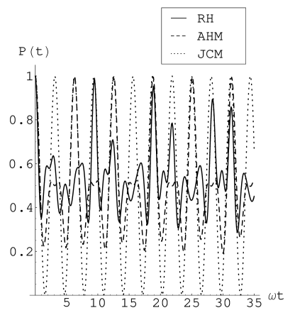
Figure 3: Excited state survival probability for the Rabi Hamiltonian, the approximating Hamiltonian model, and the Jaynes-Cummings model ($\omega=1,g=0.1$) for the number initial state of the field with $n=100$.

Taking the initial state of the field as a coherent leads to the results shown on Fig. 4 in the case of the weak coupling and weak field ($\langle n\rangle=4$). The approximating Hamiltonian model approximates the Rabi Hamiltonian better then the Jaynes-Cummings model because it account for fast oscillations in $P(t)$ with the frequency of about $2\omega$. However, the intensity of these oscillations is weaker compared to the Rabi Hamiltonian.

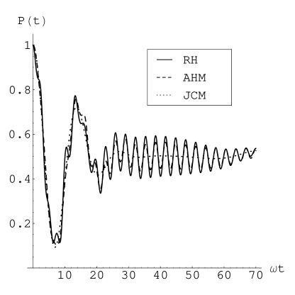
Figure 4: Excited state survival probability for the Rabi Hamiltonian, the approximating Hamiltonian model, and the Jaynes-Cummings model ($\omega=1,g=0.1$) for the coherent initial state of the field with $\alpha=2,(\langle n\rangle=4)$.

In the case of the strong coherent initial field (Fig. 5) The approximating Hamiltonian model again gives a better approximation to the Rabi Hamiltonian then the Jaynes-Cummings model. Both the Rabi Hamiltonian and the approximating Hamiltonian model show almost periodic revivals of $P(t)$ with no apparent weakening. In contrast to the Jaynes-Cummings model, both models do not have a region of nearly constant $P(t)$ before the onset of the second group of collapses and revivals that is present in the Jaynes-Cummings model.

Figure 5: Excited state survival probability for the Rabi Hamiltonian, the approximating Hamiltonian model, and the Jaynes-Cummings model ($\omega=1,g=0.1$) for the coherent initial state of the field with $\alpha=8,(\langle n\rangle=64)$.

It is easy construct explicit expression for $P(t)$ in the case of Hamiltonian $H_{2}$ using its eigenstates and eigenvalues. One can expect that due to the symmetry properties given by Eqs. (36,37) the following relationship will hold between $P(t)$ for $H_{1}$ and $P(t)$ for $H_{2}$ viewed as functions of $g$

$$P_{H_{1}}(g,t)\approx P_{H_{2}}(-g,t).$$ (58)

In general, the equality is not exact due contributions form the special states for Hamiltonians $H_{1}$ and $H_{2}$ for which there are no symmetry relations. We will not pursue investigation of $P_{H_{2}}(t)$ here since for $g<0$ it gives results that are qualitatively similar to $P_{H_{1}}$ for $g>0$.

V Conclusions

In this paper we present an approach that allows one to add extra terms to the Jaynes-Cummings model of an atom in an external field. These additional terms add complex oscillatory terms to the survival probability which become increasingly important as the field intensity is increased. By retaining select portions of the full counter-rotating term from the original Rabi Hamiltonian we obtain an analytically solvable model that compares favorably with the numerically exact survival probabilities from the Rabi Hamiltonian over a wide range of parameters even for relatively strong field strengths.

*

Appendix A

Explicit forms of Hamiltonians $H_{1}$ and $H_{2}$ are obtained by using Eqs. (9,44)

$$H_{1} = H_{JC}+\bigg{(}-\frac{g}{2}\sigma^{+}L(\hat{n})L(\hat{n}+2)a^{3}+\frac{g}{4}\sigma^{-}\big{(}1-\delta(\hat{n})\big{)}a$$ (59)

$$+\frac{g}{4\sqrt{2}}(1+\sigma_{z})L(\hat{n})a^{2}$$

$$-\frac{g}{4\sqrt{2}}(1-\sigma_{z})\big{(}1-\delta(\hat{n})\big{)}L(\hat{n}+1)a^{2}+h.c.\bigg{)}$$

$$H_{2} = H_{JC}+\bigg{(}-\frac{g}{2}\sigma^{+}L(\hat{n})L(\hat{n}+2)a^{3}+\frac{g}{4}\sigma^{-}\big{(}1+\delta(\hat{n})\big{)}a$$ (60)

$$-\frac{g}{4\sqrt{2}}(1+\sigma_{z})L(\hat{n})a^{2}$$

$$+\frac{g}{4\sqrt{2}}(1-\sigma_{z})\big{(}1+\delta(\hat{n})\big{)}L(\hat{n}+1)a^{2}+h.c.\bigg{)}$$

where operator $L(\hat{n})$ is defined in Eq. (10) and $h.c$ stands for Hermitian conjugate. We can see that in Hamiltonians $H_{1}$ and $H_{2}$, the counter-rotating terms are replaced by a number of terms involving various intensity dependent multi-photon transitions.

References

• Allen and Eberly (1975) L. Allen and J. H. Eberly, Optical Resonance and Two-Level Atoms (Wiley, New York, 1975).
• Leggett et al. (1987) A. J. Leggett, S. Chakravarty, A. T. Dorsey, M. P. A. Fisher, A. Garg, and W. Zwerger, Rev. Mod. Phys. 59, 1 (1987).
• Reik and Doucha (1986) H. G. Reik and M. Doucha, Phys. Rev. Lett. 57, 787 (1986).
• Reik et al. (1987) H. Reik, P. Lais, M. E. Stuzle, and M. Doucha, J. Phys. A 20, 6327 (1987).
• Kus and Lewenstein (1986) M. Kus and M. Lewenstein, J. Phys. A 19, 305 (1986).
• Wagner (1984) M. Wagner, J. Phys. A 17, 3409 (1984).
• Debergh and Klimov (2001) N. Debergh and A. B. Klimov, Int. J. Mod. Phys. A 16, 4057 (2001).
• Yabuzaki et al. (1974) T. Yabuzaki, S. Nakayama, Y. Murakami, and T. Ogawa, Phys. Rev. A 10, 1955 (1974).
• Kus (1985) M. Kus, Phys. Rev. Lett. 54, 1343 (1985).
• Müller et al. (1991) L. Müller, J. Stolze, H. Leschke, and P. Nagel, Phys. Rev. A 44, 1022 (1991).
• Bonci et al. (1991) L. Bonci, R. Roncaglia, B. J. West, and P. Grigolini, Phys. Rev. Lett. 67, 2593 (1991).
• Bonci and Grigolini (1992) L. Bonci and P. Grigolini, Phys. Rev. A 46, 4445 (1992).
• Bishop et al. (1996) R. F. Bishop, N. J. Davidson, R. M. Quick, and D. M. van der Walt, Phys. Rev. A 54, R4657 (1996).
• Feranchuk et al. (1996) I. D. Feranchuk, L. I. Komarov, and A. P. Ulyanenkov, J. Phys. A 29, 4035 (1996).
• Jaynes and Cummings (1963) E. T. Jaynes and F. W. Cummings, Proc. IEEE 51, 89 (1963).
• Shore and Knight (1993) B. W. Shore and P. L. Knight, J. Mod. Opt. 40, 1195 (1993).
• Zaheer and Zubairy (1988) K. Zaheer and M. S. Zubairy, Phys. Rev. A 37, 1628 (1988).
• Phoenix (1989) S. J. D. Phoenix, J. Mod. Opt. 36, 1163 (1989).
• Yu et al. (1995) S. Yu, H. Rauch, and Y. Zhang, Phys. Rev. A 52, 2585 (1995).