Almost Global Stochastic Feedback Stabilization of Conditional Quantum Dynamics ††thanks: Partially supported by the ministry of higher education of Italy (MIUR), under projects Control, Optimization and Stability of Nonlinear Systems: Geometric and Analitic Methods and Identification and Control of Industrial Systems.
Abstract
We propose several parametrization-free solutions to the problem of quantum state reduction control by means of continuous measurement and smooth quantum feedback. In particular, we design a feedback law for which almost global stochastic feedback stabilization can be proved analytically by means of Lyapunov techinques. This synthesis arises very naturally from the physics of the problem, as it relies on the variance associated with the quantum filtering process.
Keywords:
Quantum Feedback, Stochastic Stabilization, Nonlinear Stochastic Matrix Differential Equations, Quantum Filtering.
1 Introduction
Experimental techniques in quantum optics permit nowadays to continuously monitor and modify the dynamics of a cloud of cold atoms confined in an optical cavity [15]. The knowledge of the system state can be described by a conditional dynamical equation, the so-called Stochastic Master Equation (SME), obtained from a suitable quantum system-field interaction model by means of non-commutatitive filtering theory [31, 7], and based on monitoring the outgoing field from the cavity. The stochastic perturbation induced by the indirect measurement process produces an effective dynamical reduction model [1]. In other words, it makes the system state converge to one of the maximal information, pure states for the system physical observable interacting with the field.
If we have a second controllable field, acting as a time dependent Hamiltonian perturbation, then we can use the real-time estimate of the system state to modify the state reduction process. One possible use of such a feedback control strategy can be choosing to which pure state of the monitoring observable the system will converge. Beside possible interest for quantum measurement theory, the overall strategy can then be seen as a technique for engineering quantum state preparation.
From a control theoretic viewpoint, the problem is doubtless challenging. The SME is a nonlinear affine in control matrix Stochastic Differential Equation (SDE) living in the convex cone of positive semidefinite -dimensional Hermitian matrices. In the particular case of perfect measurement efficiency and maximal information on the initial condition, a SME turns out to be equivalent to a Stochastic Schrödinger Equation (SSE), i.e. a vector-valued, norm-preserving diffusion in [1, 8]. Influencing the open loop state reduction by means of the measurement is therefore a stochastic nonlinear feedback stabilization problem. Partial solutions to this problem were presented for example in [29] for 2 level SSE and, in more general terms, in [28] based on a (convex) numerical Lyapunov design. This last solution, however, suffers from scalability problems as the dimension of the system grows, since it is based on explicit parametrizations which grow with if is the dimension of the system.
For nonlinear (vector) SDE, most of the results on state feedback stabilization are due to Florchinger [12, 11, 13] (see also e.g. [9, 10, 5] for other possible approaches) and consists of extensions of Lyapunov-based techniques, like the Jurdjevic-Quinn condition, control Lyapunov function constructions, passivity-based methods and so on, to the stochastic case.
For our SME, these systematic construction methods have a limited success, and allow only to attain local stabilization in the particular case of SSE. The feedback that achieves it is the simple linear feedback already used for deterministic unitary feedback stabilization of quantum ensembles [3]. However, owing to the nature of the problem, local convergence results are of no practical interest. It is the structure of the problem itself that suggests how to improve the design: the state reduction encoded in the SME is “certified” by the variance of the continuous measurement process, a multiequilibrium Lyapunov-like function (with equilibria corresponding to the eigenvectors of the observable being measured) which is also a Morse function and can be used to enlarge the region of attraction of the controller. We shall in particular discuss two nonlinear feedback laws induced by the use of the variance, both more effective than the linear controller. Both allow for simple explicit proofs of convergence: one corresponds to a closed loop stochastic generator which is a sum of squares, the other to the square of a sum. The former achieves almost global stabilization for the perfect efficiency case, but cannot cancel all invariant sets of the dynamics in the more general SME and thus suffers from similar problems as the linear controller. The latter instead corresponds to a feedback stabilization design for the SME which is almost global, up to the isolated repulsive critical points (the remaining eigenvectors of the measured observable). This feedback strategy extends the idea of “symmetry breaking” enunciated in [28]. Indeed it works by using the uncontrollable part of the drift term to evade from the zero-control locus. We also show how the rate of convergence can be modified by tuning opportunely a pair of gains corresponding to the relative weights given to the controlled and uncontrolled parts of the stochastic generator.
2 Model formulation and background material
We need to recall some basics of quantum mechanics, quantum filtering and stochastic stability theory we will use later on. For an excellent introductory exposition to the statistical description of quantum systems see e.g. [21]. More details can be found in e.g. [22, 25] and references therein. For the theory of stochastic stability, main references are [4, 19], while for stochastic feedback stabilization we shall make use of the works of Florchinger [12, 11, 13]. Needless to say, the paper [28] presents similar control-theoretic perspective on most of the material mentioned below.
2.1 Quantum finite dimensional systems
In the standard statistical formulation of quantum mechanics [17, 26], to each quantum system is associated an Hilbert space , whose dimension depends essentially on the observable quantities we want to describe. In fact, physical observables are modelled as self-adjoint operators in the Hilbert space, the set of possible outcomes they can assume being their spectrum. In what follows, we will consider only observables with finite spectrum, thus represented as Hermitian matrices acting on .
Our knowledge of the system will be represented by a density matrix belonging to the convex set
The extremals of are the one dimensional orthogonal projections. These are called pure states, and are equivalent to unit vectors in up to an overall phase factor, by setting . We will use Dirac’s notation for vectors: , . Unit vectors in will be thus called state vectors. The usual notations and will be replaced by , .
Consider an observable and its spectral decomposition , where is a spectral family of orthogonal projectors summing to the identity. Assume one can perform an ideally instantaneous measurement of . The probability to obtain as an outcome is then given by
Thus, a density matrix determines also the expectation value of an observable
If is the observed outcome, the conditioned density matrix is given by the Lüders-von Neumann postulate as
| (1) |
We will assume throughout the paper to work in measurement units such that , where is the Plank constant divided by . In absence of measurements, the time evolution of an isolated quantum system is driven by the Hamiltonian , i.e., the energy observable, as specified by:
Notice that the evolution of the unobserved system is deterministic, and, if is pure, it is equivalent to the Scrödinger equation
Beside of these basic postulates and definitions, to tackle our main problem we will need more sophisticated tools to deal with continuous-time measurement and subsequent state conditioning.
2.2 Continuous Measurement and Filtering Equation
For explicit derivations and more detailed discussions of the following topics, we refer to e.g. [7, 6, 8, 28].
In the description of a classical uncertain system, observable quantities are represented by real random variables defined on a suitable probability space . The state of the system, i.e., our knowledge about it, is subsumed in the probability measure . The observables form a commutative algebra, .
The quantum setting presented in the previous section can be interpreted as a non commutative generalization of a classical, discrete probability space [21]. The need for non-commutativity emerges experimentally, motivating the standard axiomatic formulation of the theory and being essentially captured by the canonical commutation relations [26]. Briefly, quantum observables, or non commutative random variables, form a (generally non commutative) Von Neumann algebra and events are represented by orthogonal projections in the algebra. A generalized probability measure on is needed to compute probabilities of events.
The finite dimensional setting we are working in leads to a concrete representation of the above abstract notions. We can identify with Herm, and the set of generalized probability densities with , determining probabilities through .
One can then apply quantum filtering theory to obtain a conditional equation on for the dynamics [7]. It essentially plays the role of the classical Kushner-Stratonovich equation. Thus assume we are continuously monitoring the observable for the system of interest. In quantum optics, this can be accomplished e.g. for an angular momentum observable by an homodyne detection experimental setup [31]111In general, with homodyne detection one makes continuous-time measurements of generalized operators of the form: measuring the outgoing field from an optical cavity where we confine the system. The operator depends on the system-field interaction occurring in the cavity. We will specialize to the case of Hermitian operators .. Since the observed is time-invariant, we are conditioning the dynamics on the observation of a commuting quantum stochastic process, that leads to a dynamical equation driven by classical white noise (see e.g. [6]).
Let a (classical) probability space and a standard -valued Wiener process defined on this space. The homodyne detection measurement record can be written as the output of a stochastic dynamical system of the form:
| (2) |
where represents the efficiency of the measurement. Denote with the filtration associated to .
Then one can derive the filtering equation determining the conditional evolution of the state for the measurement record (2), the Quantum Filtering or Stochastic Master Equation (SME) à la Itô:
| (3) |
where represent the Hamiltonian part, with given by a drift and a (bilinear) control part , and are the drift and diffusion parts of the weak measurement performed along the observable . The parameter represents the strength of the measurement.
Here , the -valued solution of (3) given a constant initial condition , that can be written explicitly as
exists, is unique, adapted to the filtration and -invariant by construction, see [7, 28].
Considering (2) and (3) together, one can recognize the basic structure of a Kalman-Bucy filter. Since is the expectation of at time , in (2) plays the role of innovation process in a filtering model. Other correspondences with the classical setting have been discussed and highlighted in e.g. [27].
We denote by the infinitesimal generator à la Itô associated with the SME (3), written in a “symmetrized” fashion
| (4) |
Consider now the case of perfect detection efficiency . In this case, a pure remains pure throughout the evolution. In fact, recalling that if and only if , it suffices to prove the following.
Lemma 1
Consider (3) with a pure state and . Then
Proof. Using Ito’s rule, we have:
If the term disappears and
| (5) |
The assumption of starting with a pure state implies for example , and . Hence
| (6) |
and, likewise,
| (7) |
2.3 Elements of stochastic stability
Consider an equilibrium solution of (3), i.e. : .
Definition 1
The equilibrium of the SME (3) is said to be
We shall make use of the following Lyapunov conditions.
Theorem 1
Denote by the intersection of an open neighborhood with the set of density operators: . Assume a -valued with , and such that ( resp. ) . Then is locally stable (resp. locally asymptotically stable) in probability.
Since (3) is invariant in , the restriction of a full neighborhood to is not altering the standard proof of this result (reported for example in [19]).
Just like in the deterministic case, a well-established version of the LaSalle’s invariance principle provides the -limit set of a stable stochastic process.
Theorem 2
Since we have the semiclassical approximation with a control function, the SME (3) belongs to the class of stochastic affine in control nonlinear differential systems, for which a number of stabilizability conditions have been developed [11, 12, 13]. Call the infinitesimal generator of the uncontrolled part of the dynamics
where
Definition 2
The SME (3) satisfies a stochastic Lyapunov condition at if and a Lyapunov function such that for all for which the Lie derivative it is . The stochastic Lyapunov condition is almost global if is all of except for at most a finite number of isolated points.
When this condition is fulfilled, is said to be a stochastic control Lyapunov function for (3). Our feedback synthesis relies on this condition, but does not follow any of the standard constructions for control Lyapunov functions [12].
We shall instead make use of the following Jurjevic-Quinn type of stochastic stabilizability condition (see [12] Def. 3.5 and [11] Def. 3.1).
Theorem 3
Assume , and , , , such that
-
1.
;
-
2.
the set .
Then the feedback renders the equilibrium solution locally asymptotically stable in probability.
3 Continuous state reduction: the feedback stabilization problem
The problem we will discuss and solve can be stated as follows.
Problem 1
Find a smooth control law that (almost) globally stabilizes in probability the pure state of an -dimensional quantum system, whose dynamic is described by the filtering equation (3) conditioned by the continuous observation of an observable .
We shall propose several choices of as linear and nonlinear feedback laws based on the conditional estimate for the state at time . In the physics literature, this approach has been baptized bayesian feedback [30] and of course requires the real time integration of (3). Since is smooth and adapted to the filtration , the closed loop solution exists and is unique in a global sense.
The first feedback law proposed (§ 3.1) is linear and allows to achieve only local stabilizzability for the SSE (§ 3.2). If we choose a Lyapunov function that includes the variance of the measurement (§ 3.3), then two modifications of the linear law are easily identifiable and are presented in § 3.4 and § 3.5. The first one yields almost global asymptotic stability but only for the SSE, while with the second one we achieve almost global asymptotic stability in for the SME. The relation between rate of convergence and gain tuning for the latter feedback is discussed in § 3.6.
Let us first make suitable assumptions on and . In order for to be an equilibrium, assume is an eigenstate of and of . To avoid unnecessary complications, assume further that the spectrum of is non-degenerate and that . With this choice, it is always possible for example to fix a basis such that is diagonal and so are the free Hamiltonian and . We want to choose so that is rendered an attractor for the SME. Since the spectrum of is non-degenerate, state vectors other than , , , that are eigenstates of . When is diagonal, they correspond to diagonal density matrices with diagonal elements . Following the terminology of [3], we shall call these antipodal states of . Denote with the union of such antipodal points: . Finally, to avoid trivial cases, assume that is connected, i.e., that all transitions between energy levels are enabled by the control field.
3.1 A linear feedback controller
A natural choice for a Lyapunov function is the distance between density operators induced by the Hilbert-Schmidt norm [24]:
| (12) |
One clearly sees that in the stochastic differential (4) the quadratic part can be neglected since is linear in :
| (13) |
The non-Hamiltonian part vanishes because and commute and the cyclic property of trace holds (see the proof of Proposition 1): and
| (14) |
Hence in the SME (3) this stabilization design is concerned only with the unitary part of the evolution and has the natural solution
| (15) |
Since the closed loop system has
one needs to study the -limit set of (3) with the feedback (15). This is the difficult part of the linear feedback design (15). We certainly have the following for the set of (pure or mixed) diagonal density operators, call it (often call eigenensemble [32]).
Proposition 1
Proof. It suffices to notice that:
| (16) |
since
as any commutator under the trace operation. Similarly, . Thus, the only term affecting the dynamics is the diffusion term, which is also diagonal. Hence the diagonal set is invariant.
Since is a convex set, we have the following.
Corollary 1
In fact, the dynamics confined to is only a fluctuation and since the probability of collapse to the eigenstate is equal to , it is never 1 if .
3.2 Local stabilization of a class of Stochastic Schrödinger equations
Consider the case . As discussed in Section 2.2, the SME (3) is equivalent to the SSE (8) and the state space is . From the transversality of with respect to the set of diagonal Hermitian matrices (see Theorem E.2 of [14]), the intersection of with is just .
For this relevant particular case, one can show the following.
Theorem 4
Proof. In order to prove Theorem 4, we need a related deterministic result. Consider the deterministic unitary bilinear control system obtained from (3) in correspondence of
| (18) |
and its tangent linear system at
| (19) |
Lemma 2
Recall that strongly regular means nondegenerate and with all transition frequencies (i.e., all differences of eigenvalues) that are different. The proof of this Lemma is available in [3] (see also [23]). It essentially relies on the Jurdjevic-Quinn condition [18]: starting from the identity
compute sufficiently many derivatives
| (20a) | |||
| (20b) | |||
| (20c) | |||
The strong regularity condition of guarantees that all the commutators in (20) are linearly independent up to a number equal to , i.e., (17) holds with , implying the controllability of the linearization (19) and thus the local stabilizability of the original system (18). Since is a manifold (and not an Euclidean space like in [18]), the condition is only local.
Turning to the stochastic system (3) and the stochastic Jurdjevic-Quinn condition of Theorem 3, since we have a linear Lyapunov function, when computing in the quadratic part of does not appear:
| (21) |
Similarly,
| (22) |
and so on for , . Hence, in the case of strongly regular the stochastic Jurdjevic-Quinn condition holds whenever Lemma 2 holds, as the Lie algebra spanned by the commutators in is at least as large as the one spanned by the commutators appearing in the deterministic conditions 222Notice that since is linear, in Theorem 4 we are only concerned with the linear part of the infinitesimal generators and this allows to infer the stochastic Jurdjevic-Quinn condition directly in terms of the Lie algebra, just like in its deterministic counterpart. Redoing the computations above for the corresponding Stratonovich equation (for which Lie algebraic conditions can be made fully rigorous for any ) where the quadratic term in the drift, , is (in the case is traceless) one arrives at the same conclusion.. However, even when not strongly regular but is, the stochastic Jurdjevic-Quinn condition still holds as the terms
still provide the needed linearly independent commutators (see [2] for explicit recursive computations of the commutators involved). Since this is implied by (17), the proof is completed. The condition is local just like its deterministic counterpart.
Remark: Assume, without loss of generality, that . Then in order for (17) to hold it must be , i.e., the control Hamiltonian must “enable” all transitions from to all other eigenstates , .
When , the structure of the state space is larger than and in particular the transversality of the state space with respect to no longer holds, hence Theorem 4 does not apply.
3.3 A variance-based Lyapunov condition
The feedback (15) is the same linear controller used in [3] to study the deterministic stabilization problem with state feedback (corresponding to ). In that setting, its region of attraction does not correspond to the entire state space. In our stochastic problem, there is the additional requirement that the -limit set has to be invariant also to the flow of the diffusion part. We will exploit this feature, considering, instead of , the following candidate Lyapunov function:
| (24) |
Clearly , only in . The function in (24) is the variance of the filtering process along :
| (25) |
has the property of being a positive semidefinite Morse function on , i.e., a function whose critical points are nondegenerate [16] and can be used to attain a stochastic Lyapunov condition.
Theorem 5
Proof. To discuss the asymptotic properties of , it is useful to notice first that, using the cyclic property of the trace and Ito’s rule:
| (26) |
Thus, for the system (3) we have:
| (27) |
with the 3rd central moment.
From (24), (27) and (13), the stochastic differential à la Itô for is
| (28) |
Considering the zero-control behavior, notice that if the system state must be in an eigenstate of and hence . Thus is stationary for (27). The convergence to the eigenstates follows applying Theorem 1 to any bounded right interval of zero containing . In fact,
proves the convergence in probability of the variance to zero. Hence, for the closed loop system, looking at (28), everywhere, except at the other eigenvalues of and Definition 2 applies almost globally.
3.4 Almost global stabilization of the SSE by nonlinear feedback
Theorem 6
Assume . The feedback law
| (29) |
renders the equilibrium solution of the SSE (3) almost globally asymptotically stable in probability, with region of attraction given by .
Proof. The feedback (29) makes (28) into a negative semidefinite sum of squares:
| (30) |
Calling the set of critical points of : , from Theorem 2 we need to compute the -limit set of the closed loop inside . Since (30) is a sum of squares, must be a subset of . Since in , , , cannot be asymptotically stable in probability.
Remark: Notice that unlike Theorem 4, Theorem 6 does not require any special structure for (compare Remark following Theorem 4). In loose terms, one could say that while the design of Theorem 4 relies on a controllable linearization, in Theorem 6 uncontrollable, asymptotically stable modes are allowed in the linearization.
3.5 Almost global stabilization of the SME by nonlinear feedback
When , Proposition 1 and Corollary 1 still hold also with the feedback (29). Hence is not attracted to with probability 1. Although simulation results seem to suggest that with both the feedback laws (15) and (29) all non-diagonal density operators are attracted with probability 1 to , we do not see any clear way to prove it. The problem can however be solved in full generality by a different choice of feedback.
Theorem 7
The system (3) with feedback law
| (31) |
admits as equilibrium solution which is almost globally asymptotically stable. The only states in which are not attracted in probability to are its antipodal states.
Proof.
Consider still the Lyapunov function given in (24). It is easy to see that the nonlinear feedback (31) completes in (28) to a square:
Notice first that is a stationary point of both open and closed loop systems: . We need to show that cannot belong to the -limit set of the closed loop (with the exclusion of ) and that there is no subset of which can remain undriven for . The crucial difference with respect to (29) is that (31) implies . From Theorem 5, the stochastic Lyapunov condition holds true and guarantees almost globally. In particular, notice that everywhere in , hence cannot belong to the -limit set. In addition , i.e., the set of spurious critical points is evaded also by means of the control action. The other claim follow by the similar observation that the zero-feedback locus
is never invariant to outside .
Remark: If the domain of attraction of (31) is , the critical points of are automatically repulsive equilibria of the closed loop system. If for some , , then an arbitrarily small unitary open loop perturbation is enough to evade from .
3.6 Gain tuning and rate of convergence
The performances of the feedback design (31) can be improved by adding, and tuning appropriately, two different gains. Instead of (31), consider the following
| (32) |
with , . While corresponds to the usual feedback gain, can be thought of as a rescaling of the variance in the Lyapunov function (24):
The corresponding closed loop stochastic generator is then:
| (33) |
Proposition 2
Proof. From (33), for the closed loop system in , and finite , as the proof of Theorem 7 still applies. The limit behavior follows by inspection of (32).
Notice that tuning does not correspond to modulating the strength of the weak measurement .
The effect of is to change the influence of on the closed loop dynamics. In terms of the Hilbert-Schmidt norm , from (13), its close loop differential is given by
Since only the first term is sign definite, convergence in probability to the target state is guaranteed to be faster if we raise the gain (recall that was introduced only to perturb the “symmetry” of the problem).
4 Example: 2 level case
For , it is possible to give a simple pictorial description of the trajectories of the system, provided one chooses a real parametrization, like the triple representing the Bloch vector: , with the Pauli matrices. Consider the observable , its eigenstate and the Hamiltonian , . Since
the SME (3) in terms of the Bloch vector is
| (34) |
The Lyapunov functions are
hence
The feedback laws (15), (29) and (31) are, respectively,
| (35) | |||||
| (36) | |||||
| (37) |
for some , . In correspondence of and (36), the closed loop infinitesimal generator is the sum of squares
while for (37) it is the square of a sum
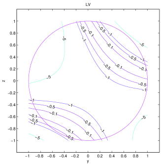
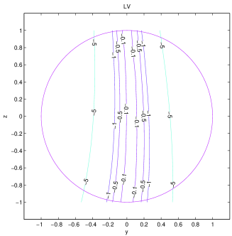
| (38) |
Looking at the closed loop dynamics, one sees that on the “line” of diagonal densities , for (35) and (36) the feedback is , the line itself is invariant and the dynamics driven only by the filtering term. This is no longer true for (37), as expected.
The level curves of (38) are visualized in Fig 1 for different choices of the parameters , . The figures shows that for that grows the locus tends to become aligned with the axis . The effect of raising instead is to increase the rate of convergence.

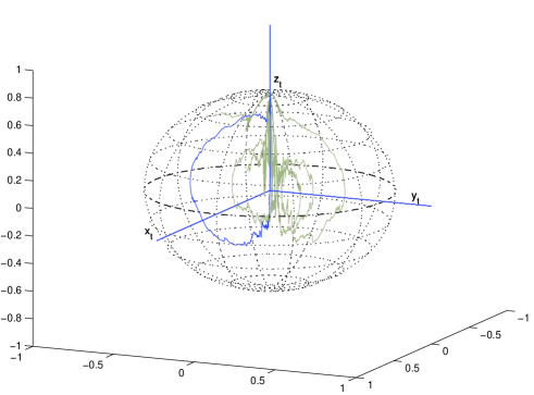
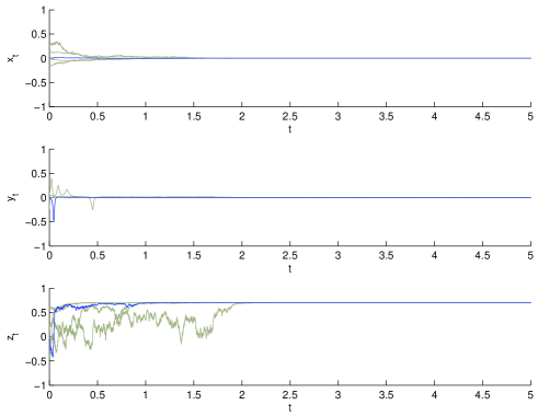
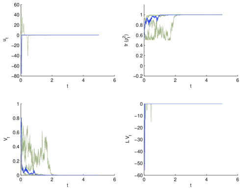
For the feedback (37), in Fig. 2 a few sample trajectories are plotted for different initial conditions (the boldface trajectory corresponds to , i.e., to the maximally mixed state). They are reproduced as versus time in Fig. 3. The corresponding time courses of , , and are shown in Fig. 4.
5 Conclusion
It is well known in Control Theory that finding a Lyapunov function for nonlinear systems is more an art than a systematic science, and that the knowledge about the physical process can provide the intuition necessary for this scope. The present work is nothing but a confirm of both these rules of thumb. We consider (some of) the standard design procedures available for the class of stochastic differential equations we deal with and show how they provide only a partial solution to our stabilization problem. Once we integrate this design with some physical insight on the structure of the SDE, however, the feedback synthesis becomes much more efficient and allows for a simple analytic demonstration regardless of the dimension of the system. In addition, since the Lyapunov function is a Morse function on the space of density operators, the feedback stabilization design guarantees global convergence up to a finite number of isolated and repulsive critical points.
Acknowledgements The authors would like to thank R. van Handel and S. Grivopoulos for useful discussions on the topic of this work.
References
- [1] S. L. Adler, D. C. Brody, T. A. Brun and L. P. Hughston. Martingale models for quantum state reduction, J. Phys. A: Math. Gen. 34 8795-8820, 2001.
- [2] C. Altafini. Controllability of quantum mechanical systems by root space decomposition of su(N). Journal of Mathematical Physics, 43:2051–2062, 2002.
- [3] C. Altafini. Feedback stabilization of quantum ensembles: a global convergence analysis on complex flag manifolds. Preprint arXiv:quant-ph/0506268, 2004.
- [4] L. Arnold. Stochastic Differential Equations: Theory and Applications. Krieger Publishing Company, Malabar, Florida, 1974.
- [5] S. Battilotti and A. De Santis. Stabilization in probability of nonlinear stochastic systems with guaranteed cost. SIAM J. Contr. Optim. 40: 1938–1964, 2002.
- [6] V. P. Belavkin. Nondemolition measurements and control in quantum dynamical systems. In Proceedings, Information Complexity and Control in Quantum Physics, Udine 1985 (A. Blaquiere, S. Diner and G. Lochak Eds.). pp.311-336. Springer-Verlag, Vienna-New York.
- [7] V. P. Belavkin. Quantum stochastic calculus and quantum nonlinear filtering. Journal of Multivariate Analysis, 42:171-201,1992.
- [8] L. Bouten, M. Guta and H. Maassen. Stochastic Schrodinger equations. MATH.GEN., 37, 3189, 2004
- [9] H. Deng and M. Krstic. Stochastic nonlinear stabilization. 1. A backstepping design. Systems & Control Lett. 32:151–159, 1997.
- [10] H. Deng and M. Krstic. Stochastic nonlinear stabilization. 2. Inverse optimality. Systems & Control Lett. 32:143–150, 1997.
- [11] P. Florchinger. A stochastic version of Jurdjevic-Quinn theorem. Stochastic Anal. Appl., 12:473–480, 1994.
- [12] P. Florchinger. Lyapunov-like techniques for stochastic stability. SIAM J. Control and Optimization, 33:1151–1169, 1995.
- [13] P. Florchinger. Feedback stabilization of affine in the control stochastic differential systems by the control Lyapunov function method. SIAM J. Control and Optimization, 35:500–511, 1997.
- [14] T. Frankel. The Geometry of Physics: An Introduction. Cambridge University Press, 2nd edition, 1999.
- [15] J. M. Geremia and J. K. Stockton and H. Mabuchi. Real-time quantum feedback control of atomic spin-squeezing. Science, 304:270-273, 2004.
- [16] V. Guillemin and A. Pollack Differential topology. Prentice-Hall Inc., Englewood Cliffs, N.J., 1974.
- [17] A. Holevo. Statistical Structure of Quantum Theory. Lecture Notes in Physics; Monographs: 67. Springer Verlag, 2001.
- [18] V. Jurdjevic and J. P. Quinn. Controllability and stability. Journal of Differential Equations, 28:381–389, 1978.
- [19] R. Z. Khas’minskiy. Stochastic Stability of Differential Equations. Sijthoff and Noordhoff, Alphen aan den Rijn, The Netherlands, 1980.
- [20] H. J. Kushner. Stochastic stability. In R. Curtain, editor, Stability of stochastic dynamical systems, Lecture Notes in Math., Vol. 294, pages 97–124. Springer, Berlin, 1972.
- [21] H. Maassen. Quantum probability applied to the damped harmonic oscillator, in Quantum Probability Communications XII 23-58, eds. S. Attal, J.M. Lindsay, World Scientific, Singapore 2003.
- [22] P. A. Meyer. Quantum Probability for Probabilists. Lecture Notes in Mathematics 1538. Springer Verlag, 1995.
- [23] M. Mirrahimi, P. Rouchon, and G. Turinici. Lyapunov control of bilinear Schrödinger equations. Automatic, in press, 2005.
- [24] M. A. Nielsen and I. L. Chuang. Quantum Computation and Quantum Information. Cambridge Univ. Press, 2000.
- [25] K. R. Parthasarathy. An Introduction to Quantum Stochastic Calculus, volume 85 of Monographs in Mathematics. Birkhauser, 1992.
- [26] J.J. Sakurai. Modern Quantum Mechanics. Addison-Wesley, revised edition, 1994.
- [27] A. C. Doherty, S. Habib, K. Jacobs, H. Mabuchi, S. M. Tan. Quantum Feedback Control and Classical Control Theory. Phys. Rev. A, 62, 012105, 2000 .
- [28] R. van Handel, J. K. Stockton and H. Mabuchi. Feedback Control of Quantum State Reduction. IEEE Trans. Automat. Control, 50, 768-780, 2005.
- [29] J. Wang and H. M. Wiseman. Feedback-stabilization of an arbitrary pure state of a two-level atom. Phys. Rev. A 64, 063810, 2001.
- [30] H. M. Wiseman, S. Mancini and J. Wang. Bayesian feedback versus Markovian feedback in a two-level atom, Phys. Rev. A 66, 013807, 2002.
- [31] H. M. Wiseman and G. J. Milburn. Quantum theory of optical feedback via homodyne detection. Phys. Rev. Lett.,70:5, 548-551, 1993.
- [32] K. Zyczkowski and W. Slomczyński. Monge metric on the sphere and geometry of quantum states. J. Phys. A, 34:6689, 2000.