Programmable quantum state discriminator by Nuclear Magnetic Resonance

Abstract

In this paper a programmable quantum state discriminator is implemented by using nuclear magnetic resonance. We use a two qubit spin-1/2 system, one for the data qubit and one for the ancilla (programme) qubit. This device does the unambiguous (error free) discrimination of pair of states of the data qubit that are symmetrically located about a fixed state. The device is used to discriminate both, linearly polarized states and elliptically polarized states. The maximum probability of the successful discrimination is achieved by suitably preparing the ancilla qubit. It is also shown that, the probability of discrimination depends on angle of unitary operator of the protocol and ellipticity of the data qubit state.

I I. Introduction

Researchers have studied the possibility of performing computations using quantum systems and conjectured that a machine based on quantum mechanical principles might be able to solve certain types of problems more efficiently than can be done on conventional computersfey ; ben ; deu . Later Lloyd proposed that such a quantum computer might be built from an array of coupled two state quantum systemsloy . Its theoretical possibility has generated a lot of enthusiasm for its experimental realizationpw ; deujoz ; gr ; gru ; db ; ic . In parallel with quantum computation, the related field of quantum information theory is developed, which forms the quantum analogue of classical information theory cov . Several techniques are being exploited for quantum computing and quantum information processing, including nuclear magnetic resonance nmr1 ; nmr2 ; nmr3 ; nmr4 ; nmr5 ; nmr6 ; nmr7 ; nmr8 .

Recently quantum state discrimination has been studied extensively in the context of quantum communication and quantum cryptography phil ; zh ; barr ; che ; che1 ; hel ; iva ; peres . Quantum state discrimination is the problem of determining the quntum state, given the constraint that it belongs to the previously specified set of non-orthogonal states. One of the characteristic features of quantum mechanics is that, it is impossible to devise a measurement that can distinguish non-orthogonal states perfectly ic . However one can distinguish them with a finite probability by appropriate measurement strategy. There are two different optimal strategies of discrimination: (i) Probabilistic discrimination (conclusive result, but error may appear) and (ii) Unambiguous discrimination(inconclusive result may appear, but no error). The unambiguous discrimination of two pure states was investigated by Ivanovic iva , and the optimal procedure was given by Peres peres . Cheffels and Barnett have generalized Peres’s solution to an arbitrary number of equally probable states which are related by a symmetry transformationche3 . The first experiment to discriminate two non-orthogonally polarized single photons states of light was done by Huttner et.alhut .

Quantum measurement is the final step of any quantum computation. In many situations the choice of an optimal measurement depends on the task to be performed. A quantum multimeter is a quantum measurement device which can perform a specific class of generalized measurements in such a way that each member of this class is selected by a particular quantum state of a programme register dus ; fil ; fiu ; paz ; ari . The parameters determining the character of quantum measurement can be encoded in a quantum state of a programme registerniel ; vid ; hil . Dusek et. al dus have shown that pair of non-orthogonal states of a qubit can be discriminated and the measurement to be done for this discrimination is decided by the state of the programme qubit (ancilla qubit). One can discriminate several pairs of states of a qubit by using the same protocoldus . Such a quantum device is known as quantum multimeter for the discrimination of pair of qubit states. Recently Dusek et. al dus1 have also demonstrated experimentally the possibility to control the discrimination process by the quantum state of ancilla qubit, in linear optics by performing the partial measurement in the Bell basis. Cryptographic applications of quantum state discrimination have been extensively studied in the literaturedus2 ; ham ; yon ; zhu .

Nuclear magnetic resonance (NMR) has played a leading role for practical demonstration of quantum algorithms and gates nmr1 ; nmr2 ; nmr3 ; nmr4 ; nmr5 ; nmr6 ; nmr7 ; nmr8 . . The unitary operators needed for implementation of these quantum circuits have mostly been realized using spin selective as well as transition selective radio frequency pulses and coupling evolution, utilizing spin-spin (J) or dipolar couplings among the spins nmr1 ; nmr2 ; nmr3 ; nmr4 ; nmr5 ; nmr6 ; nmr7 ; nmr8 . In this paper we demonstrate the implementation of quantum state discriminator which discriminates the pair of non orthogonal states as well as orthogonal states which are symmetric about a particular state, conditioned on the state of the ancilla qubit. We use spin selective pulses and evolution under J-coupling for the implementation. Projective measurement required for the discrimination is simulated by a method given by Collinscol . Our experimental results are in agreement with the theoretical resultsdus . To the best of our knowledge this is the first experimental demonstration of programmable quantum state discriminator by NMR.

In section(II), we discuss the theory of discrimination of both elliptically and linearly polarized states. Experimental details and results of different experiments are given in section(III). Results are concluded in section(IV). In the Appendix, unitary operators of ideal pulses are derived.

II II. Theory

The following protocol discriminates pair of elliptically polarized states of the data qubit unambiguously (error free). Let the two states $|\psi_{1}\rangle$ and $|\psi_{2}\rangle$ of the data qubit be (fig. 1a),

$$|\psi_{1}\rangle=(xcos\theta_{1}+iysin\theta_{1})|0_{D}\rangle\ +(xsin\theta_{1}-iycos\theta_{1})|1_{D}\rangle,$$

$$|\psi_{2}\rangle=(xcos\theta_{1}+iysin\theta_{1})|0_{D}\rangle\ -(xsin\theta_{1}-iycos\theta_{1})|1_{D}\rangle.$$ (1)

Ellipticity $(\epsilon)$ of the data qubit states is defined as, tan$(\epsilon)$=y/x. Here y=x corresponds to circularly polarized states and y=0 ($\epsilon$= 0) corresponds to linearly polarized states (fig. 1b). The protocol uses one ancilla (programme) qubit for the discrimination. A quantum circuit for the discrimination is shown in Fig. 2. In this circuit the first qubit is the data qubit ($|\psi_{D}\rangle$) and the second qubit is the ancilla qubit ($|\psi_{A}\rangle$). The data qubit can be either $|\psi_{1}\rangle$ or $|\psi_{2}\rangle$. The aim of the protocol (fig. 2) is to determine whether the data qubit is $|\psi_{1}\rangle$ or $|\psi_{2}\rangle$, knowing the angle between $|\psi_{1}\rangle$ and $|\psi_{2}\rangle$. It is shown that, a pair of data qubit states $|\psi_{1}\rangle$ and $|\psi_{2}\rangle$ can be discriminated by suitably preparing the ancilla qubit. One can switch the apparatus to work with several different pairs of data qubit states. In this paper we experimentally demonstrate the discrimination of both elliptically and linearly polarized states, and compare the results with simulations. In the following, we first describe the discrimination of elliptically polarized states and later the linearly polarized states.

Elliptically polarized states $|\psi_{1}\rangle$ and $|\psi_{2}\rangle$ (eqn. 1) can be re-written as,

$$|\psi_{1}\rangle=a_{1}|0\rangle+b_{1}|1\rangle,$$

$$|\psi_{2}\rangle=a_{1}|0\rangle-b_{1}|1\rangle,$$ (2)

where $a_{1}=xcos\theta_{1}+iysin\theta_{1}$ and $b_{1}=xsin\theta_{1}-iycos\theta_{1}$ are complex numbers, where by definition $x^{2}+y^{2}=1$.

$a_{1}$ and $b_{1}$ can also be written in polar form as,

$$a_{1}=e^{i\phi_{1}}cos(\eta)\hskip 14.22636ptand\hskip 14.22636ptb_{1}=e^{i\phi_{2}}sin(\eta),\hskip 8.5359ptwhere,$$ (3)

$$tan(\eta)=\frac{|b_{1}|}{|a_{1}|},\hskip 5.69046pt tan(\phi_{1}) =(\frac{ysin\theta_{1}}{xcos\theta_{1}}),\hskip 5.69046ptand\hskip 5.69046pttan(\phi_{2})=(\frac{-ycos\theta_{1}}{xsin\theta_{1}}).$$ (4)

Then $|\psi_{1}\rangle$ and $|\psi_{2}\rangle$ can be written as general states on the Bloch sphere ic ,

$$|\psi_{1}\rangle=cos(\eta)|0\rangle+e^{i\phi}sin(\eta)|1\rangle,$$

$$|\psi_{2}\rangle=cos(\eta)|0\rangle-e^{i\phi}sin(\eta)|1\rangle,$$ (5)

where $\phi=\phi_{2}-\phi_{1}$ with the overall phase ($e^{i\phi_{1}}$) being neglected.

Let the ancilla qubit (programme qubit) be,

$$|\psi_{A}\rangle=a_{2}|0\rangle+b_{2}|1\rangle,$$ (6)

where $a_{2}=xcos\theta_{2}+iysin\theta_{2}$ and $b_{2}=xsin\theta_{2}-iycos\theta_{2}$. To discriminate $|\psi_{1}\rangle$ and $|\psi_{2}\rangle$, the condition on $a_{2}$ and $b_{2}$ is derived as follows.

The total input state is $|\psi_{DA}\rangle$ = $|\psi_{D}\rangle\otimes|\psi_{A}\rangle$, where the data qubit $|\psi_{D}\rangle$ is either $|\psi_{1}\rangle$ or $|\psi_{2}\rangle$ (eqn. 2).

$$|\psi_{DA}\rangle=(a_{1}a_{2}|0_{D}0_{A}\rangle+a_{1}b_{2}|0_{D}1_{A}\rangle)\pm(b_{1}a_{2}|1_{D}0_{A}\rangle+b_{1}b_{2}|1_{D}1_{A}\rangle).$$ (7)

The sign of the second term in Eqn. (7) determines whether the data qubit is $|\psi_{1}\rangle$ or $|\psi_{2}\rangle$. The protocol for the discrimination requires a unitary transformation on $|\psi_{DA}\rangle$ given by dus ,

$$U=\pmatrix{cos(\alpha)&-sin(\alpha)&0&0\cr sin(\alpha)&cos(\alpha)&0&0\cr 0&0&1&0\cr 0&0&0&1},$$ (8)

where $\alpha$ is a fixed parameter which does not depend on the data and programme qubits states. The unitary operator given in Eqn. 8, is a rotation in the subspace spanned by $|0_{D}0_{A}\rangle$ and $|0_{D}1_{A}\rangle$, which is achieved here by two controlled-not gates and four single qubit gates (fig. 2), where the Single qubit gates are given by,

$$X=\pmatrix{0&1\cr 1&0},u1=\pmatrix{cos(\alpha/2)&sin(\alpha/2)\cr-sin(\alpha/2)&cos(\alpha/2)},u2=\pmatrix{cos(\alpha/2)&-sin(\alpha/2)\cr sin(\alpha/2)&cos(\alpha/2)},$$ (9)

And controlled-not(CNOT) gate is given by,

$$CNOT=\pmatrix{1&0&0&0\cr 0&1&0&0\cr 0&0&0&1\cr 0&0&1&0}.$$ (10)

After the application of the unitary transformation U(eqn. 8), the final state is,

$$U|\psi_{DA}\rangle=(a_{1}a_{2}cos\alpha-a_{1}b_{2}sin\alpha)|0_{D}0_{A}\rangle+(a_{1}a_{2}sin\alpha+a_{1}b_{2}cos\alpha)|0_{D}1_{A}\rangle\pm [b_{1}a_{2}|1_{D}0_{A}\rangle\ +b_{1}b_{2}|1_{D}1_{A}\rangle].$$ (11)

For successful discrimination of data qubit states $|\psi_{1}\rangle$ and $|\psi_{2}\rangle$, the condition on the coefficients of Eqn. (11) is,

$$(a_{1}a_{2}cos\alpha-a_{1}b_{2}sin\alpha)=b_{1}a_{2},$$ (12)

This yields,

$$U|\psi_{DA}\rangle=[b_{1}a_{2}|0_{D}0_{A}\rangle + (a_{1}a_{2}sin\alpha+a_{1}b_{2}cos\alpha)|0_{D}1_{A}\rangle]$$ (13)

$$\pm [b_{1}a_{2}|1_{D}0_{A}\rangle\ +b_{1}b_{2}|1_{D}1_{A}\rangle].$$ (14)

Equation (13) can be re-written as,

$$U|\psi_{DA}\rangle=\sqrt{2}b_{1}a_{2}|\pm\rangle+(a_{1}a_{2}sin\alpha+a_{1}b_{2}cos\alpha)|0_{D}1_{A}\rangle\pm b_{1}b_{2}|1_{D}1_{A}\rangle,$$ (15)

where $|\pm\rangle=1/\sqrt{2}(|0_{D}0_{A}\rangle\pm|1_{D}0_{A}\rangle)$.

If the final state (eqn. 14) contains state $|+\rangle$ then the initial state of the data qubit is $|\psi_{1}\rangle$ if the final state contains state $|-\rangle$ then the initial state of the data qubit is $|\psi_{2}\rangle$. Square of the coefficient ($\sqrt{2}b_{1}a_{2}$) of the state $|\pm\rangle$ is called the probability (P) of discrimination dus .

Equation (12) gives the condition on the ancilla qubit state. For example, when $\alpha=90^{o}$, $(b_{2}/a_{2})=-(b_{1}/a_{1})$ , and from Eqn.s 2 and 6 it is seen that $|\psi_{A}\rangle$=$|\psi_{2}\rangle$. However for other values of $\alpha$, $|\psi_{A}\rangle$ differs from $|\psi_{1}\rangle$ and $|\psi_{2}\rangle$. Hence $\alpha=90^{o}$ is a special case of Eqn. (12).

In NMR, the measurement is performed on an ensemble and the results are contained in the expectation values ($\langle\sigma_{x}\rangle$ and $\langle\sigma_{y}\rangle$) of Pauli spin matrices, which in the frequency space yield intensities of various transitions. From Eqn. (14) it is noted that the two transitions of the data qubit have different intensities. The $|0_{D}0_{A}\rangle\leftrightarrow|1_{D}0_{A}\rangle$ transition has the intensity $\pm b_{1}^{2}a_{2}^{2}$, and the $|0_{D}1_{A}\rangle\leftrightarrow|1_{D}1_{A}\rangle$ transition has the intensity $\pm(a_{1}a_{2}sin(\alpha)+a_{1}b_{2}cos(\alpha))b_{1}b_{2}$. To find whether the final state (eqn. 14) contains $|+\rangle$ or $|-\rangle$, one has to do the projective measurement on the state $|\pm\rangle$. To simulate projective measurement, we use a method given by Collins for an expectation value quantum search col ; kim . In our experiments, the goal of the projective measurement is to collapse the state of the ancilla qubit (given by equation 14) to $|0_{A}\rangle$ so that the data qubit gives only one peak which is the coherence of the superposition state $|\pm\rangle$ (or $|0_{D}0_{A}\rangle\leftrightarrow|1_{D}0_{A}\rangle$ transition). One can collapse the state of the ancilla qubit to $|0_{A}\rangle$ by adding two experiments (detection on the data qubit), one without controlled-$\sigma_{z}$ gate and one with controlled-$\sigma_{z}$ gate (fig. 2). Here the controlled-$\sigma_{z}$ gate is given by the unitary transformation,

$$\sigma_{z}^{c}=\pmatrix{1&0&0&0\cr 0&1&0&0\cr 0&0&1&0\cr 0&0&0&-1}.$$ (16)

Controlled-$\sigma_{z}$ gate inverts the sign of the state$|1_{D}1_{A}\rangle$. When $\sigma_{z}^{c}$ is applied after the unitary transformation U (eqn. 8), the final state (eqn. 14) becomes,

$$\sigma_{z}^{c}U|\psi_{DA}\rangle=\sqrt{2}b_{1}a_{2}|\pm\rangle+(a_{1}a_{2}sin\alpha+a_{1}b_{2}cos\alpha)|0_{D}1_{A}\rangle\mp b_{1}b_{2}|1_{D}1_{A}\rangle.$$ (17)

In the first experiment (eqn. 14), intensities of the data qubit transitions corresponding to $|0_{D}0_{A}\rangle\leftrightarrow|1_{D}0_{A}\rangle$ and $|0_{D}1_{A}\rangle\leftrightarrow|1_{D}1_{A}\rangle$ are, $\pm b_{1}^{2}a_{2}^{2}$ and $\pm(a_{1}a_{2}sin(\alpha)+a_{1}b_{2}cos(\alpha))b_{1}b_{2}$ respectively, whereas in the second experiment (eqn. 16) intensities are $\pm b_{1}^{2}a_{2}^{2}$ and $\mp(a_{1}a_{2}sin(\alpha)+a_{1}b_{2}cos(\alpha))b_{1}b_{2}$ respectively. Thus when the two experiments are added, intensity of $|0_{D}1_{A}\rangle\leftrightarrow|1_{D}1_{A}\rangle$ transition goes to zero and that of $|0_{D}0_{A}\rangle\leftrightarrow|1_{D}0_{A}\rangle$ to $\pm 2b_{1}^{2}a_{2}^{2}$. Hence by the above procedure the ancilla qubit state is collapsed to $|0_{A}\rangle$, and the phase of the observed transition yields the result of the measurement. If the phase is positive then the data qubit is $|\psi_{1}\rangle$, and if it is negative then the data qubit is $|\psi_{2}\rangle$. The resultant intensity $(2b_{1}^{2}a_{2}^{2})$ gives the probability of successful discrimination.

For the case of linearly polarized states (eqn. 2, y=0; $a_{1}=cos\theta_{1}$, $b_{1}=sin\theta_{1}$), the data qubit states $|\psi_{1}\rangle$ and $|\psi_{2}\rangle$ are schematically shown in Fig. (1b), and $\eta$ and $\phi$ of Eqn. (5) are respectively given by $\theta_{1}$ and zero. In this case ancilla qubit state (fig. 1b) is given by Eqn. (6), with $a_{2}=cos\theta_{2}$ and $b_{2}=sin\theta_{2}$. Rest of the procedure to discriminate $|\psi_{1}\rangle$ and $|\psi_{2}\rangle$ remains the same and the probability of discrimination is given by $2b_{1}^{2}a_{2}^{2}$.

III III. Experiment

In NMR spin-1/2 nuclei having sufficiently different Larmor frequencies and weakly coupled to each other by indirect exchange (J) couplings are used as qubits. The Hamiltonian of the two weakly coupled spin-1/2 nuclei is of the form,

$$H=\omega_{1}I_{z1}+\omega_{2}I_{z2}+2\pi J_{12}I_{z1}I_{z2}.$$ (18)

We have used a Carbon-13 labeled ${}^{13}CHCl_{3}$ as a two qubit system, where the proton (${}^{1}H$) and the labeled carbon(${}^{13}C$) act as two individual qubits. J-coupling between ${}^{13}C$ and ${}^{1}H$ is 209 Hz. The measured longitudinal ($T_{1}$) and transverse ($T_{2}$) relaxation times of ${}^{1}H$ and ${}^{13}C$ are: ${}^{1}H$ ($T_{1}$=4.8s and $T_{2}$=3.3s), and ${}^{13}C$ ($T_{1}$=17.2s and $T_{2}$=0.35s). To implement the circuit of Fig. (2), the data (${}^{1}H$) and ancilla (${}^{13}C$) qubits have to be first prepared in a pure state. However in NMR pure states are difficult to prepare, instead we prepare pseudopure states which mimics the pure states. Several methods are known for the preparation of pseudopure states cor ; pps1 ; pps2 ; pps3 ; pps4 ; kd ; ts . Here we use spatial averaging method jdu to prepare pseudopure state using the pulse sequence given in Fig. (3). This pulse sequence jdu is specific to labeled ${}^{13}C$-${}^{1}H$ system and different from homo nuclear case. The details of the preparation of pseudopure state are given in figure captions. Spectra of equilibrium state and pseudopure state are shown in Fig. (4). After preparation of pseudopure state, the quantum circuit of Fig. (2) is implemented by the pulse sequence given in Fig. (5). The pulse sequence in Fig. (5) consists of three parts,

(i) Preparation of initial state ($|\psi_{DA}\rangle$): After preparation of pseudopure state($|0_{D}0_{A}\rangle$), the data qubit (${}^{1}H$) is prepared in elliptically polarized state $|\psi_{D}\rangle$ (eqn. 5) by applying a $2\eta$ pulse of appropriate phase on the data qubit state $|0_{D}\rangle$. To prepare the data qubit in state $|\psi_{1}\rangle$ or $|\psi_{2}\rangle$ , the phase of the $2\eta$ pulse is ($\pi/2+\phi$) or $-(\pi/2+\phi)$ respectively (Appendix). The ancilla qubit (${}^{13}C$) is prepared in state $|\psi_{A}\rangle$ (eqn. 6) by using Eqn. (12). For example for $\alpha=90^{o}$, since $|\psi_{A}\rangle$=$|\psi_{2}\rangle$, the ancilla qubit $|\psi_{A}\rangle$ is prepared by another $(2\eta)_{-(\pi/2+\phi)}$ pulse. For arbitrary $\alpha$, the ancilla qubit is prepared using Eqn. (12) with appropriate pulse angle and phase. In case of linearly polarized state (eqn. 2, y = 0), $\eta$=$\theta_{1}$ and $\phi=0^{o}$, the data qubit can be prepared in states $|\psi_{1}\rangle$ and $|\psi_{2}\rangle$ respectively by applying $(2\theta_{1})_{y}$ and $(2\theta_{1})_{-y}$ pulses (Appendix) on $|0_{D}\rangle$. The ancilla qubit (eqn. 6) is then prepared by applying $(2\theta_{2})_{y}$ pulse on $|0_{A}\rangle$, where $2\theta_{2}$ is calculated according to Eqn. (12). From Eqn. (12), $2\theta_{2}$ can take positive as well as negative values. For example When $\alpha$= $60^{o}$, and $2\theta_{1}$= $20^{o}$, $40^{o}$, $60^{o}$, $80^{o}$, $90^{o}$, $100^{o}$, $120^{o}$, $140^{o}$, $160^{o}$, $2\theta_{2}$ takes the values, $41^{o}$, $17.8^{o}$, $-10.2^{o}$, $-42.8^{o}$, $-60^{o}$, $-77.2^{o}$, $-109.8^{o}$,$-137.8^{o}$, $-161^{o}$ respectively. Here one should note that $(-2\theta_{2})_{y}$ pulse is identical to $(2\theta_{2})_{-y}$ pulse.

(ii) Applying unitary operator U : The unitary operator U (fig. 2) is prepared by using two CNOT gates, two NOT gates and two other single qubit gates $u_{1}$ and $u_{2}$ (fig. 5). The NOT gates on the data qubit (${}^{1}H$) are implemented by $(\pi)_{x}$ pulse and $u_{1}$, $u_{2}$ on ancilla qubit by $(\alpha)_{-y}$ and $(\alpha)_{y}$ pulses respectively on ${}^{13}C$. The CNOT gate is implemented by using the pulse sequence $(\pi/2)_{z}^{1}$-$(\pi/2)_{y}^{2}$-$(1/2J)$-$(\pi/2)_{x}^{2}$-$(\pi/2)_{-z}^{2}$ cor , where the superscript 1 stands for proton and 2 stands for carbon. The $(\pi/2)_{z}^{1}$ is obtained by the composite pulse $(\pi/2)_{y}^{1}$-$(\pi/2)_{x}^{1}$-$(\pi/2)_{-y}^{1}$ as shown in Fig. 5. The $(\pi/2)_{-z}^{2}$ pulse can be obtained by a another composite pulse $(\pi/2)_{-x}^{2}$-$(\pi/2)_{y}^{2}$-$(\pi/2)_{y}^{2}$, so that the first $(\pi/2)_{-x}^{2}$ pulse of the composite pulse cancels the last $(\pi/2)_{x}^{2}$ pulse of the CNOT gate yielding the last two pulses in the CNOT sequence as $(\pi/2)_{-y}^{2}$-$(\pi/2)_{x}^{2}$. All the pulses in the pulse sequence are applied at resonance, so the chemical shifts are refocused throughout the pulse sequence. Hence during the time period (1/2J), system evolves only under the J-coupling Hamiltonian $H_{J}=2\pi JI_{z1}I_{z2}$ yielding the unitary operator, $e^{-i\pi I_{z1}I_{z2}}$.

(iii) Controlled-$\sigma_{z}$ gate ($\sigma_{z}^{c}$) is implemented by $(\pi/2)_{z}^{1,2}$ pulse followed by an evolution for the time 1/2J nmr7 . $(\pi/2)_{z}^{1,2}$ pulses are realized by composite rotation on both qubits as shown in Fig. 5.

(a) Linearly polarized states:

We have studied the linearly polarized case by varying both the parameters $\alpha$ (rotation angle of U, eqn. 8) and $2\theta_{1}$ (angle between $|\psi_{1}\rangle$ and $|\psi_{2}\rangle$, fig. 1b). The pulse sequence given in Fig. (5) is implemented, with the initial state prepared as described above (in section III(i)). Experiment is performed to discriminate several pairs of linearly polarized states for $\alpha$=$30^{o}$, $45^{o}$, $60^{o}$, and $90^{o}$. For each value of $\alpha$, the experiment is carried out for $2\theta_{1}$=$20^{o}$, $40^{o}$, $60^{o}$, $80^{o}$, $90^{o}$, $100^{o}$, $120^{o}$, $140^{o}$, $160^{o}$. As mentioned in theory section (II), the experiment is performed twice, one with $\sigma_{z}^{c}$ and other without $\sigma_{z}^{c}$, and the results are added so that the resultant intensity of the data qubit transition gives the probability of discrimination (P=$2b_{1}^{2}a_{2}^{2}$). Figure (6) contains typical spectra for $2\theta_{1}$= $90^{o}$ and $\alpha$ = $90^{o}$, $60^{o}$, $45^{o}$, $30^{o}$, where the data qubit is prepared respectively in states $|\psi_{1}\rangle$ (fig. 6a-d) and $|\psi_{2}\rangle$ (fig. 6e-h). As shown in Fig. (6), the positive intensities of the resultant peaks indicate that the initial state of data qubit is $|\psi_{1}\rangle$ and the negative intensities of the resultant peaks indicate that the initial state of data qubit is $|\psi_{2}\rangle$. The intensity of the peak yields the probability (P=$2b_{1}^{2}a_{2}^{2}$). In Fig. (6) one can observe that the intensity of the resultant peak (probability of discrimination) changes with $\alpha$. For different values of $\alpha$, the probability of discrimination P (experimental and simulation results) as a function of $2\theta_{1}$ is given in Fig. (7). From Fig. 7 one can find the optimum angle $2\theta_{1}$ for maximum probability of discrimination for a given value of $\alpha$. Figure (8), on the other hand, shows the variation of Probability of discrimination(P) as a function of $\alpha$, for different $2\theta_{1}$. From Fig. (8), one can find the value of $\alpha$ to get the maximum probability of discrimination for a given angle ($2\theta_{1}$) between $|\psi_{1}\rangle$ and $|\psi_{2}\rangle$. In both figures 7 and 8, the experimental points agree well with the simulations, confirming successful discrimination of linearly polarized states $|\psi_{1}\rangle$ and $|\psi_{2}\rangle$ of the data qubit.

(b) Elliptically polarized states:

We also discriminate several pairs of elliptically polarized states. Experiments have been performed, using the pulse sequence given in Fig. (5), for $\alpha$=$90^{o}$ and ellipticities $\epsilon$= $0^{o}$,$15^{o}$, and $30^{o}$. For each value of $\epsilon$, we perform the experiment for $2\theta_{1}$=$20^{o}$, $40^{o}$, $60^{o}$, $90^{o}$, $120^{o}$, $140^{o}$, $160^{o}$. As described above (in section III(i)), the data qubit states $|\psi_{1}\rangle$ or $|\psi_{2}\rangle$ of Eqn. (5) are prepared respectively by applying a $(2\eta)_{(\pi/2+\phi)}$ or a $(2\eta)_{-(\pi/2+\phi)}$ pulse, where $\eta$ and $\phi$ are calculated from Eqn. (4). Ancilla qubit is prepared by using Eqn.(12). For $\alpha$=$90^{o}$, since $|\psi_{A}\rangle$=$|\psi_{2}\rangle$, ancilla qubit is prepared by $(2\eta)_{-(\pi/2+\phi)}$ pulse. Figure (9) shows both experimental and simulated results of the probability of successful discrimination of pair of elliptically polarized states $|\psi_{1}\rangle$ and $|\psi_{2}\rangle$ as a function of $2\theta_{1}$ (the angle between $|\psi_{1}\rangle$ and $|\psi_{2}\rangle$, as shown in fig. 1a), for different ellipticities for a fixed value of $\alpha$=$90^{o}$. From Fig. (9) one can obtain the probability of discrimination (P) of pair of elliptically polarized states, as a function of ellipticity. However for $\alpha$=$90^{o}$ the maximum probability of discrimination for any ellipticity is always obtained for $2\theta_{1}$= $90^{o}$. The experimental results for low ellipticities (fig. 9) match well with the theoretical results, but deviates for higher ellipticities. Similar results have been obtained in optics, where partial measurement in the Bell basis has been done for the discrimination of elliptically polarized states. dus1 .

IV IV. conclusion

The implementation of a programmable quantum state discriminator by NMR has been demonstrated. The device discriminates pair of data qubit states unambiguously (error free) that are symmetrically located around some fixed state. One can use the same device (without changing it’s parameters) to discriminate any pair of data qubit states, by suitably preparing the ancilla qubit. However the probability of discrimination depends on the parameter of the device (angle $\alpha$). It may be noted that since NMR is an ensemble measurement, it is inevitable that to do projective measurement one has to prepare the input state twice. The probability of successful discrimination is obtained as a function of the angle between pair of data qubit states and the rotation angle of the unitary operator of the protocol. The states of the ancilla (programme) qubit that represent different programs can be nonorthogonal, which indicates the quantum nature of the programming. It is further shown that if the pair of data qubits are in elliptically polarized states then the probability of successful discrimination is also a function of ellipticity.

V acknowledgment

Useful discussions with Arindam Ghosh and Karthick Kumar are gratefully acknowledged. The use of DRX-500 NMR spectrometer funded by the Department of Science and Technology (DST), New Delhi, at the Sophisticated Instruments Facility, Indian Institute of Science, Bangalore, is gratefully acknowledged. AK acknowledges ”DAE-BRNS” for the award of ”Senior Scientists scheme”, and DST for a research grant on ”Quantum Computing using NMR techniques”.

VI appendix

Unitary operator corresponding to a radio frequency (r.f) pulse of angle $\alpha$ and phase (direction of r.f pulse) $\phi$ is, $R_{\phi}(\alpha)$, which is also called as $(\alpha)_{\phi}$ pulse,

$R_{\phi}(\alpha)=e^{-i\alpha\hat{n}.I}$,

where $\hat{n}$ is a unit vector whose direction is along the direction of r.f pulse and $I=I_{x}\hat{i}+I_{y}\hat{j}+I_{z}\hat{k}$, where I is the angular momentum operator of spin 1/2 nuclei.

In spherical polar coordinates $\hat{n}$=$I_{x}cos(\phi)sin(\theta)\hat{i}+I_{y}sin(\phi)sin(\theta)\hat{j}+I_{z}cos(\theta)\hat{k}$, where $\theta$ is the angle between $\hat{n}$ and z-axis (direction of static magnetic field), and $\phi$ is the angle between $\hat{n}$ and x-axis. Here $\theta=90^{o}$, since r.f pulse is applied perpendicular to static magnetic field.

After simplification, unitary operator of $(\alpha)_{\phi}$ pulse, $R_{\phi}(\alpha)$ can be written as,

$R_{\phi}(\alpha)=\pmatrix{cos(\alpha/2)&-e^{-i\phi_{1}}sin(\alpha/2)\cr e^{i\phi_{1}}sin(\alpha/2)&cos(\alpha/2)}$, where $\phi_{1}=\phi-\pi/2$.

Here $\phi=0^{o}$ gives $(\alpha)_{x}$ pulse, and $\phi=180^{o}$ gives $(\alpha)_{-x}$ pulse. Similarly $\phi=90^{o}$ and $\phi=270^{o}$ gives $(\alpha)_{y}$ and $(\alpha)_{-y}$ pulses respectively. From $R_{\phi}(\alpha)$, one can calculate any unitary operator, corresponding to any arbitrary angle and phase. For example the unitary operator corresponding to $(2\eta)_{(\pi/2+\phi)}$ pulse is,

$(2\eta)_{(\pi/2+\phi)}=\pmatrix{cos(\eta)&-e^{-i\phi}sin(\eta)\cr e^{i\phi}sin(\eta)&cos(\eta)}$.

The unitary operator of $(2\eta)_{-(\pi/2+\phi)}$ pulse is given by the Hermitian conjugate of the above.

FIGURE CAPTIONS :

FIG. 1: (a) Pictorial representation of elliptically polarized states $|\psi_{1}\rangle$ and $|\psi_{2}\rangle$ of the data qubit. They are symmetrically placed with respect to $|0\rangle$. When $2\theta_{1}$=$90^{o}$ the two states are orthogonal. Ellipticity $\epsilon$ is defined as, $\epsilon=y/x$. When y=0, $\epsilon=0^{o}$, $|\psi_{1}\rangle$ and $|\psi_{2}\rangle$ are linearly polarized states.

(b) Pictorial representation of linearly polarized states $|\psi_{1}\rangle$ and $|\psi_{2}\rangle$ of the data qubit, $|\psi_{A}\rangle$ is the ancilla qubit. When the data qubits ($|\psi_{1}\rangle$ and $|\psi_{2}\rangle$) are elliptically polarized states as shown in Fig. (1a), then ancilla qubit $|\psi_{A}\rangle$ is also elliptically polarized state (not shown in fig. (1a)).

FIG. 2: Quantum circuit for the discrimination of data qubit state $|\psi_{D}\rangle$= $|\psi_{1}\rangle$ or $|\psi_{2}\rangle$, using an ancilla qubit, prepared in state $|\psi_{A}\rangle$. The unitary operator U needed for such a protocol consists of two CNOT gates, two NOT gates (X) and two other single qubit gates $u_{1}$ and $u_{2}$. For projective measurement controlled-$\sigma_{z}$ gate is needed at the end of the of the protocol, as described in the text.

FIG. 3: The pulse sequence for creation of pseudopure state from the equilibrium state for a proton - carbon-13 two qubit system, using the method of spatial averaging jdu . In the product operator formalismern , equilibrium magnetization can be represented by $4I_{1z}$+$I_{2z}$, where 1 stands for proton and 2 stands for carbon (since $\gamma_{{}^{1}H}\simeq 4\gamma_{{}^{13}C}$). All the pulses are applied on ${}^{1}H$ so there is no change in carbon magnetization. $4I_{1z}$ is converted to 2($I_{1z}$-$\sqrt{(}3)I_{1y}$) by $(\pi/3)_{x}$ pulse, and gradient pulse kills the transverse magnetization $2\sqrt{(}3)I_{1y}$. The remaining magnetization of ${}^{1}H$, $2I_{1z}$ is converted to $\sqrt{(}2)(I_{1z}-I_{1y})$, by a $(\pi/4)_{x}$ pulse. Evolution under J-coupling for time 1/2J (i.e. evolution under the unitary operator $e^{-i\pi I_{1z}I_{2z}}$) converts it to $\sqrt{(}2)(I_{1z}+2I_{1x}I_{2z})$, which is converted to $(I_{1z}-I_{1x})+(2I_{1x}I_{2z}+2I_{1z}I_{2z})$ by a $(\pi/4)_{-y}$ pulse. At the end a gradient pulse is applied to kill the transverse magnetization, yielding the magnetization ($I_{1z}$+$I_{2z}$+$2I_{1z}I_{2z}$), which is a $|00\rangle$ pseudopure state. All the pulses are applied at resonance so that chemical shifts are refocused through out the pulse sequence.

FIG. 4: (a) Equilibrium ${}^{1}H$ and ${}^{13}C$ spectra of ${}^{13}CHCl_{3}$ dissolved in $CDCl_{3}$.

(b) spectra obtained after the preparation of pseudopure state by using the method of spatial averaging using the pulse sequence given in Fig. (3). To obtain these spectra, $\pi/2$ read pulses are used on each spin. The appearance of a single resonance line with positive intensity for each spin (double the intensity of carbon and half that of proton compared to respective equilibrium spectra (fig. 4a)), is a confirmation of the $|00\rangle$ pseudo pure state ($I_{1z}$+$I_{2z}$+$2I_{1z}I_{2z}$).

FIG. 5: The pulse sequence for implementation of the quantum circuit of Fig. 2. The data qubit (${}^{1}H$) is prepared in elliptically polarized states $|\psi_{1}\rangle$ and $|\psi_{2}\rangle$ (eqn. 5) by $(2\eta)_{(\pi/2+\phi)}$ and $(2\eta)_{-(\pi/2+\phi)}$ pulses respectively and ancilla qubit (${}^{13}C$) is prepared in state $|\psi_{A}\rangle$, by $(2\eta)_{-(\pi/2+\phi)}$ pulse for $\alpha=90^{o}$. In case of linearly polarized states (eqn. 2, y=0), data qubit is prepared in states $|\psi_{1}\rangle$ and $|\psi_{2}\rangle$ by $(2\theta_{1})_{y}$ and $(2\theta_{1})_{-y}$ pulses respectively and ancilla qubit is prepared in state $|\psi_{A}\rangle$ by $(2\theta_{2})_{y}$ pulse, where $2\theta_{2}$ is calculated according to Eqn. (12). Figure (2) contains four single qubit gates and two CNOT gates. NOT gate (represented by X in fig. 2, eqn. 9) is implemented by $\pi_{x}$ pulse. $u_{1}$ and $u_{2}$ (eqn. 9) are implemented by $(\alpha)_{-y}$ and $(\alpha)_{y}$ pulses respectively. CNOT gate (eqn. 10) is implemented by the pulse sequence $(\pi/2)_{z}^{1}$-$(\pi/2)_{y}^{2}$-$(1/2J)$-$(\pi/2)_{x}^{2}$-$(\pi/2)_{-z}^{2}$, where $(\pi/2)_{z}^{1}$ pulse is obtained by the composite pulse $(\pi/2)_{y}^{1}$-$(\pi/2)_{x}^{1}$-$(\pi/2)_{-y}^{1}$ and $(\pi/2)_{-z}^{2}$ pulse is obtained by the composite pulse $(\pi/2)_{-x}^{2}$-$(\pi/2)_{y}^{2}$-$(\pi/2)_{x}^{2}$. The first $(\pi/2)_{-x}^{2}$ pulse of composite (-z) pulse is canceled with the last $(\pi/2)_{x}^{2}$ pulse of CNOT gate. All the pulses are applied at resonance, such that the chemical shifts are refocused throughout the pulse sequence.

FIG. 6: Proton spectra of ${}^{13}CHCl_{3}$ obtained after the implementation of pulse sequence given in Fig. (5), where the initial states of data and ancilla qubit are prepared in linearly polarized states (section III(i)),

(a) $|\psi_{D}\rangle$=$|\psi_{1}\rangle$, $2\theta_{1}$=$90^{o}$, and $\alpha$=$90^{o}$

(b) $|\psi_{D}\rangle$=$|\psi_{1}\rangle$, $2\theta_{1}$=$90^{o}$, and $\alpha$=$60^{o}$

(c) $|\psi_{D}\rangle$=$|\psi_{1}\rangle$, $2\theta_{1}$=$90^{o}$, and $\alpha$=$45^{o}$

(d) $|\psi_{D}\rangle$=$|\psi_{1}\rangle$, $2\theta_{1}$=$90^{o}$, and $\alpha$=$30^{o}$

(e) $|\psi_{D}\rangle$=$|\psi_{2}\rangle$, $2\theta_{1}$=$90^{o}$, and $\alpha$=$90^{o}$

(f) $|\psi_{D}\rangle$=$|\psi_{2}\rangle$, $2\theta_{1}$=$90^{o}$, and $\alpha$=$60^{o}$

(g) $|\psi_{D}\rangle$=$|\psi_{2}\rangle$, $2\theta_{1}$=$90^{o}$, and $\alpha$=$45^{o}$

(h) $|\psi_{D}\rangle$=$|\psi_{1}\rangle$, $2\theta_{1}$=$90^{o}$, and $\alpha$=$30^{o}$

In each of the above experiments $|\psi_{A}\rangle$ is initialized by choosing $2\theta_{2}$ to satisfy Eqn. (12). A complete set of these experiments have been carried out for different values of $\alpha$ by varying $2\theta_{1}$ and $2\theta_{2}$ (satisfying eqn. 12). The results are plotted in Fig.s (7,8).

FIG. 7: Probability of discrimination P (resultant intensity of the transition of the data qubit, ${}^{1}H$) from Fig. (6) and corresponding experiments for various $2\theta_{1}$ and $\alpha$. The $2\theta_{2}$ is adjusted to satisfy Eqn. (12) in each case. The expected intensities (shown by thick lines) are obtained by simulation of the pulse programme of the pulse sequence given in Fig. (5) using MATLAB programme. Since the total pulse sequence lasts for about 11.8 ms, which is much less than $T_{1}$ and $T_{2}$ of both ${}^{1}H$ and ${}^{13}C$, the relaxation effects were not included in the simulation. However all the experimental data points are normalized with respect to the experimental spectrum of $\alpha=90^{o}$ and $2\theta_{1}=90^{o}$ for which the intensity is taken as 0.5, which is the theoretical expected intensity. The maximum probability of discrimination ($P_{max}$) is obtained for $2\theta_{1}$=$90^{o}$ for all values of $\alpha$. However, the value of $P_{max}$ depends on the value of $\alpha$.

FIG. 8: The results shown in Fig. (7), are replotted as a function of $\alpha$ for various $2\theta_{1}$. The continuous curves are simulated results and the experimental data points are shown by crosses. From these curves one can find the optimum value of $\alpha$ for a given $2\theta_{1}$.

FIG. 9: Experimental and simulated results of probability of discrimination (P) of pair of elliptically polarized states $|\psi_{1}\rangle$ and $|\psi_{2}\rangle$ are shown , as a function of ellipticity ($\epsilon$) and $2\theta_{1}$ (angle between $|\psi_{1}\rangle$ and $|\psi_{2}\rangle$) for $\alpha$=$90^{o}$. Simulated results sans relaxation are shown by thick lines. However all the experimental spectra are normalized to $2\theta_{1}=90^{o}$ for $\epsilon=0^{o}$ to the expected value of 0.5.

Figure 1:

Figure 2:

Figure 3:

Figure 4:

Figure 5:

Figure 6:

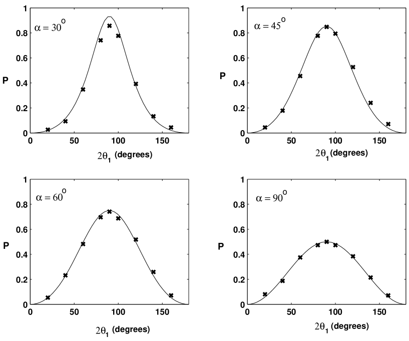
Figure 7:

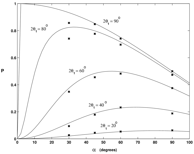
Figure 8:

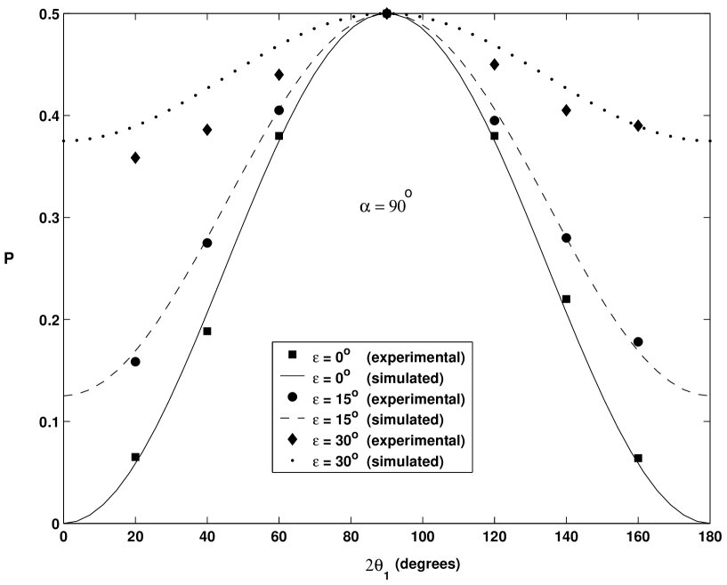
Figure 9:

References

- (1) R. Feynman, Int. j. Theor. phys. 21, 467 (1982).
- (2) C.H. Bennett, Int. J. Theor. Phys. 21 905 (1982).
- (3) D. Deutsch, Proc. R. Soc. London, Ser. A 400, 97 (1985)
- (4) S. Lloyd, Science 261, 1569 (1993).
- (5) P. W. Shor, SIAM Rev. 41, 303-332 (1999).
- (6) D. Deutsch and R. Jozsa, Proc. R. Soc. Lond. A 493, 553 (1992).
- (7) L.K. Grover, Phys. Rev. Lett. 79, 325 (1997).
- (8) J. Gruska ”Quantum Computing”, Mcgraw-Hill Limited, UK, 1999.
- (9) D. Bouwnmeester, A. Ekert, A. Zeilinger(Eds.), ”The Physics of Quantum Information”, Springer, Berlin, 2000.
- (10) M.A. Nielsen , I.L. Chuang, ”Quantum Computation and Quantum Information”. Cambridge University Press, Cambridge, U.K. 2000.
- (11) T. M . Cover and J. A. Thomas. Elements of Information Theory. John Wiely and Sons, Newyork, 1991.
- (12) I. L. chuang, L. M. K. Vanderspyen, X. Zhou, D. W. Leung, and S. Llyod, Nature (london), 393, 1443 (1998).
- (13) J.A. Jones and M. Mosca, J. Chem. Phys. 109, 1648 (1998).
- (14) I.L. Chuang, N. Gershenfeld, M. Kubinec, Phys. Rev. Lett. 80, 3408 (1998).
- (15) J.A. Jones, M. Mosca, and R. H. Hansen, Nature (London) 393, 344 (1998).
- (16) T. S. Mahesh, Kavita Dorai, Arvind, Anil Kumar, J. Mag. Res. 148, 95 (2001).
- (17) Neeraj Sinha, T. S. Mahesh, K.V. Ramanathan, and Anil Kumar, J. Chem. Phys. 114, (2001) 4415.
- (18) Ranabir Das, T.S. Mahesh, and Anil Kumar, J. Magn. Reson. 159 46 (2002).
- (19) Ranabir Das and Anil Kumar, Phys. Rev. A 68, 032304 (2003).
- (20) L.S.Philips, S. M. Barnett and D. T. Pegg, Phys. Rev. A. 58, 3259.
- (21) Zhang Shengyn,Feng Yuan, Sun Xiaoming, et al. Phys. Rev. A . 64, 062193
- (22) S. M. Barnett, Phys. Rev. A. 64, 030303.
- (23) A.Chefles, Phys. Rev. A. 64, 062305.
- (24) A.Chefles, Contemp. Phys. 41, 401 (2001).
- (25) C. W. Helsrom, Quantum Detection and Estimation Theory. (Acadamic Press, New York, 1976).
- (26) I. D. Ivanovic, Phys. Lett. A. 123, 257 (1987).
- (27) A. Peres, Phys. Lett. A. 128, 19 (1988).
- (28) A.Chefles and S. M. Barnett, Phys. Lett. A. 250, 223 (1998).
- (29) B. Huttner, A. Muller, J. D. Gautier, H.Zbinden, and N.Gisin Phys. Rev. A. 250, 223 (1998).
- (30) Miloslav Dusek and Vladimir Buzek, Phys. Rev. A. 66, 022112 (2002).
- (31) J. Fiurasek, M. Dusek, and R. Filip, Phys. Rev. Lett. 89, 190401 (2002).
- (32) J. Fiurasek and M. Dusek, Phys. Rev. A. 69, 032302 (2004).
- (33) J. P. Paz and A. Roncaglia, Phys. Rev. A. 68, 052316 (2003).
- (34) G. M. D’Ariano, P. Perinotti, M. F. Sacchi, Europhys. Lett. 65, 165 (2004).
- (35) M. A . Nielsen, I.L. Chuang, Phys. Rev. Lett.79, 321 (1997).
- (36) G. Vidal, L. Masanes, and J. I. Cirac, Phys. Rev. Lett. 88, 047905 (2002).
- (37) M. Hillery, V. Buzek, and M. Ziman, Phys. Rev. A. 65, 022301 (2002).
- (38) Jan Soubusta, Antonin Cernoch, Jaromir Fiurasek, and Miloslav Dusek, Phys. Rev. A. 69, 052321 (2004).
- (39) M. Dusek, M. Jahma, and N. Lutkenhaus, Phys. Rev. A. 62, 022306 (2000).
- (40) S.Hamieh, J. Phys. A: Math. Gen.. 37, L 59-L 61 (2004).
- (41) Yong Wook Cheong, Hyunjae Kim, and Hai-Woong Lee , Phys. Rev. A. 70, 032327 (2004).
- (42) Zhu - Liang Cao, Wei Song, quant-ph/0401054.
- (43) D. Collins, Phys. Rev. A 65, 052321 (2002).
- (44) Jaehyun Kim, Jae-Seung Lee, Taesoon Hwang, and Soonchil Lee , J. Mag. Res., 166, 35-38 (2004).
- (45) P.W. Shor, Phys. Rev. A 52, 2493 (1995).
- (46) D.G. Cory et al., Physica D 120, 82 (1998); J. Du etal., phys. rev. lett. 91, 100403 (2003).
- (47) Cory, D. G., Fahmy, A. F. and Havel, T. F., Ensemble quantum computing by NMR spectroscopy. Proc. Natl. Acad. Sci. USA, 94, 1634 (1997).
- (48) Gershenfeld, N. and Chuang, I. L., Bulk spin-resonance quantum computation. Science, 275, 350 (1997).
- (49) Knill, E., Chuang, I. L. and Laflammem R., Effective pure states for bulk quantum computation, Phys. Rev. A. 57, 3348 (1998).
- (50) Chuang, I. L., Gershenfeld, N, Kubines. M. G. and Leung, D. W., Bulk quantum computation with nuclear magnetic resonance, Proc. R. Soc. London, Ser. A, 454, 447-467 (1998).
- (51) Kavita Dorai, Arvind, Anil Kumar, Phys Rev A. 61, (2000) 042306.
- (52) T. S. Mahesh, Anil Kumar, Phys. Rev. A 64, 012307 (2001).
- (53) J. Du, H. Li, X. Xu, M. Shi, J. Wu, X. Zhou, and R. han, Phys. Rev. A 67, 042316 (2003).
- (54) R. R. Ernst, G.Bodenhausen, And A. Wokaun, Principles of Nuclear Magnetic Resonance in One and Two Dimensions, Oxford University Press 1987.