Minimal disturbance measurement for coherent states is non-Gaussian

Abstract

In standard coherent state teleportation with shared two-mode squeezed vacuum (TMSV) state there is a trade-off between the teleportation fidelity and the fidelity of estimation of the teleported state from results of the Bell measurement. Within the class of Gaussian operations this trade-off is optimal, i.e. there is not a Gaussian operation which would give for a given output fidelity a larger estimation fidelity. We show that this trade-off can be improved by up to $2.77\%$ if we use a suitable non-Gaussian operation. This operation can be implemented by the standard teleportation protocol in which the shared TMSV state is replaced with a suitable non-Gaussian entangled state. We also demonstrate that this operation can be used to enhance the transmission fidelity of a certain noisy channel.

I Introduction

In quantum mechanics there is not an operation which would give some information on an unknown quantum state without disturbing the state. This property of quantum mechanics is closely related to the no-cloning theorem Wootters_82 which forbids to perfectly duplicate an unknown quantum state. A question that can be risen in this context is which operation allowed by quantum mechanics approximates best this non-existing operation, i.e. which operation introduces for a given information gain the least possible disturbance. Naturally, this operation, conventionally denoted as minimal disturbance measurement (MDM), will in general depend on the set of input states, their a-priori distribution, and on the figures of merit used to quantify the information gain and the state disturbance. A convenient approach to the problem on finding the MDM was developed in Banaszek_01a . In this approach the classical information gained on the input state from a quantum operation is converted into the estimate of the input state and the information gain is then quantified by the average estimation fidelity $\bar{G}$, i.e. the fidelity $G$ between the estimate and the input state averaged over the distribution of the input states. On the other hand, the disturbance introduced by the operation into the input state is quantified by the average output fidelity $\bar{F}$, i.e. the fidelity $F$ between the input state and the state at the output of the operation averaged over the distribution of the input states. According to the laws of quantum mechanics for a given set of input states there exists a specific optimal trade-off between the fidelities $\bar{G}$ and $\bar{F}$ which cannot be overcome by any quantum operation. In terms of the fidelities $\bar{G}$ and $\bar{F}$ the MDM then can be defined as a quantum operation which saturates this optimal trade-off. First optimal fidelity trade-offs and the corresponding MDMs were derived in the context of finite-dimensional quantum systems and observables with discrete spectra. To be more specific, the MDMs were found analytically for a completely unknown Banaszek_01a and partially known Mista_05 $d$-level particle and numerically for $N$ identical copies of a completely unknown $2$-level particle (qubit) Banaszek_01b . In addition, the MDMs for a completely unknown as well as partially known qubit were demonstrated experimentally using a single-photon polarization qubit Sciarrino_05 . Besides being of fundamental interest MDM can be applied to increase the transmission fidelity of a certain lossy channel Ricci_05 .

Only recently the concept of MDM was also extended into the realm of systems with infinite-dimensional Hilbert spaces and observables with continuous spectrum-continuous variables (CVs). The attention has been paid to MDMs on Gaussian states, i.e. states represented by Gaussian Wigner function, realized by covariant Gaussian operations, i.e. operations preserving Gaussian states which are invariant under displacement transformations. These operations are advantageous since for coherent input states they posses state-independent output fidelity $F$ and estimation fidelity $G$ which can be conveniently used for characterization of state disturbance and information gain. Within the class of such operations optimal trade-off between the two fidelities as well as the corresponding MDM for the set of all coherent states with uniform a-priori distribution were derived in Andersen_05 ; Fiurasek_05 and realized experimentally in Andersen_05 . In addition, also this covariant Gaussian MDM was shown to be capable to increase transmission fidelity of some noisy channels Andersen_05 .

In this paper we address a natural question of whether the covariant Gaussian MDM for uniformly distributed coherent states can be improved. We answer this question in the affirmative. We show that the fidelity trade-off corresponding to this measurement can be increased by up to $2.77\%$ if we use a suitable non-Gaussian operation thus showing that MDM for coherent states is non-Gaussian. This MDM can be implemented using the standard continuous-variable (CV) teleportation protocol Vaidman_94 ; Braunstein_98 in which the participants share an appropriate non-Gaussian entangled state. Further, we demonstrate that our non-Gaussian MDM gives a higher transmission fidelity of a certain noisy channel in comparison with that achieved in Andersen_05 . As a by-product we also derive for the set of all coherent states with uniform a-priori distribution a lower bound for the optimal fidelity trade-off for any covariant quantum operation. The present paper is inspired by the recent result that fidelity of quantum cloning of coherent states can be increased by using a non-Gaussian entangled state Cerf_04 .

The paper is organized as follows. Section II deals with optimal Gaussian fidelity trade-off and corresponding MDM for uniformly distributed coherent states. In Section III we derive for this set of states a lower bound on optimal fidelity trade-off for any covariant quantum operation. Section IV is dedicated to implementation of a quantum operation saturating this bound and its application. Section V contains conclusions.

II Gaussian minimal disturbance measurement

The Gaussian MDM can be realized by at least three ways Andersen_05 encompassing the asymmetric cloning followed by a joint measurement, a linear-optical scheme with a feed forward or by the standard CV teleportation protocol proposed by Braunstein and Kimble (BK) Braunstein_98 and demonstrated experimentally in Furusawa_98 . With respect to what follows it is convenient to start with the implementation of the Gaussian MDM via BK teleportation protocol. Here we use an optical notation in which CV systems are realized by single modes of an optical field and the role of CVs is played by quadratures $x_{j}$ and $p_{k}$ ($[x_{j},p_{k}]=i\delta_{jk}$) of these modes.

In the BK protocol an unknown coherent state $|\alpha\rangle_{\rm in}$ of a mode “in” is teleported by sender Alice ($A$) to receiver Bob ($B$). In each run of the protocol, the state is chosen randomly with uniform distribution from the set of all coherent states. Initially, Alice and Bob share a two-mode squeezed vacuum (TMSV) state which is a Gaussian entangled state of two optical modes $A$ and $B$ described in the Fock basis as

$$|TMSV\rangle_{AB}=\sum_{n=0}^{\infty}\tilde{c}_{n}|n,n\rangle_{AB},\quad\tilde{c}_{n}=\sqrt{1-\lambda^{2}}\lambda^{n},$$ (1)

where $\lambda=\tanh r$ ($r$ is the squeezing parameter). Then, Alice performs the so called Bell measurement that consists of superimposing of modes “in” and $A$ on a balanced beam splitter and subsequent detection of the quadrature variables $x_{1}=(x_{\rm in}-x_{A})/\sqrt{2}$ and $p_{2}=(p_{\rm in}+p_{A})/\sqrt{2}$ at its outputs. She obtains classical results of the measurement $\bar{x}_{1}$ and $\bar{p}_{2}$ and sends them via classical channel to Bob who displaces his part of the shared state as $x_{B}\rightarrow x_{\rm out}=x_{B}+\sqrt{2}\bar{x}_{1}$ and $p_{B}\rightarrow p_{\rm out}=p_{B}+\sqrt{2}\bar{p}_{2}$. As a result, Bob’s output quadratures read as $x_{\rm out}=x_{\rm in}-\sqrt{2}e^{-r}x_{B}^{(0)}$ and $p_{\rm out}=p_{\rm in}+\sqrt{2}e^{-r}p_{A}^{(0)}$ Loock_00a , where $x_{i}^{(0)}$ and $p_{j}^{(0)}$ stand for initial vacuum quadratures. Since the squeezing $r$ is always finite in practice Bob has only an approximate replica $\rho_{\rm out}(\alpha)$ of the input state. Moreover, for the same reason Alice gains some information on the input state from results of the Bell measurement that can be converted into a classical estimate $\rho_{\rm est}(\alpha)$ of the input state by displacing a vacuum mode $E$ as $x_{E}^{(0)}\rightarrow x_{\rm est}=x_{E}^{(0)}+\sqrt{2}\bar{x}_{\rm 1}$ and $p_{E}^{(0)}\rightarrow p_{\rm est}=p_{E}^{(0)}+\sqrt{2}\bar{p}_{\rm 2}$. Hence she obtains $x_{\rm est}=x_{\rm in}+x_{E}^{(0)}-(e^{r}x_{A}^{(0)}+e^{-r}x_{B}^{(0)})/\sqrt{2}$ and $p_{\rm est}=p_{\rm in}+p_{E}^{(0)}+(e^{-r}p_{A}^{(0)}+e^{r}p_{B}^{(0)})/\sqrt{2}$. Quantifying now the resemblance of the states $\rho_{\rm out}(\alpha)$ and $\rho_{\rm est}(\alpha)$ to the input state $|\alpha\rangle$ by the output fidelity $F$ and the estimation fidelity $G$

$$F=\langle\alpha|\rho_{\rm out}(\alpha)|\alpha\rangle,\quad G=\langle\alpha|\rho_{\rm est}(\alpha)|\alpha\rangle,$$ (2)

one finds using the latter formulas that

$$F_{\rm BK}=\frac{1}{1+e^{-2r}},\quad G_{\rm BK}=\frac{1}{1+\cosh^{2}(r)}.$$ (3)

Expressing $\cosh^{2}(r)$ in terms of $F_{\rm BK}$ using the first formula and inserting this into the formula for $G_{\rm BK}$ we finally arrive at the following trade-off between the fidelities $F_{\rm BK}$ and $G_{\rm BK}$:

$$G_{\rm BK}=\frac{1}{1+\frac{1}{4F_{\rm BK}(1-F_{\rm BK})}}.$$ (4)

The obtained trade-off is depicted by dashed curve in Fig. 1. It is obvious from the figure that as one would expect the obtained fidelities exhibit complementary behavior, i.e. the larger is the estimation fidelity the smaller is the output fidelity and vice versa. Interestingly, it was shown in Andersen_05 ; Fiurasek_05 that if one restricts only to the covariant Gaussian operations, then the trade-off (4) is optimal. It means in other words that the standard BK teleportation protocol with shared TMSV state realizes (within the class of all covariant Gaussian operations) MDM for coherent states. In the following sections we demonstrate that the optimal Gaussian trade-off (4) can be improved by a suitable covariant non-Gaussian operation.

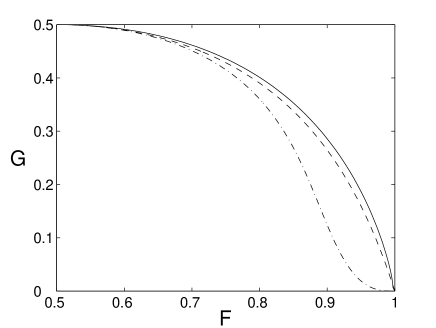
Figure 1: Trade-off between the otput fidelity $F$ and the estimation fidelity $G$ for the BK teleportation scheme with the shared optimized non-Gaussian state (solid curve), TMSV state (1) (dashed curve) and TMSV state de-gaussificated by local single photon subtraction from each mode (24) (dotted-dashed curve). See text for details.

III Optimal fidelity trade-off for coherent states

We start by a suitable mathematical formulation of the task on finding the optimal fidelity trade-off for CVs. For this purpose we use a general method developed in Mista_05 . We restrict our attention to coherent input states $|\alpha\rangle=D(\alpha)|0\rangle$, where $\alpha$ lies in the complex plane $\mathbb{C}$, which form the orbit of the Weyl-Heisenberg group. Here $|0\rangle$ is the vacuum state and the displacement operators $D(\alpha)=\mbox{exp}(\alpha a^{{\dagger}}-\alpha^{\ast}a)$, $\alpha\in\mathbb{C}$, where $a$ and $a^{{\dagger}}$ are the standard annihilation and creation operators satisfying boson commutation rule $[a,a^{{\dagger}}]=\openone$, comprise the irreducible unitary representation of this group. We also assume that the a-priori distribution of the input states coincides with the invariant measure on the group $d^{2}\alpha/\pi=d(\mbox{Re}\alpha)d(\mbox{Im}\alpha)/\pi$.

The standard BK teleportation protocol can be formally viewed as a trace-preserving quantum operation which is covariant, i.e. invariant under displacement transformations, and which can give as a measurement outcome any complex number $\beta$ ($\beta\equiv\bar{x}_{1}+i\bar{p}_{2}$ in the case of teleportation). Therefore, we will seek for the optimal fidelity trade-off on this set of quantum operations. To each outcome $\beta$ of such an operation we can assign a trace-decreasing completely positive (CP) map that can be represented by the following positive-semidefinite operator on the tensor product ${\mathcal{H}}_{\rm in}\otimes{\mathcal{H}}_{\rm out}$ of the input and output Hilbert spaces $\mathcal{H}_{\rm in}$ and $\mathcal{H}_{\rm out}$ Jamiolkowski_72

$$\chi(\beta)=[D_{\rm in}(\beta^{\ast})\otimes D_{\rm out}(\beta)]\chi_{0}[D_{\rm in}^{{\dagger}}(\beta^{\ast})\otimes D_{\rm out}^{{\dagger}}(\beta)],$$ (5)

where $\chi_{0}$ is a positive-semidefinite operator. For the measurement outcome $\beta$ the estimated state is $|\beta\rangle$ whereas the output state reads

$$\rho(\beta|\alpha)=\mathrm{Tr}_{\rm in}[\chi(\beta)(|\alpha\rangle_{\rm in}\langle\alpha|)^{\rm T}\otimes\openone_{\rm out}],$$ (6)

where $\openone_{\rm out}$ is the identity operator on $\mathcal{H}_{\rm out}$. Since the map $\chi(\beta)$ is trace-decreasing the output state (6) is not normalized to unity and its norm $P(\beta|\alpha)=\mathrm{Tr}_{\rm out}[\rho(\beta|\alpha)]$ is equal to the probability density of this outcome. The entire operation should be trace-preserving which imposes the following constraint:

$$\frac{1}{\pi}\int_{\mathbb{C}}\mathrm{Tr}_{\rm out}[\chi(\beta)]d^{2}\beta=\openone_{\rm in},$$ (7)

where $\int_{\mathbb{C}}$ denotes integration over the whole complex plane and $\openone_{\rm in}$ is the identity operator on $\mathcal{H}_{\rm in}$. For the input state $|\alpha\rangle$ the studied operation produces on average the output state and the estimated state in the form

$$\rho_{\rm out}(\alpha) = \frac{1}{\pi}\int_{\mathbb{C}}\rho(\beta|\alpha)d^{2}\beta,$$

$$\rho_{\rm est}(\alpha) = \frac{1}{\pi}\int_{\mathbb{C}}P(\beta|\alpha)|\beta\rangle\langle\beta|d^{2}\beta.$$ (8)

Making use of Eqs. (5), (6), (III) and the formula $D(-\beta)|\alpha\rangle=\mbox{exp}[i\mbox{Im}(\alpha\beta^{\ast})]|\alpha-\beta\rangle$ one finally finds the fidelities (2) to be

$$F=\mathrm{Tr}[\chi_{0}R_{F}],\qquad G=\mathrm{Tr}[\chi_{0}R_{G}],$$ (9)

where $R_{F}$ and $R_{G}$ are the positive-semidefinite Gaussian operators defined as

$$R_{F} = \frac{1}{\pi}\int_{\mathbb{C}}|\gamma^{\ast}\rangle_{\rm in}\langle\gamma^{\ast}|\otimes|\gamma\rangle_{\rm out}\langle\gamma|d^{2}\gamma,$$

$$R_{G} = \frac{1}{\pi}\int_{\mathbb{C}}e^{-|\gamma|^{2}}|\gamma\rangle_{\rm in}\langle\gamma|d^{2}\gamma\otimes\openone_{\rm out}.$$ (10)

The optimal trade-off between the fidelities $F$ and $G$ can be found by finding the maximum of the weighted sum

$$\mathcal{F}(p)=pF+(1-p)G$$ (11)

of these two fidelities Fiurasek_03 , where the parameter $p\in[0,1]$ controls the ratio between the information gained from the input state and the disturbance of this state. We can write $\mathcal{F}(p)=\mathrm{Tr}[\chi_{0}R(p)]$, where

$$R(p)=pR_{F}+(1-p)R_{G}.$$ (12)

Making use of the inequality $R(p)\leq\lambda_{\rm max}(p)(\openone_{\rm in}\otimes\openone_{\rm out})$, where $\lambda_{\rm max}(p)$ is the maximum eigenvalue of $R(p)$ and taking into account the condition $\mathrm{Tr}[\chi_{0}]=1$ which we obtain from the constraint (7) using the formula D'Ariano_04

$$\frac{1}{\pi}\int_{\mathbb{C}}D(\alpha)XD^{{\dagger}}(\alpha)d^{2}\alpha=\mathrm{Tr}[X]\openone$$ (13)

following from Schur’s lemma, one finds $\mathcal{F}(p)$ to be upper bounded as $\mathcal{F}(p)\leq\lambda_{\rm max}(p)$. Now, if we find a normalized eigenvector $|\chi_{\rm max}(p)\rangle$ of the operator $R(p)$ corresponding to the maximum eigenvalue $\lambda_{\rm max}(p)$, then the map (5) generated from any such $\chi_{0,{\rm max}}=|\chi_{\rm max}(p)\rangle\langle\chi_{\rm max}(p)|$ satisfies the trace-preservation condition (7) as follows from Eq. (13). Consequently, the map $\chi_{0,{\rm max}}$ is the optimal one that saturates optimal trade-off between $F$ and $G$.

The finding of the optimal fidelity trade-off thus boils down to the diagonalization of the operator $R(p)$ which acts on the direct product of two infinite-dimensional spaces. For this purpose it is convenient to express the operators $R_{F}$ and $R_{G}$ in the form:

$$R_{F} = \sum_{K=0}^{\infty}\frac{{K!}}{2^{K+1}}\sum_{n,m=0}^{K}\frac{|n\rangle_{\rm in}\langle K-m|\otimes|m\rangle_{\rm out}\langle K-n|}{\sqrt{{n!}{(K-m)!}{m!}{(K-n)!}}},$$

$$R_{G} = \sum_{n=0}^{\infty}\frac{1}{2^{n+1}}|n\rangle_{\rm in}\langle n|\otimes\openone_{\rm out},$$ (14)

which can be calculated from Eq. (III) using the formulas $|\gamma\rangle=e^{-|\gamma|^{2}/2}\sum_{n=0}^{\infty}(\gamma^{n}/\sqrt{n!})|n\rangle$ and $\int_{\mathbb{C}}e^{-s|\gamma|^{2}}\gamma^{n}{\gamma^{\ast}}^{m}d^{2}\gamma=(\pi{n!}/s^{n+1})\delta_{nm}$ (Re$s>0$). The present eigenvalue problem can be simplified, if we notice that both the operators (III) and therefore also the operator $R(p)$ commute with the operator of the photon number difference $N_{-}=n_{\rm in}-n_{\rm out}$, where $n_{i}=a_{i}^{{\dagger}}a_{i}$, $i={\rm in},{\rm out}$. Consequently, the total Hilbert space splits into the direct sum $\displaystyle{\mathcal{H}}_{\rm in}\otimes{\mathcal{H}}_{\rm out}=\mathop{\oplus}_{N=-\infty}^{+\infty}{\mathcal{H}}^{(N)}$ of the characteristic subspaces ${\mathcal{H}}^{(N)}$ of the operator $N_{-}$ corresponding to the eigenvalues $N=-\infty,\ldots,+\infty$. The infinite-dimensional subspaces ${\mathcal{H}}^{(+L)}$ (${\mathcal{H}}^{(-L)}$), $L=0,1,\ldots$ are spanned by the basis vectors $\{|n+L,n\rangle_{\rm in,out},n=0,1,\ldots\}$ ($\{|n,n+L\rangle_{\rm in,out},n=0,1,\ldots\}$). Hence, it remains to diagonalize the operator $R(p)$ in the subspaces ${\mathcal{H}}^{(\pm L)}$ where it is represented by infinite-dimensional matrices $R^{(\pm L)}(p)=pR_{F}^{(\pm L)}+(1-p)R_{G}^{(\pm L)}$, where

$$\left(R_{F}^{(\pm L)}\right)_{nm} = \frac{\sqrt{\left({n+m+L\atop n}\right)\left({n+m+L\atop m}\right)}}{2^{L+n+m+1}},$$

$$\left(R_{G}^{(+L)}\right)_{nm} = \frac{\delta_{nm}}{2^{n+L+1}},\quad\left(R_{G}^{(-L)}\right)_{nm}=\frac{\delta_{nm}}{2^{n+1}},$$

where $n,m=0,1,\ldots$.

We have accomplished this task numerically and the obtained fidelity trade-off is depicted by the solid curve in Fig. 1. The figure clearly demonstrates that this trade-off beats the optimal Gaussian trade-off (4) (dashed curve). In order to see the degree of improvement better we have plotted by a solid curve in Fig. 2 the dependence of difference $\Delta G=G-G_{\rm BK}$ between the estimation fidelity $G$ in the improved trade-off and the estimation fidelity $G_{\rm BK}$ in the optimal Gaussian trade-off on the output fidelity $F$. Numerical analysis reveals that, for instance, $\Delta G\approx 1.04\%$ is achieved for $F\approx 0.794$ and the maximum improvement of $\Delta G\approx 2.77\%$ is attained for $F=F_{\rm max}\approx 0.963$.

It should be stressed that we have in fact found a lower bound on the optimal trade-off because we have approximated each original infinite-dimensional matrix $R^{(\pm L)}(p)$ by its $\mathcal{N}$-dimensional submatrix $R_{\mathcal{N}}^{(+L)}(p)$ ($R_{\mathcal{N}}^{(-L)}(p)$) on the $\mathcal{N}$-dimensional subspace ${\mathcal{H}}_{\mathcal{N}}^{(+L)}$ (${\mathcal{H}}_{\mathcal{N}}^{(-L)}$) spanned by the basis vectors $\{|n+L,n\rangle_{\rm in,out},n=0,1,\ldots,\mathcal{N}-1\}$ ($\{|n,n+L\rangle_{\rm in,out},n=0,1,\ldots,\mathcal{N}-1\}$). This follows from the inequality

$$\langle\psi_{\mathcal{N}}|R_{\mathcal{N}}^{(\pm L)}(p)|\psi_{\mathcal{N}}\rangle=\langle\psi_{\mathcal{N}}|R(p)|\psi_{\mathcal{N}}\rangle\leq\lambda_{\rm max}(p),$$ (16)

which holds for any $|\psi_{\mathcal{N}}\rangle\in{\mathcal{H}}_{\mathcal{N}}^{(\pm L)}$. Therefore, because we only calculated the eigenvector corresponding to maximum eigenvalue of matrices $R_{\mathcal{N}}^{(\pm L)}(p)$ (here we took $\mathcal{N}=500$ and $L\leq 30$), the optimal trade-off can be slightly larger than that given by the solid curve in Fig. 1.

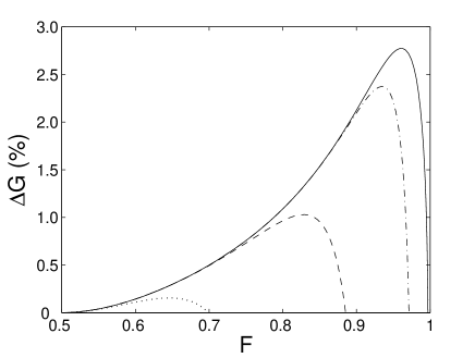
Figure 2: Difference $\Delta G=G-G_{\rm BK}$ between the estimation fidelity $G$ in the improved fidelity trade-off and the estimation fidelity $G_{\rm BK}$ in the optimal Gaussian trade-off versus the output fidelity $F$ for $\mathcal{N}=4$ (dotted curve), $\mathcal{N}=12$ (dashed curve), $\mathcal{N}=50$ (dotted-dashed curve), $\mathcal{N}=500$ (solid curve). See text for details.

IV Implementation

The above analysis shows that the optimal eigenvector $|\chi_{\rm max}(p)\rangle$ lies in one of the subspaces ${\mathcal{H}}^{(\pm L)}$. We have a strong numerical evidence that it lies in the subspace corresponding to $L=0$, i.e. it has the structure

$$|\chi_{\rm max}(p)\rangle=\sum_{n=0}^{\infty}c_{n}|n,n\rangle_{AB},$$ (17)

and, in addition, the probability amplitudes $c_{n}$ comprising the dominant eigenvector of the matrix $R^{(0)}(p)$ are nonnegative. The latter statement follows immediately from positivity of elements of the matrix $R(p)$. The optimal CP map (5) corresponding to the vector (17) can be implemented by the BK teleportation scheme in which the TMSV state (1) is replaced by this vector. This can be shown if we describe the BK teleportation by the transfer operator method Hofmann_01 . In this formalism, the action of the BK teleporter with shared entangled state $\sum_{n=0}^{\infty}c_{n}|n,n\rangle_{AB}$ is described by the set of transfer operators $\{T(\beta)=D(\beta)T(0)D^{{\dagger}}(\beta)\}_{\beta\in\mathbb{C}}$, where $T(0)=\sum_{n=0}^{\infty}c_{n}|n\rangle\langle n|$. If the input state is $|\alpha\rangle$ and the Bell measurement gives the outcome $\beta=\bar{x}_{1}+i\bar{p}_{2}$ the output state reads as $|\psi_{\rm out}(\beta|\alpha)\rangle=T(\beta)|\alpha\rangle$. The state $|\chi_{0}\rangle$ forming the positive-semidefinite operator $\chi_{0}$ describing the considered teleportation protocol then can be calculated by acting with the operator $T(0)$ on one part of maximally entangled state $\sum_{n=0}^{\infty}|n,n\rangle_{AB}$ Jamiolkowski_72 . This finally gives the state $|\chi_{0}\rangle=T_{B}(0)\sum_{n=0}^{\infty}|n,n\rangle_{AB}$, which coincides exactly with the state (17).

Likewise, we can implement the quantum operation which saturates the fidelity trade-off depicted by the solid curve in Fig. 1. For this purpose, we need to prepare the entangled state

$$\sum_{n=0}^{\mathcal{N}-1}c_{n}|n,n\rangle_{AB},$$ (18)

where nonnegative probability amplitudes $c_{n}$ form the dominant eigenvector of the matrix $R_{\mathcal{N}}^{(0)}(p)$. Apparently, the improvement $\Delta G$ which can be achieved when using the state (18) will vary with the dimension $\mathcal{N}$ of the truncated space ${\mathcal{H}}_{\mathcal{N}}^{(0)}$. This dependence is depicted in Fig. 2. We see from the figure that the maximum improvement increases and moves towards larger values of $F$ as $\mathcal{N}$ grows. It is also seen from the figure that in order to achieve $\Delta G\approx 1\%$ one needs at least $\mathcal{N}\geq 12$. For values of $\mathcal{N}$ where the improvement $\Delta G$ achieves at least a few tenths of percent one can calculate the probability amplitudes $c_{n}$ of the state (18) only numerically. In order to demonstrate the difference between the state (18) and the optimal Gaussian state (1) we display in Fig. 3 the difference $\Delta c_{n}=c_{n}-\tilde{c}_{n}$ of the Schmidt coefficient $c_{n}$ of the state (18) with $\mathcal{N}=500$ and the Schmidt coefficient $\tilde{c}_{n}$ of the TMSV state (1) for $F=F_{\rm max}\approx 0.963$ versus the photon number. The state (18) can be prepared, at least in principle, using the probabilistic scheme for preparation of an arbitrary two-mode state with finite Fock state expansion based on linear optics Kok_02 .

The specific feature of the optimal state (17) is that it possesses perfect correlations in photon number as the TMSV state (1). However, there is a sharp difference between the two states, because in contrast with the latter state the former one is non-Gaussian. To show this assume on the contrary that the state (17) is a Gaussian state of two modes $A$ and $B$. Such a state is completely characterized by the first moments $\langle\xi_{k}\rangle=\langle\chi_{\rm max}(p)|\xi_{k}|\chi_{\rm max}(p)\rangle$, where $\xi=(x_{A},p_{A},x_{B},p_{B})^{\rm T}$, and by the variance matrix $V$ with elements $V_{kl}=\langle\{\Delta\xi_{k},\Delta\xi_{l}\}\rangle$, where $\Delta\xi_{k}=\xi_{k}-\langle\xi_{k}\rangle$ and $\{A,B\}\equiv(1/2)(AB+BA)$. As $\langle\xi\rangle=0$ for the state (17), it is completely described just by the variance matrix which reads as

$$V=\left(\begin{array}[]{cccc}a&0&c&0\\ 0&a&0&-c\\ c&0&a&0\\ 0&-c&0&a\\ \end{array}\right),$$ (23)

where $a=\sum_{n=0}^{\infty}nc_{n}^{2}+1/2$ and $c=\sum_{n=0}^{\infty}(n+1)c_{n}c_{n+1}\geq 0$. Taking into account the purity of the state, which imposes the constraint $\sqrt{\mbox{det}V}=a^{2}-c^{2}=1/4$ Trifonov_97 we see that such a state would be a TMSV state (1) with $\lambda=\sqrt{(a-1/2)/(a+1/2)}$ which does not beat the trade-off of the BK scheme and thus we arrive to a contradiction. Therefore, the state (17) is inevitably non-Gaussian. Thus we have found a non-Gaussian operation which possesses a better trade-off between output and estimation fidelities than any covariant Gaussian operation which implies that MDM for a completely unknown coherent state is non-Gaussian.

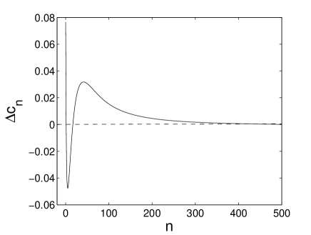
Figure 3: Dependence of the difference $\Delta c_{n}=c_{n}-\tilde{c}_{n}$ of the Schmidt coefficient $c_{n}$ of the entangled state (18) with $\mathcal{N}=500$ and the Schmidt coefficient $\tilde{c}_{n}$ of the TMSV state (1) for $F=F_{\rm max}\approx 0.963$ on the photon number.

It can be interesting to compare the fidelity trade-off derived by us with the trade-off that would be obtained when teleporting with the state produced by local single photon subtraction from each mode of a TMSV state. Originally investigated in the context of increase of teleportation fidelity via local operations and classical communication Opatrny_00 ; Cochrane_02 ; Olivares_03 the state was also shown to be suitable for loophole-free Bell test based on homodyne detection Nha_04 ; Garcia-Patron_04 ; Olivares_04 ; Garcia-Patron_05 . The reason for studying the state here is twofold. First, the state is a non-Gaussian state of the form Cochrane_02 ; Garcia-Patron_05

$$\sqrt{\frac{(1-T^{2}\lambda^{2})^{3}}{1+T^{2}\lambda^{2}}}\sum_{n=0}^{\infty}(n+1)(T\lambda)^{n}|n,n\rangle_{AB},$$ (24)

where $T$ is a transmittance of an unbalanced beam splitter used for photon subtraction and therefore it possesses perfect correlations in photon number as the optimal state (17). Second, the subtraction of a single photon was already demonstrated experimentally for a single-mode squeezed vacuum state Wenger_04 . Making use of the formulas

$$F=\sum_{m,n=0}^{\infty}{m+n\choose n}\frac{c_{m}^{\ast}c_{n}}{2^{m+n+1}},\quad G=\sum_{n=0}^{\infty}\frac{|c_{n}|^{2}}{2^{n+1}}$$

for the teleportation and estimation fidelities in the BK teleportation with the shared state (17) we can find using Eq. (24) the teleportation fidelity to be Olivares_03

$$F_{\rm s}=\frac{(1+T\lambda)^{3}(2-2T\lambda+T^{2}\lambda^{2})}{4(1+T^{2}\lambda^{2})},$$

while the estimation fidelity reads as

$$G_{\rm s}=2\left(\frac{2+T^{2}\lambda^{2}}{1+T^{2}\lambda^{2}}\right)\left(\frac{1-T^{2}\lambda^{2}}{2-T^{2}\lambda^{2}}\right)^{3}.$$

The trade-off between the fidelities $F_{\rm s}$ and $G_{\rm s}$ is depicted by the dotted-dashed curve in Fig. 1. The figure clearly reveals that the trade-off is even worse than the optimal Gaussian trade-off (4). Thus while the single photon subtraction can be a useful method for distillation of the CV entanglement and test of Bell inequalities it is not suitable for preparation of a non-Gaussian entangled state which would improve fidelity trade-off in teleportation of coherent states.

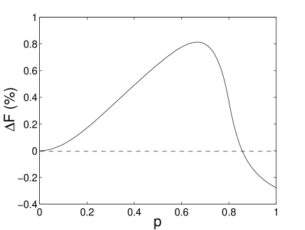
Figure 4: Dependence of the difference $\Delta F=\mathcal{F}-\mathcal{F}_{\rm BK}$ of the transmission fidelity $\mathcal{F}=pF+(1-p)G$ for the non-Gaussian operation and the transmission fidelity $\mathcal{F}_{\rm BK}=pF_{\rm BK}+(1-p)G_{\rm BK}$ maximized with respect to the squeezing parameter $r$ on the transmission probability $p$. See text for details.

The non-Gaussian operation realized by the BK teleportation protocol with shared non-Gaussian state (18) can be applied to enhance the transmission fidelity of a certain noisy channel. The channel in question transmits perfectly with probability $p$ the input coherent state while with probability $1-p$ the state is completely absorbed by the channel. For the set of all coherent states with uniform a-priori distribution the channel possesses the average transmission fidelity equal to $\mathcal{F}_{\rm av}(p)=p$. In Andersen_05 it was demonstrated that for $0<p<4/5$ the transmission fidelity can be improved by using the Gaussian MDM in front of the channel while for $p\geq 4/5$ it is better to entirely use the channel. Using the BK teleportation protocol to realize the MDM the improved scheme works as follows. Instead of sending directly the input coherent state through the channel one sends through it one part of the TMSV state (1). In the next step the other part of thus obtained state is used for teleportation of the input coherent state. The transmission fidelity for this scheme is given by the formula $\mathcal{F}_{\rm BK}(p)=pF_{\rm BK}+(1-p)G_{\rm BK}$, where the fidelities $F_{\rm BK}$ and $G_{\rm BK}$ are given in Eq. (3). By maximizing the transmission fidelity $\mathcal{F}_{\rm BK}(p)$ with respect to the squeezing parameter $r$ we can reach optimal performance of the scheme when in the interval $0<p<4/5$ $\mathcal{F}_{\rm BK}(p)>\mathcal{F}_{\rm av}(p)$ Andersen_05 . Interestingly, the transmission fidelity of the channel can be further improved provided that we use in the BK teleportation the non-Gaussian entangled state (18) ($\mathcal{N}=500$) as a quantum channel. This scheme must be inevitably optimal since within the class of all covariant operations it is designed in such a way that it maximizes the quantity (11) which is in fact the transmission fidelity of the considered channel. The dependence of the improvement $\Delta F(p)=\mathcal{F}(p)-\mathcal{F}_{\rm BK}(p)$ on the probability $p$ for our scheme is depicted in Fig. 4. The figure reveals that for $0<p\lesssim 0.85$ the scheme really allows to slightly improve the transmission fidelity the maximum improvement of $\Delta F\approx 0.81\%$ being achieved for $p=0.67$. In the region of $p\gtrsim 0.85$ $\Delta F$ attains negative values which is a numerical artefact caused by the truncation of the infinite-dimensional matrix $R^{(0)}(p)$ to the finite-dimensional matrix $R_{\mathcal{N}}^{(0)}(p)$. Therefore, in order to achieve $\Delta F>0$ also for some $p\gtrsim 0.85$ we would need to use in teleportation the state (18) with $\mathcal{N}>500$. If this is not possible then for $p\gtrsim 0.85$ it is better to send directly the input coherent state through the channel rather than to use our non-Gaussian operation. Thus we have illustrated also practical utility of the studied non-Gaussian operation for increase of the transmission fidelity of a specific quantum channel.

V Conclusions

In conclusion, we have shown that there exists a covariant non-Gaussian quantum operation which gives for a completely unknown coherent state a better trade-off between the output fidelity and the estimation fidelity than any covariant Gaussian operation. This means that the covariant MDM for a completely unknown coherent state is non-Gaussian. The non-Gaussian operation can be implemented by the standard BK teleportation protocol with a suitable non-Gaussian entangled state as a quantum channel and can be utilized to enhance the transmission fidelity of a certain channel. As a by-product we also derived a lower bound for the optimal fidelity trade-off for a completely unknown coherent state within the class all covariant quantum operations. Our result thus clearly illustrates that one can extract more information on an unknown coherent state while preserving the degree of disturbance introduced into it by this procedure by using a suitable non-Gaussian operation.

- (1) W. K. Wootters and W. H. Zurek, Nature (London) 299, 802 (1982).
- (2) K. Banaszek, Phys. Rev. Lett. 86, 1366 (2001).
- (3) L. Mišta, Jr., J. Fiurášek, and R. Filip, Phys. Rev. A 72, 012311 (2005).
- (4) K. Banaszek and I. Devetak, Phys. Rev. A 64, 052307 (2001).
- (5) F. Sciarrino, M. Ricci, F. De Martini, R. Filip, and L. Mišta, Jr., e-print quant-ph/0510097.
- (6) M. Ricci, F. Sciarrino, N. J. Cerf, R. Filip, J. Fiurášek, and F. De Martini, Phys. Rev. Lett. 95, 090504 (2005).
- (7) U. L. Andersen, M. Sabuncu, R. Filip, and G. Leuchs, e-print quant-ph/0510195.
- (8) J. Fiurášek (private communication).
- (9) L. Vaidman, Phys. Rev. A 49, 1473 (1994).
- (10) S. L. Braunstein and H. J. Kimble, Phys. Rev. Lett. 80, 869 (1998).
- (11) N. J. Cerf, O. Krüger, P. Navez, R. F. Werner, and M. M. Wolf, Phys. Rev. Lett. 95, 070501 (2005).
- (12) A. Furusawa, J. L. Sørensen, S. L. Braunstein, C. A. Fuchs, H. J. Kimble, and E. S. Polzik, Science 282, 706 (1998); W. P. Bowen, N. Treps, B. C. Buchler, R. Schnabel, T. C. Ralph, H.-A. Bachor, T. Symul, and P. K. Lam, Phys. Rev. A 67, 032302 (2003); T. C. Zhang, K. W. Goh, C. W. Chou, P. Lodahl, and H. J. Kimble, Phys. Rev. A 67, 033802 (2003).
- (13) P. van Loock and S. L. Braunstein, Phys. Rev. Lett. 84, 3482 (2000).
- (14) A. Jamiolkowski, Rep. Math. Phys. 3, 275 (1972); M.-D. Choi, Linear Algebr. Appl. 10, 285 (1975).
- (15) J. Fiurášek, Phys. Rev. A 67, 052314 (2003); J. Fiurášek, R. Filip, and N. J. Cerf, Quant. Inf. Comp. 5, 583 (2005).
- (16) G. M. D’Ariano, P. Perinotti, and M. F. Sacchi, J. Opt. B: Quantum Semiclassical Opt. 6, 487 (2004).
- (17) H. Hofmann, T. Ide, T. Kobayashi, and A. Furusawa, Phys. Rev. A 64, 040301(R) (2001).
- (18) P. Kok, H. Lee, and J. P. Dowling, Phys. Rev. A 65, 052104 (2002); J. Fiurášek, S. Massar, and N. J. Cerf, Phys. Rev. A 68, 042325 (2003).
- (19) D. A. Trifonov, J. Phys. A: Math. Gen. 30, 5941 (1997).
- (20) T. Opatrný, G. Kurizki, and D.-G. Welsch, Phys. Rev. A 61, 032302 (2000).
- (21) P. T. Cochrane, T. C. Ralph, and G. J. Milburn, Phys. Rev. A 65, 062306 (2002).
- (22) S. Olivares, M. G. A. Paris, and R. Bonifacio, Phys. Rev. A 67, 032314 (2003).
- (23) H. Nha and H. J. Carmichael, Phys. Rev. Lett. 93, 020401 (2004).
- (24) R. García-Patrón, J. Fiurášek, N. J. Cerf, J. Wenger, R. Tualle-Brouri, and P. Grangier, Phys. Rev. Lett. 93, 130409 (2004).
- (25) S. Olivares and M. G. A. Paris, Phys. Rev. A 70, 032112 (2004).
- (26) R. García-Patrón, J. Fiurášek, and N. J. Cerf, Phys. Rev. A 71, 022105 (2005).
- (27) J. Wenger, R. Tualle-Brouri, and P. Grangier, Phys. Rev. Lett. 92, 153601 (2004).