Lyapunov Generation of Entanglement and the Correspondence Principle

Abstract

We show how a classically vanishing interaction generates entanglement between two initially nonentangled particles, without affecting their classical dynamics. For chaotic dynamics, the rate of entanglement is shown to saturate at the Lyapunov exponent of the classical dynamics as the interaction strength increases. In the saturation regime, the one-particle Wigner function follows classical dynamics better and better as one goes deeper and deeper in the semiclassical limit. This demonstrates that quantum-classical correspondence at the microscopic level requires neither high temperatures, nor coupling to a large number of external degrees of freedom.

In the decades since its inception, no observed phenomenon, nor experimental result ever contradicted quantum theory. Yet, the world surrounding us, though being made out of quantum mechanical building blocks, behaves classically most of the time. This suggests that, one way or another, classical physics emerges out of quantum mechanics. Today’s common understanding of this quantum-classical correspondence is based on the realization that no finite-sized system is ever fully isolated. It is then hoped that a large regime of parameters exists where the coupling of the system to external degrees of freedom (to be called the environment from now on) destroys quantum interferences without modifying the system’s classical dynamics. Indeed, such a coupling usually induces loss of coherence on a time scale much shorter than it relaxes the system Joos03 ; Zurek03 .

The standard approach to decoherence starts from a master equation valid in the regime of weak system-environment coupling Joos03 ; Zurek03 . The master equation determines the time-evolution of the system’s Wigner function $W({\bf p},{\bf q})=(2\pi\hbar)^{-d}\int{\rm d}{\bf x}\exp[i{\bf p}{\bf x}]\rho({\bf q}+{\bf x}/2,{\bf q}-{\bf x}/2)$ ($\rho$ is the system’s density matrix) as

$$\partial_{t}W = \Big{\{}H,W\Big{\}}+\sum_{n\geq 1}\frac{(i\hbar)^{2n}}{2^{2n}(2n+1)!}\partial_{q}^{2n+1}V\partial_{p}^{2n+1}W$$ (1)

$$+2\gamma\partial_{p}(pW)+D\partial^{2}_{p}W.$$

The first term on the right-hand side of Eq. (1) is the classical Poisson bracket. The second term, written here for the case of a momentum-independent potential $V({\bf q})$, exists already in closed systems and generates quantum corrections to the dynamical evolution of $W$. This term starts to become comparable to the Poisson bracket at the Ehrenfest time $\tau_{\rm E}=\lambda^{-1}\ln N$, where $\lambda$ is the Lyapunov exponent of the classical dynamics, and $N$ the size of the system’s Hilbert space. The two terms on the second line of Eq. (1) are induced by the coupling to the environment. In the limit of weak coupling, $\gamma\rightarrow 0$, but finite diffusion constant, $D\propto\gamma T={\rm Cst}$, the friction term vanishes, leaving the classical dynamics unaffected. This requires to consider the high temperature limit. Simultaneously, for large enough $D$, the momentum diffusion term induces enough noise so as to kill the quantum corrections before they become important. The time-evolution of $W$ is then solely governed by the classical Poisson bracket, that is to say, classical dynamics emerges out of quantum mechanics. Refs. Habib ; Davidovich provided for a numerical illustration of this scenario.

Our motivations in this article are as follows. First, it is unclear how generic the above scenario is, since it is based on a master equation derived under restrictive assumptions, for instance on the environment, the dimensionality of the system or the strength of the coupling between system and environment Joos03 ; Zurek03 . Also, it formally requires to consider infinite temperatures. Moreover, and with the specific exception of the kicked harmonic oscillator investigated in Ref. Davidovich , there is not much analytical understanding of the decoherence process in generic dynamical systems, i.e. except for the regular case, master equations are usually integrated numerically. Second, claims have been made of an entropy production due to the coupling to environmental degrees of freedom governed by the system’s exponent $\lambda$ Zurek03 ; entropy , without clear analytical derivation, nor strong numerical evidence caveat1 . A Lyapunov decay of the fidelity has recently been analytically predicted Jal01 and numerically observed Jac01 , however, decoherence and fidelity are two different things, especially in the generic situation where the system and environment Hamiltonians do not commute with the coupling Hamiltonian Jac04 ; Cuc03 .

We revisit these issues and consider two interacting quantized dynamical systems. Entanglement generation between two particles has already been considered in Refs. furuya98 ; miller99 ; tanaka02 ; Jac04 ; Prosen05 . All results to date are consistent with the scenario proposed in Ref. Jac04 , according to which bipartite entanglement results from two contributions: (i) a quantum-mechanical one, which depends on the coupling strength between the two systems, and (ii) a dynamical one, which, in chaotic systems, is determined by the total system’s spectrum of Lyapunov exponents. The entanglement generation rate is given by the weakest of the coupling strength and the Lyapunov exponent. It has to be pointed out that this picture holds in the regime of classically weak but quantum-mechanically strong coupling (this will be made quantitative below). For regular systems, entanglement generation is slower than for chaotic ones, typically power-law in time Jac04 ; Prosen05 .

The purpose of this letter is threefold. First, we address the problem of decoherence and bipartite entanglement from a microscopic point of view, i.e. without relying on effective differential equations. This allows for a clear identification of the regime of validity of our theory. Second, we give strong numerical evidences for the existence of a Lyapunov regime of entanglement in bipartite systems (the numerical evidences presented in Ref. miller99 were challenged in Ref. tanaka02 ). Third, we discuss our results from the point of view of the quantum-classical correspondence, and present numerical phase-space dynamics results showing that this correspondence is fully achieved in the regime of Lyapunov entanglement. This is, we believe, the first clear microscopic illustration of the quantum-classical correspondence in a generic chaotic system.

As our starting point, we consider the Hamiltonian

$${\cal H}=H_{1}\otimes I_{2}+I_{1}\otimes H_{2}+\hbar\;{\cal U}.$$ (2)

We take chaotic one-particle Hamiltonians $H_{1,2}$. We specify that the interaction potential ${\cal U}$ is smooth, varying over a distance much larger than the particles’ de Broglie wavelength $\sigma$, and that it depends only on the distance between the particles. Planck’s constant in front of ${\cal U}$ in Eq. (2) makes it explicit that we consider a semiclassically vanishing two-particle interaction, i.e. the classical Hamiltonian corresponding to Eq. (2) does not couple the two particles. Our goal is to calculate the purity ${\cal P}(t)={\rm Tr}_{1}[\rho_{1}^{2}(t)]$ of the reduced density matrix $\rho_{1}(t)={\rm Tr}_{2}\rho(t)$. In the situation we consider of a unitary two-particle dynamics acting on an initially pure two-particle state, ${\cal P}(t)$ is a good measure of entanglement, which varies between 1 for product states and 0 for maximally entangled states. The calculation proceeds along the lines of Ref. Jac04 , and here we only sketch it. A similar semiclassical approach has been applied to a stochastic Schrödinger equation in Ref. Kolovsky .

In the initial two-particle product state we take, each particle is in a Gaussian wavepacket $\psi_{1,2}({\bf y})=(\pi\sigma^{2})^{-d/4}\exp[i{\bf p}_{1,2}\cdot({\bf y}-{\bf r}_{1,2})/\hbar-|{\bf y}-{\bf r}_{1,2}|^{2}/2\sigma^{2}]$. The two-particle density matrix evolves according to $\rho(t)=\exp[-i{\cal H}t/\hbar]|\psi_{1};\psi_{2}\rangle\langle\psi_{1};\psi_{2}|\exp[i{\cal H}t/\hbar]$ This time-evolution is evaluated semiclassically by means of the semiclassical two-particle propagator

$$\langle{\bf x}_{1},{\bf x}_{2}|e^{-i{\cal H}t/\hbar}|{\bf y}_{1},{\bf y}_{2}\rangle=\sum_{s,s^{\prime}}C_{s,s^{\prime}}^{1/2}e^{i[(S_{s}+S_{s^{\prime}})/\hbar+{\cal S}_{s,s^{\prime}}]}$$ (3)

which is expressed as a sum over pairs of classical trajectories, labelled $s$ and $s^{\prime}$, respectively connecting ${\bf y}_{1}$ to ${\bf x}_{1}$ and ${\bf y}_{2}$ to ${\bf x}_{2}$ in the time $t$. Because of our assumption of a semiclassically vanishing coupling, these classical trajectories are determined by the one-particle Hamiltonians. Each pair of such trajectories gives a contribution weighted by $C_{s,s^{\prime}}$, the inverse of the determinant of the stability matrix on $s$ and $s^{\prime}$, and oscillating with one-particle (denoted by $S_{s}$ and $S_{s^{\prime}}$) and two-particle (denoted by ${\cal S}_{s,s^{\prime}}=\int_{0}^{t}dt^{\prime}{\cal U}[{\bf q}^{(1)}_{s}(t^{\prime}),{\bf q}^{(2)}_{s^{\prime}}(t^{\prime})]$) action integrals accumulated by the first and second particles along $s$ and $s^{\prime}$ respectively. In the regime of semiclassically vanishing coupling we consider, the one-particle actions generate much faster oscillations than their two-particle counterpart. Accordingly, our approach relies on stationary phase conditions imposed on the one-particle actions. In Eq. (3), Maslov indices have been omitted since they drop out of the calculation.

To leading order in $\hbar_{\rm eff}=2\pi/N_{1,2}$ ($N_{i}$ is the size of the $i^{\rm th}$ system’s Hilbert space), our semiclassical calculation gives the time-evolution of the purity as

$${\cal P}(t) \simeq \sum_{i=1,2}\alpha_{i}\Theta(t>\tau_{i})\exp[-\lambda_{i}t]+\exp[-2\Gamma t]$$ (4)

$$+\Theta(t>\tau^{(1)}_{\rm E})N_{1}^{-1}+\Theta(t>\tau^{(2)}_{\rm E})N_{2}^{-1}.$$

The first, classical term decays with the Lyapunov exponents $\lambda_{1,2}$ caveat2 . It does not exist at short times, $t<\tau_{i}=\lambda_{i}^{-1}\ln[\lambda_{i}/\sigma^{2}G_{i}]$, ($G_{i}=\int{\rm d}t^{\prime}\langle\partial_{q}^{(i)}{\cal U}[{\bf q}^{(1)}_{s}(0),{\bf q}^{(2)}_{s^{\prime}}(0)]\;\partial_{q}^{(i)}{\cal U}[{\bf q}^{(1)}_{s}(t^{\prime}),{\bf q}^{(2)}_{s^{\prime}}(t^{\prime})]\rangle$), and has prefactors $\alpha_{i}={\cal O}(1)$. The second term is the standard, interaction-dependent quantum term with $\Gamma=\int_{0}^{t}{\rm d}t^{\prime}\langle{\cal U}[{\bf q}^{(1)}_{s}(0),{\bf q}^{(2)}_{s^{\prime}}(0)]\;{\cal U}[{\bf q}^{(1)}_{s}(t^{\prime}),{\bf q}^{(2)}_{s^{\prime}}(t^{\prime})]\rangle$, assuming a fast decay of correlations. Being given by the correlator of a classical potential evaluated along classical trajectories, $\Gamma$ does not depend on $\hbar$. Finally, the third and fourth, saturation terms in Eq. (4) set in after $\tau_{\rm E}^{(i)}=\lambda^{-1}_{i}\ln N_{i}$.

The validity of our approach is given by $\delta_{2}\leq\Gamma\leq B_{2}$, where $B_{2}$ and $\delta_{2}=B_{2}/(N_{1}N_{2})$ are the two-particle bandwidth and level spacing respectively Jac01 . In this range, ${\cal U}$ is quantum-mechanically strong as individual levels are broadened beyond their average spacing, but classically weak, as $B_{2}$ is unaffected by ${\cal U}$ Jal01 ; Jac01 . We note that our semiclassical approach preserves the properties of the density matrix ${\rm Tr}_{1}[\rho_{1}(t)]=1$, $\rho_{1}=\rho_{1}^{\dagger}$, as well as the symmetry ${\rm Tr}_{1}[\rho_{1}^{2}(t)]={\rm Tr}_{2}[\rho_{2}^{2}(t)]$.

Eq. (4) expresses the decay of ${\cal P}(t)$ as a sum over dynamical, purely classical contributions, and quantal ones, depending on the interaction strength. Because the decaying terms are exponential and have prefactors of order unity, one has for $t>\tau^{(1,2)}_{\rm E},\tau_{1,2}$

$${\cal P}(t)\simeq\exp[-{\rm min}(\lambda_{1},\lambda_{2},2\Gamma)t]+N_{1}^{-1}+N_{2}^{-1}.$$ (5)

Eq. (5) reconciles the results of Refs. miller99 and tanaka02 . Its regime of validity, $\delta_{2}=B_{2}/(N_{1}N_{2})\leq\Gamma\leq B_{2}$, is parametrically large in the semiclassical limit $N_{1,2}\rightarrow\infty$. The same approach also applies to regular systems, in which case the exponentially decaying Lyapunov terms are replaced by power-law decaying terms Jac04 ; Prosen05 .

We now discuss the connection of our main result, Eq. (5), to Eq. (1). The purity measures the weight of off-diagonal elements of $\rho_{1}(t)$, and hence of the importance of coherent effects. In the regime $2\Gamma\gg\lambda_{1}=\lambda_{2}$, ${\cal P}(t)$ reaches its minimal value at the Ehrenfest time. Thus, quantum effects [the second term on the right-hand side of Eq. (1)] are killed before they have a chance to appear. In that regime, one therefore expects the quantum-classical correspondence to become complete in the semiclassical limit $N_{1,2}\rightarrow\infty$. We will show below numerical evidences supporting this reasoning.

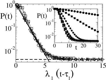
Figure 1: Main plot: Purity of the reduced density matrix for $N_{1}=N_{2}=512$, $K_{1}=K_{2}\in[4,12]$, and $\epsilon=4$ giving $2\Gamma=13.6\gg\lambda_{1}=\lambda_{2}$. Data have been calculated from 20 different initial states. The time axis has been shifted by the onset time $\tau_{1}$ (see text) and rescaled with $\lambda_{1}\in[0.5,1.35]$. The full line indicates $\propto\exp[-\lambda_{1}t]$, and the dashed line gives the asymptotic saturation ${\cal P}(\infty)=2N_{1}^{-1}$. Inset: Purity for $K_{1}=K_{2}=5.09$ for $\epsilon=0.2$ (circles), $0.4$ (squares), $0.8$ (diamonds), $1.6,2,3$ and $4$ (triangles).

To numerically check our results, we consider Hamiltonian (2) for two coupled kicked rotators Izr90

$$H_{i} = p_{i}^{2}/2+K_{i}\cos(x_{i})\;\sum_{n}\delta(t-nT),$$ (6a)

$${\cal U} = \epsilon\;\sin(x_{1}-x_{2}-0.33)\;\sum_{n}\delta(t-nT).$$ (6b)

The interaction potential ${\cal U}$ is long-ranged with a strength $\epsilon$ and acts at the same time as the kicks. Upon increasing $K_{i}$ the classical dynamics of the $i^{\rm th}$ particle varies from fully integrable ($K_{i}=0$) to fully chaotic [$K_{i}\gtrsim 7$, with Lyapunov exponent $\lambda_{i}\approx\ln(K_{i}/2)$]. For $1<K_{i}<7$ the dynamics is mixed. We will vary $K_{1,2}\in[3,12]$ to get a maximal variation of $\lambda_{i}$, while making sure that both $\psi_{1}$ and $\psi_{2}$ lie in the chaotic sea. We follow the usual quantization procedure on the torus $x,p\in(-\pi,\pi)$. The bandwidth and level spacing are given by $B_{2}=4\pi$, $\delta_{2}=4\pi/N^{2}$, and we numerically extracted $\Gamma\simeq 0.43\epsilon^{2}$ from exact diagonalization calculations of the local spectral density of states. The time evolved density matrix is computed by means of fast fourier transforms Izr90 . The algorithm requires only ${\cal O}(N\ln N)$ operations, which allowed us to reach system sizes up to $N_{1,2}=2048$, more than one order of magnitude larger than any previously investigated case.

The behavior of ${\cal P}(t)$ is shown in Fig. 1. First, it is seen that as $\epsilon$ increases, the rate of entanglement generation also increases, up to some value $\epsilon_{c}$, after which it saturates. We have found that (i) prior to saturation, ${\cal P}(t)$ decays exponentially with a rate $\approx 0.85\epsilon^{2}$, provided $\Gamma=0.43\epsilon^{2}>\delta_{2}=4\pi/N^{2}$ is satisfied, and that (ii) $\epsilon_{c}$ behaves consistently with Eq. (5). Second, Fig. 1 shows how ${\cal P}(t)$ behaves for fixed $\epsilon>\epsilon_{c}$ upon variation of the Lyapunov exponents $\lambda_{1}=\lambda_{2}$. The rescaling of the time axis $t\rightarrow\lambda_{1}t$ allows to bring together six curves with $\lambda_{1}\in[0.5,1.35]$, varying by almost a factor three. Third, Fig. 1 shows that in the chaotic regime considered here with $N_{1}=N_{2}$, ${\cal P}(t\rightarrow\infty)=2N_{1}^{-1}$. These numerical data fully confirm our main results, Eqs. (4) and (5).

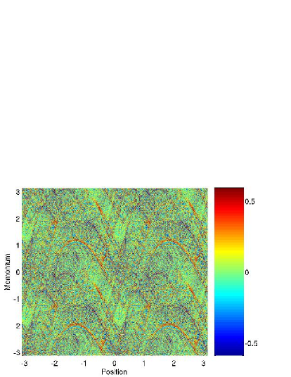
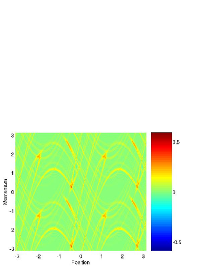
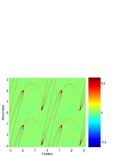
Figure 2: (Color online) Phase-space plots for a classical distribution (top left), uncoupled (top right) and coupled (bottom left and right, $\epsilon=4$) quantum Wigner distributions, after five iterations of the kicked rotator map of Eqs. (2) and (6). In all cases, the system has $K_{1}=3.09$, and the initial distributions are Gaussian centered in the chaotic sea at $(x,p)=(1,2)$. Bottom panels: Wigner functions for the quantum system coupled to a second kicked rotator with $K_{2}=100$. One has $2\Gamma=13.6>\lambda_{2}\gg\lambda_{1}$, so that the purity behaves as ${\cal P}(t)\simeq\exp[-\lambda_{1}t]$. The left panel has $N_{1}=N_{2}=512$ and the right panel has $N_{1}=N_{2}=2048$. The presence of ghost images in the Wigner function is an artifact of the boundary conditions Dittrich .

We next turn our attention to the quantum-classical correspondence in phase space. We compare in Fig. 2 the Liouville evolution of a classical distribution with that of the Wigner function $W_{1}({\bf p},{\bf q};t)=(2\pi\hbar)^{-d}\int{\rm d}{\bf x}\exp[i{\bf p}{\bf x}]\rho_{1}({\bf q}+{\bf x}/2,{\bf q}-{\bf x}/2;t)$. The latter is quantum-mechanically evolved from a localized wavepacket with the same initial location and extension as the classical distribution. Three quantum phase-space plots are shown: (i) (top right) for a free system, $\epsilon=0$; (ii) and (iii) (bottom left and right) for a coupled system $\epsilon=4$, in the regime ${\cal P}(t)\simeq\exp[-\lambda_{1}t]$. The bottom left panel has a system size $N_{1}=N_{2}=512$ while the bottom right panel has $N_{1}=N_{2}=2048$. All plots show phase-space distributions after 5 kicks, a duration comparable to $\tau_{\rm E}$. Two things are clear from these figures. First, a coupling is necessary and sufficient to achieve phase-space quantum-classical correspondence. Second, the correspondence becomes better as we move deeper in the semiclassical regime, even though the interaction Hamiltonian vanishes in that limit !

One key issue is whether the observed classical entanglement rate translates into a Lyapunov decoherence rate for systems coupled to a true environment. The latter differs from a coupling to a single particle in that it has much shorter time scales, it has a much bigger Hilbert space, and it cannot be initially prepared in a pure Gaussian wavepacket. We can take these conditions into account in our semiclassical approach by considering (i) $\lambda_{2}\gg\lambda_{1}$, (ii) $N_{2}\rightarrow\infty$ and (iii) taking an initial mixed environment density matrix $\rho_{\rm env}=\sum_{a}|\phi_{a}|^{2}|a\rangle\langle a|$, with $\langle{\bf x}|a\rangle$ being nonoverlapping Gaussian wavepackets. The result is that Eq. (4) is replaced by

$${\cal P}(t) \simeq \alpha_{1}\Theta(t>\tau_{1})\exp[-\lambda_{1}t]+\exp[-2\Gamma t]$$ (7)

$$+\Theta(t>\tau^{(1)}_{\rm E})N_{1}^{-1}.$$

The dynamical Lyapunov decay of the purity seems to survive in the case of a particle coupled to an environment. We have obtained numerical confirmation of Eq. (7) which we do not present here.

We stress in conclusion that one advantage of our approach is that ${\cal P}(t)$ is directly calculated, without the step of numerically integrating a differential equation for $\rho_{1}(t)$. Future works should focus on multipartite entanglement and decoherence by an environment consisting of many coupled dynamical systems.

This work has been supported by the Swiss National Science Foundation.

References

- (1) E. Joos, H.D. Zeh, C. Kiefer, D. Giulini, J. Kupsch, I.-O. Stamatescu, Decoherence and the Appearance of a Classical World in Quantum Theory, 2nd Ed. (Springer, Berlin 2003).
- (2) W.H. Zurek, Rev. Mod. Phys. 75, 715 (2003).
- (3) S. Habib, K. Shizume, and W.H. Zurek, Phys. Rev. Lett. 80, 4361 (1998).
- (4) F. Toscano, R.L. de Matos Filho, and L. Davidovich, Phys. Rev. A 71, 010101(R) (2005).
- (5) A.K. Pattanayak, Phys. Rev. Lett. 83, 4526 (1999); D. Monteoliva and J.P. Paz, Phys. Rev. Lett. 85, 3373 (2000).
- (6) Refs. entropy show entropy production rates without varying the Lyapunov exponent.
- (7) R.A. Jalabert and H.M. Pastawski, Phys. Rev. Lett. 86, 2490 (2001).
- (8) Ph. Jacquod, P.G. Silvestrov, and C.W.J. Beenakker, Phys. Rev. E 64, 055203(R) (2001).
- (9) F.M. Cucchietti, D.A.R. Dalvit, J.P. Paz, and W.H. Zurek, Phys. Rev. Lett. 91, 210403 (2003).
- (10) Ph. Jacquod, Phys. Rev.Lett. 92, 150403 (2004).
- (11) K. Furuya, M.C. Nemes, and G.Q. Pellegrino, Phys. Rev. Lett. 80, 5524 (1998); J.N. Bandyopadhyay and A. Lakshminarayan, Phys. Rev. Lett 89, 060402 (2002); M. Žnidarič and T. Prosen, J. Phys. A 36, 2463 (2003); R.M. Angelo and K. Furuya, Phys. Rev. A 71, 042321 (2005); M. Lombardi and A. Matzkin, quant-ph/0506188.
- (12) P.A. Miller and S. Sarkar, Phys. Rev. E 60, 1542 (1999).
- (13) A. Tanaka, H. Fujisaki, and T. Miyadera, Phys. Rev. E 66, 045201(R) (2002).
- (14) M. Žnidarič and T. Prosen, Phys. Rev. A 71, 032103 (2005).
- (15) A.R. Kolovsky, Phys. Rev. Lett. 76, 340 (1996).
- (16) There are subtleties related to averaging, so that are somewhat smaller than, but proportional to the Lyapunov exponents, see P.G. Silvestrov, J. Tworzydlo, and C.W.J. Beenakker, Phys. Rev. E 67, 025204(R) (2003).
- (17) F.M. Izrailev, Phys. Rep. 196, 299 (1990).
- (18) A. Arguelles and T. Dittrich, Physica A 356, 72 (2005).