Entanglement quantifiers and phase transitions

Abstract

By the topological argument that the identity matrix is surrounded by a set of separable states follows the result that if a system is entangled at thermal equilibrium for some temperature, then it presents a phase transition (PT) where entanglement can be viewed as the order parameter. However, analyzing several entanglement measures in the 2-qubit context, we see that distinct entanglement quantifiers can indicate different orders for the same PT. Examples are given for different Hamiltonians. Moving to the multipartite context we show necessary and sufficient conditions for a family of entanglement monotones to attest quantum phase transitions.

I Introduction

The study of phase transitions under the view of exclusively quantum correlations has hooked the interest of the quantum information community recently ON ; ABV . Linking entanglement and (quantum) phase transitions (PTs) is tempting since PTs are related to correlations of long range among the system’s constituents Yang . Thus expecting that entanglement presents a peculiar behavior near criticality is natural.

Recent results have shown a narrow connection between entanglement and critical phenomena. For instance, bipartite entanglement has been widely investigated near to singular points for exhibit interesting patterns ON ; ABV . The localizable entanglement LocEnt has been used to show certain critical points that are not detected by classical correlation functions VDC04 . The negativity and the concurrence quantifiers were shown to be quantum-phase-transitions witnesses LA . Furthermore, closely relations exist between entanglement and the order parameters associated to the transitions between a normal conductor and a superconductor and between a Mott-insulator and a superfluid Brab .

The main route that has been taken in order to capture these ideas is through the study of entanglement in specific systems. However it is believed that a more general picture can be found. Here, we go further in this direction starting from the generic result that, for a bipartite system at thermal equilibrium with a reservoir, there exist two distinct phases, one in which some entanglement is present and another one where quantum correlations completely vanish. We then exemplify this result with 2-qubit systems subjected to different Hamiltonians and curiously it is viewed that, by choosing different entanglement quantifiers , one attributes different orders to the phase transition.

Although multipartite entanglement also plays an important role in many-body phenomena (its is behind some interesting effects such as the Meissner effect Meis , the high-temperature superconductivity high-Tc , and superadiance Dicke ), rare results linking it to PTs exist. Crossing this barrier is also a goal of this Letter. For that, we give necessary and sufficient conditions to a large class of multipartite entanglement quantifiers to signal singularities in the ground state energy of the system. We finish this work discussing a recently introduced quantum phase transition, the geometric phase transition, which takes place when a singularity in the boundary of the set of entangled states exists.

A phase transition occurs when some state function of a system presents two distinct phases, one with a non-null value and another one in which this function takes the null value LL . Such a function is called an order parameter for the system. However one can think that this is a very tight definition and want to define a PT as a singularity in some state function of the system due to changes in some parameter (coupling factors in the Hamiltonian, temperature, etc). By extension, this function is also called the order parameter of the PT. Note that the first definition of PT is a special case of the latest one. When the singularity expresses itself as a discontinuity in the order parameter we say that we are dealing with a discontinuous PT. If the discontinuity happens in some of the derivatives of the order parameter, say the $n^{th}$-derivative, it is said to be a $n^{th}$-order PT, or a continuous PT. In this paper we will consider entanglement as a state function and see that it can present a singularity when some parameter of the problem changes. Thus, we make a more general discussion about when a given entanglement quantifier, or some of its derivatives, can present a discontinuity.

II The entangled$\rightarrow$disentangled transition

The first phase transition we will discuss is when a system is in thermal equilibrium with a reservoir. This system can show two phases: one separable and other entangled. The following question raises: is this transition smooth? We will show that the answer for this question depends on the entanglement quantifier adopted.

Let us first revisit a very general result following just from a topological argument. Given a quantum system with Hamiltonian $H$, its thermal equilibrium state is given by $\rho(T)=\frac{\exp(-\beta H)}{Z}$, where $Z=\mathrm{Tr}\exp(-\beta H)$ is the partition function and $\beta=(k_{B}T)^{-1}$, $k_{B}$ denoting the Boltzmann constant and $T$ the absolute temperature. This state is a continuous function of its parameters. If the space state of the system has finite dimension $d$, then $\lim_{T\rightarrow\infty}\rho(T)=\frac{I}{d}$, where $I$ denotes the identity operator. For multipartite systems, $\frac{I}{d}$ is an interior point in the set of separable states ZHSL , i.e., it is separable and any small perturbation of it is still separable. The thermal equilibrium states $\rho(T)$ can be viewed as a continuous path on the density matrix operators set, ending at $\frac{I}{d}$. So if for some temperature $T_{e}$ the state $\rho(T_{e})$ is non-separable, there is a finite critical temperature $T_{c}>T_{e}$ such that $\rho(T_{c})$ is in the boundary of the set of separable states. An important class of examples is given by the systems with entangled ground state, i.e., $T_{e}=0$.

It is clear that the entanglement $E$ of the system will present a singularity at $T_{c}$. Thus $E$ can be viewed as a true order parameter in the commented PT. Moreover let us explore a little bit more the result that “thermal-equilibrium entanglement vanishes at finite temperature”FMB ; Rag . It will be shown that different entanglement quantifiers attribute different orders for this PT. For that we will show an entanglement quantifier that is discontinuous at $T_{c}$, two others presenting a discontinuity at its first derivative (asserting a $1^{th}$-order PT), and another one in which the discontinuity manifests itself in $\frac{d^{2}E(\rho)}{dT^{2}}|_{T=T_{c}}$ (asserting a $2^{nd}$-order PT).

As the first example take the Indicator Measure, $IM(\rho)$, defined as 1 for entangled states and 0 for separable ones. Although $IM$ is an entanglement monotone it is quite weird once it is a discontinuous function itself. Of course $IM$ presents a discontinuity at $T=T_{c}$, i.e., when $\rho$ crosses the border between the entangled and the disentangled-states world.

However it is interesting to study some best behavioured and well-accepted entanglement monotones, and we will do that through some examples in the 2-qubit context. Take the concurrence $C$, the entanglement of formation $E_{f}$ and the negativity $N$. These three functions are able to quantify entanglement properly although, as it will be seen, in different manners. The entanglement of formation was proposed by Bennett et al.Ef as the infimum of mean pure state entanglement among all possible ensemble descriptions of a mixed state $\rho$. The concurrence was developed by Wootters and collaborators Woo in the context of trying to figure out a feasible way to calculate the entanglement of formation. Thus $E_{f}$ and $C$ are connected by

$$E_{f}(\rho)=H_{2}\left(\frac{1}{2}+\frac{1}{2}\sqrt{1-C^{2}(\rho)}\right),$$ (1)

where $H_{2}(x)=-x\log x-(1-x)\log(1-x)$ and it is assumed that $0\log 0=0$. The concurrence can be defined by

$$C(\rho)=\max(0,\lambda_{1}-\lambda_{2}-\lambda_{3}-\lambda_{4}),$$ (2)

with $\lambda_{i}$ being the square roots of the eigenvalues of the matrix $\rho(\sigma_{y}\otimes\sigma_{y})\rho^{*}(\sigma_{y}\otimes\sigma_{y})$ in decreasing order and $\sigma_{y}$ is the Pauli matrix.

On the other hand the negativity uses the idea of partial transpose to calculate entanglement VW ; ZHSL . It can be defined as

$$N(\rho)=\|\rho^{T_{A}}\|-1,$$ (3)

where the subscript $T_{A}$ indicates the partial transpose operation and $\|\star\|$ means the trace norm. Alternatively, one can define the logarithmic negativity as VW ; ZHSL $E_{\mathcal{N}}(\rho)=\log_{2}(1+N(\rho))$.

Let us use these quantifiers to study the entanglement of thermal-equilibrium states,

$$\rho=\frac{\exp(-\beta H)}{Z},$$ (4)

subject to a completely non-local Hamiltonian of the form Dur+

$$H=x\sigma_{x}\otimes\sigma_{x}+y\sigma_{y}\otimes\sigma_{y}+z\sigma_{z}\otimes\sigma_{z}.$$ (5)

Note that the 1D 2-qubit Heisenberg chain is a particular case of (5) when $x=y=z=J$ ($J<0$ being the ferromagnetic and $J>0$ the antiferromagnetic cases). The results are plotted in Figs. 1, 2, and 3.

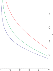
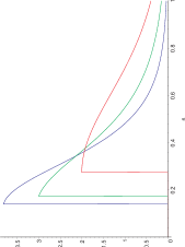
Figure 1: (Color online) Above: $C(\rho)$ vs. $\beta$ for $x=1,y=1,z=1$ (red); $x=3,y=1,z=1$ (green); and $x=3,y=2,z=1$ (blue). Below:$\frac{dC(\rho)}{d\beta}$ vs. $\beta$ for the same values of $x,y,$ and $z$. $C$ shows a PT of $1^{st}$ order (its 1st derivative is discontinuous). In the cases considered $C(\rho)$=$N(\rho)$, and the conclusions are also valid for the negativityVer .

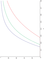
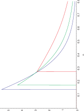
Figure 2: (Color online) Above: $E_{\mathcal{N}}(\rho)$ vs. $\beta$ for $x=1,y=1,z=1$ (red); $x=3,y=1,z=1$ (green); and $x=3,y=2,z=1$ (blue). Below: $\frac{dE_{\mathcal{N}}(\rho)}{d\beta}$ vs. $\beta$ for the same values of $x,y,$ and $z$.

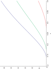
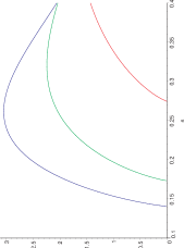
Figure 3: (Color online) Above: $E_{f}(\rho)$ vs. $\beta$ for $x=1,y=1,z=1$ (red); $x=3,y=1,z=1$ (green); and $x=3,y=2,z=1$ (blue). Below:$\frac{dE_{f}(\rho)}{d\beta}$ vs. $\beta$ for the same values of $x,y,$ and $z$.

An interesting conclusion following from the figures is that according to $E_{F}$ the transition is of $2^{nd}$ order, according to $C$ (and $N$ as well) and $E_{\mathcal{N}}$ it is of $1^{st}$ order, and remember that, according to $IM$ all transitions are discontinuous. In fact it is possible to see, directly from its definition, that $E_{\mathcal{N}}$ will always present a discontinuity in the same derivative as $N$. For this aim we can write:

$$\frac{dE_{\mathcal{N}}(\beta)}{d\beta}=\frac{1}{(1+N(\beta))\ln 2}\frac{dN(\beta)}{d\beta}.$$ (6)

Similarly, the relation between $E_{f}$ and $C$ can be also verified analytically. The derivative of $E_{f}$ with respect to $\beta$ is

$$\frac{dE_{f}(\beta)}{d\beta}=\frac{C(\beta)}{2\sqrt{1-C^{2}(\beta)}}\log\left(\frac{1-\sqrt{1-C^{2}(\beta)}}{1+\sqrt{1-C^{2}(\beta)}}\right)\frac{dC(\beta)}{d\beta}.$$ (7)

So it is possible to see that, even $C(\beta)$ being singular at $\rho_{c}$ (it is, when $T=T_{c}$), the singularity manifests itself on $E_{f}(\beta)$ only to the next order.

In fact, this situation resembles that in percolation theory, when different “percolation quantifiers” like probability of percolation, the mean size of the clusters, and the conductivity between two points show different critical behaviourSA .

III Multipartite entanglement as indicator of quantum phase transitions

In Ref.LA , the authors show that the concurrence and the negativity serve themselves as quantum-phase-transition indicators. This is because, unless artificial occurrences of non-analyticities, these quantifiers will present singularities if a quantum phase transition happens. An extend result for another bipartite entanglement quantifiers is presented in ref.LA2 . In the same context, Rajagopal and Rendell offer generalizations of this theme to the more general case of mixed stateRR05 .

By following the same line of research we now extend the previous results to the multipartite case. We will see that it is possible to establish some general results, similar to Ref.LA , also in the multipartite scenario. We can use for this aim the Witnessed Entanglement, $E_{W}(\rho)$, to quantify entanglement FB (this way of quantifying entanglement includes several entanglement monotones as special cases, such as the robustness and the best separable approximation measure). Before giving the definition of $E_{W}$ we must review the concept of entanglement witnesses. For all entangled state $\rho$ there is an operator that witnesses its entanglement through the expression $\mathrm{Tr}(W\rho)<0$ with $\mathrm{Tr}(W\sigma)\geq 0$ for all $k$-separable states $\sigma$ (we call $k$-separable every state that does not contain entanglement among any $m>k$ parts of it, and denote this set $S_{k}$) FB . We are now able to define $E_{W}$. The witnessed entanglement of a state $\rho$ is given by

$$E_{W}^{k}(\rho)=\max\{0,-\min_{W\in\mathcal{M}}Tr(W\rho)\},$$ (8)

where the choice of $\mathcal{M}$ allows the quantification of the desired type of entanglement that $\rho$ can exhibit. The minimization of $\mathrm{Tr}(W\rho)$ represents the search for the optimal entanglement witness $W_{opt}$ subject to the constraint $W\in\mathcal{M}$. The interesting point is that by choosing different $\mathcal{M}$, $E_{W}$ can reveal different aspects of the entanglement geometry and thus quantify entanglement under several points of view. As a matter of fact, if in the minimization procedure in (8) it is chosen to search among witnesses $W$ such that $\mathrm{Tr}(W)\leq I$ ($I$ is the identity matrix), $E_{W}$ is nothing more than the generalized robustness, an entanglement quantifier VT with a rich geometrical interpretation Nos2 ; Nos3 . Other choices of $\mathcal{M}$ would reach other known entanglement quantifiers FB . Moreover it is easy to see that, regardless these choices, $E_{W}$ is a bilinear function of the matrix elements of $\rho$ and of $W_{opt}$. So singularities in $\rho$ or in $W_{opt}$ cause singularities in $E_{W}(\rho)$.

At this moment we can follow Wu et al., in Ref. LA and state that, if some singularity occurring in $E_{W}$ is not caused by some artificial occurrences of non-analyticity (e.g., maximizations or some other mathematical manipulations in the expression for $E_{W}$ - see conditions a-c in Theorem 1 of Ref. LA ), then a singularity in $E_{W}$ is both necessary and sufficient to signal a PT. It is important to note that the concept of PT considered by the authors is not thermal equilibrium PT: the PT’s discussed by them are that linked with non-analyticities in the derivatives of the ground state energy with respect to some parameters as a coupling constant. On the other hand it is also important to highlight that our result implies a multipartite version of theirs. Moreover, the use of $E_{W}$ to studying quantum phase transitions can result in a possible connection between critical phenomena and quantum information, as $E_{W}$ (via the robustness of entanglement) is linked to the usefulness of a state to teleportation processes Brac .

We can go further in the concept of a PT and study the cases where $E_{W}$ presents a singularity. An interesting case is when a discontinuity happens in $W_{opt}$ and not in $\rho$. This can happen for example if the set $S_{k}$ presents a sharp shape, situation in which occurs the recently introduced geometric phase transitionNos2 , where the PT is due the geometry of $S_{k}$. Besides the interesting fact that a new kind of quantum phase transition can occur, the geometric PT could be used to study the entanglement geometry. This can be made by smoothly changing some density matrix and establishing whether $E_{W}$ reveals some singularity. Furthermore, $E_{W}$ can be experimentally evaluated, as witness operators are linked with measurement processes GHB ; TG and has been used to attest entanglement experimentally BEK . So, the geometry behind entanglement can even be tested experimentally. A more detailed study of this issue is given in Ref.Nos2 .

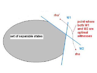
Figure 4: (Color online)The red (dot) line represents the way followed by $\rho$ when some parameter of the systems is changed. Geometrically, entanglement witness can be interpreted as tangent hyperplanes to $S_{k}$. At a certain point both witnesses $W1$ and $W2$ are optimal for $\rho$. At this point there is a singularity in $E_{W}(\rho)=-Tr(W_{1or2}\rho)$.

IV Conclusion

Summarizing, we have shown that entangled thermal-equilibrium systems naturally present a phase transition when heated: the entanglement-disentanglement transition. However different entanglement quantifiers lead with this PT differently, in the sense that, according to some of them the PT is of $1^{st}$-order (e.g., the negativity and concurrence), $2^{nd}$-order (e.g., the entanglement of formation), and even though discontinuous (e.g., the indicator measure). With these ideas in mind it is tempting to make some questions: Is the PT showed here linked with some other physical effect other than just vanishing quantum correlations? In other words, which macroscopically observed PT have entanglement as order parameter? Can the way in which entanglement quantifiers lead with PT be considered a criterion for choosing among them? Is there “the good” quantifier to deal with such PT? We hope our present contribution can help in answering these questions.

Recent discussions have shown that the entanglement-disentanglement transition is behind important quantum phase transitions Brab . So similar analysis can also be performed in different contexts other than temperature increasing. Decoherence processes could be a rich example.

- (1) T. J. Osborne and M. A. Nielsen, Phys. Rev. A66, 032110 (2002); A. Osterloh, L. Amico, G. Falci, and R. Fazio, Nature 416, 608 (2002); J. I. Latorre, E. Rico, and G. Vidal, Quant. Inf. and Comp. 4, 048 (2004); G. Vidal, J. I. Latorre, E. Rico, and A. Kitaev, Phys. Rev. Lett. 90, 227902 (2003); T. Roscilde, P. Verrucchi, A. Fubini, S. Haas, and V. Tognetti, Phys. Rev. Lett. 93, 167203 (2004); T. Roscilde, P. Verrucchi, A. Fubini, S. Haas, and V. Tognetti, Phys. Rev. Lett. 94, 147208 (2005); D. Larsson and H. Johannesson, Phys. Rev. Lett. 95, 196406 (2005).
- (2) M. C. Arnesen, S. Bose, and V. Vedral, Phys. Rev. Lett. 87, 017901 (2001).
- (3) C. N. Yang, Rev. Mod. Phys. 34, 694 (1962).
- (4) F. Verstraete, M. Popp , and J. I. Cirac, Phys. Rev. Lett. 92, 027901 (2004); M. Popp, F. Verstraete, M. A. Martín-Delgado, and J. I. Cirac, Phys. Rev. A71, 042306 (2005).
- (5) F. Verstraete, M. A. Martín-Delgado, and J. I. Cirac, Phys. Rev. Lett. 92, 087201 (2004).
- (6) L.-A. Wu, M. S. Sarandy, and D. A. Lidar, Phys. Rev. Lett. 93, 250404 (2004).
- (7) F. G. S. L. Brandão, New J. Phys. 7, 254 (2005). .
- (8) V. Vedral, e-print quant-ph/0410021.
- (9) V. Vedral, New J. Phys. 6, 102 (2004).
- (10) N. Lambert, C. Emary, and T. Brandes, Phys. Rev. Lett. 92, 073602 (2004).
- (11) L. D. Landau and E. M. Lifshitz, Statistical Physics (Addison-Wesley, Reading, Mass., 1969).
- (12) K. Życzkowski, P. Horodecki, A. Sanpera, and M. Lewenstein, Phys. Rev. A 58, 883 (1998).
- (13) B. V. Fine, F. Mintert, and A. Buchleitner, Phys. Rev. B 71, 153105 (2005).
- (14) G. A. Raggio, J. Phys. A: Math. Gen. 39, 617 (2006); O. Osenda and G. A. Raggio, Phys. Rev. A72, 064102 (2005).
- (15) G. Vidal,J. Mod. Opt. 47, 355 (2000).
- (16) C. H. Bennett, H. J. Bernstein, S. Popescu, and B. Schumacher Phys. Rev. A 53, 2046 (1996).
- (17) W. K. Wootters, Phys. Rev. Lett. 80, 2245 (1998). S. Hill and W. K. Wootters, Phys. Rev. Lett. 78, 5022 (1997).
- (18) J. Eisert, PhD thesis University of Potsdam, January 2001; G. Vidal and R.F. Werner, Phys. Rev. A 65, 032314 (2002); K. Audenaert, M. B. Plenio and J. Eisert, Phys. Rev. Lett. 90, 027901 (2003); M. B. Plenio, Phys. Rev. Lett. 95, 090503 (2005).
- (19) W. Dür, G. Vidal, J.I. Cirac, N. Linden, and S. Popescu, Phys. Rev. Lett. 87, 137901 (2001). C. H. Bennett et al., Phys. Rev. A 66, 012305 (2002).
- (20) F. Verstraete et. al., J. Phys. A: Math. Gen. 34, 10327 (2001).
- (21) D. Stauffer and A. Aharony, Introduction to Percolation Theory (Taylor and Francis, 1992).
- (22) L.-A. Wu, M. S. Sarandy, D. A. Lidar, and L. J. Sham, eprint quant-ph/0512031.
- (23) A. K. Rajagopal and R. W. Rendell, eprint quan-ph/0512102.
- (24) F. G. S. L. Brandão, Phys. Rev. A 72, 022310 (2005).
- (25) M. Steiner. Phys. Rev. A 67, 054305 (2003). G. Vidal and R. Tarrach. Phys. Rev. A 59, 141 (1999).
- (26) D. Cavalcanti, F.G.S.L. Brandão, and M.O. Terra Cunha, e-print quant-ph/0510068.
- (27) D. Cavalcanti, F.G.S.L. Brandão, and M.O. Terra Cunha, Phys. Rev. A72, 040303(R) (2005).
- (28) F. G. S. L. Brandão, e-print quant-ph/0510078. Ll. Masanes, e-print quant-ph/0508071.
- (29) O. Gühne et al., Phys. Rev. A 66, 062305 (2002).
- (30) G. Tóth and O. Gühne, Phys. Rev. Lett. 94, 060501 (2005).
- (31) M. Bourennane et al., Phys. Rev. Lett. 92, 087902 (2004); M. Barbieri et al., Phys. Rev. Lett. 91 227901 (2003).