Quantum extension of European option pricing based on the Ornstein-Uhlenbeck process

Abstract

In this work we propose a option pricing model based on the Ornstein-Uhlenbeck process. It is a new look at the Black-Scholes formula which is based on the quantum game theory. We show the differences between a classical look which is price changing by a Wiener process and the pricing is supported by a quantum model.

PACS numbers: 02.50.-r, 02.50.Le, 03.67.-a, 03.65.Bz

Introduction

Option trading experienced a gigantic growth with the creation of the Chicago Board of Options Exchange in 1973. Since this moment there is an on going demand for derivatives instruments. And this induce financiers, mathematicians and physicians to the wider and deeper research of the finance instruments of the price changing dynamics. Owing to the fact, that an analogy has been discovered between market prices behavior and the dust particle motion model by a Wiener process. This observation revolutionized derivatives pricing by developing a pioneering formula for evaluating paying no dividend stock options, whose creators in 1997 have way a Nobel Prize for. The Black-Scholes formula is the most popular deployed computational model. We propose an alternative description of the time evolution of market price making corrections in the Wiener-Bachelier model and which follows from the Ornstein-Uhlenback process. This process has been successfully used by Vasicek in 1997 for modeling the short time interest rate. Modifications have already been propose in works e.g. [1, 2]. In the latest year have appeared variant a game theory based on the quantum formalism [3] it qualitatively broaden the capabilities of this discipline describing the strategy which can not be realized in classical models. Game theory describes conflict scenarios between a number of individuals or groups who try to maximize their own profit, or minimize profits made by their opponents. However, by adopting quantum trading strategies it seems that players can make more sophisticated decisions, which may lead to better profit opportunities. The success of the quantum information theory (quantum algorithm or quantum cryptography) could make these futuristic-sounding quantum trading systems a reality, due to quantum computer development it will be possible to better model the market. Quantum market model exist and in this kind of market we can valuation the derivative instrument. The pricing of derivative securities as a problem of quantum mechanics presented already Belal E. Baaquie, see [5].

In the first section we are going to quote the logarithmic equation which fulfills the logarithmic stock price and we will be able to find the formula of these prices. In the second section we will be able to find the European option price supported by Wiener-Bachelier model and we will be able to receive the famous formula of Black-Scholes. Next we give the analogical probability like in the first section, but it will be supported by Ornstein-Uhlenbeck process. In the fourth section we interpret of the Ornstein-Uhlenbeck model in terms of quantum market games theory as a non-unitary thermal tactic [4]. In the fifth section with a little help of quantum model we find a model which describes the European option pricing.

1 Price changing model as a Wiener process

In 1900 Louis Bachelier in his dissertation showed that the market prices behaves like a dust particles performing a one-dimensional Brownian motion. Nowadays, we are used to approximate the logarithmic price movements a Wiener process. These movements can be described by system of equations [6]

$$\left\{\begin{array}[]{ll}\hbox{$dX_{t}=\sigma X_{t}\,dB_{t}+\mu X_{t}dt$}\\ \hbox{$X_{0}=x_{0}$}\\ \end{array}\right.,$$

where $t$ equal time, $\mu$ is the growing rate (drift), $\sigma$ is a volatility rate and $B_{t}$ represent the standard Brownian motion. In the above process for the exact moment $t>0$, the probability density function of finding the randomly moving particle at the point $x$ (price logarithm) is given as the Gaussian function

$$f(x,t):=\frac{1}{\sqrt{2\pi t}\,\sigma}\,\,\text{e}^{-\frac{(x-\mu t)^{2}}{2\sigma^{2}t}}.$$ (1)

Because the time evolution of the logarithm of stock price is described by a Winer process, its current price $S_{t}$ is given by

$$S_{t}=S_{0}\text{e}^{\mu t+\sigma B_{t}},$$

where $S_{0}$ is the stock price in the $t=0$ moment. Assuming that we are dealing with effective market and is no possibility of arbitrage, and assuming that the parameters are fixed in this model, the necessary estimators of these parameters we can be found by econometric methods. The mean value of the stock price at the moment $t$ must equal $S_{0}$ and the riskless interest rate $r$ is constant in the period $\left[0,t\right]$. So, if accepting the continuous capitalization, we get

$$S_{0}\text{e}^{rt}=\mathit{E}S_{t}=S_{0}\text{e}^{\mu t}\mathit{E}\text{e}^{\sigma B_{t}}=S_{0}\text{e}^{\mu t+\frac{1}{2}\sigma^{2}t}.$$

Hence

$$\mu=r-\tfrac{\sigma^{2}}{2}\,.$$ (2)

Substituting (2) to (1) we are get distribution of the logarithm of stock price

$$f(x,t)=\frac{1}{\sqrt{2\pi t}\,\sigma}\,\text{e}^{-\frac{(x-(r-\frac{1}{2}\sigma^{2})t)^{2}}{2\sigma^{2}t}}.$$ (3)

The above distribution is called the distribution of the Wiener-Bachelier. The function (3) fulfills a diffusion equation with an arbitrage forbidding drift.

2 The Wiener-Bachelier option pricing model

Let us consider the European call option on company’s stock which is not paying a dividend, with the strike price of $K$ and the maturity time $T$. Let us calculate the current value of this option. The price of this option at the moment $T$ is equal $[S_{T}-K]^{+}:=\max\{S_{T}-K,0\}$, because of $K\negthinspace>\negthinspace S_{T}$ so this call option want be exercise and hence to that its value will be $0$ [7]. The option fair price at $T\negthinspace=\negthinspace 0$ should be equal to the discounted mean value (assume that the interest rate $r$ is constant $[0,T]$ in the term)

$$c=\text{e}^{-rT}\mathit{E}[S_{T}-K]^{+}=\text{e}^{-rT}\int_{-\infty}^{\infty}[S_{0}\text{e}^{x}-K]^{+}f(x,T)\,dx$$ (4)

$$=\text{e}^{-rT}\int_{-\ln\frac{S_{0}}{K}}^{\infty}(S_{0}\text{e}^{x}-K)\,\frac{1}{\sqrt{2\pi T}\,\sigma}\,\text{e}^{-\tfrac{(x-(r-\frac{1}{2}\sigma^{2})T)^{2}}{2\sigma^{2}T}}dx\,.$$

Calculated of integral over the $dx$, we are getting the formula

$$c=S_{0}N(\tfrac{\ln\frac{S_{0}}{K}+(r+\frac{\sigma^{2}}{2})\,T}{\sigma\sqrt{T}})-Ke^{-rT}N(\tfrac{\ln\frac{S_{0}}{K}+(r-\frac{\sigma^{2}}{2})\,T}{\sigma\sqrt{T}})\,.$$

In this way, we have received the famous Black-Scholes formula on the value European call option, where the cumulative distribution function $N$ is the standard normal distribution.

3 The model of Ornstein-Uhlenbeck

The Ornstein-Uhlenbeck process describe a particle behavior called by physicists the Rayleigh particle [8]. It can be described by the system of equations

$$\left\{\begin{array}[]{ll}\hbox{$dX_{t}=\sigma\sqrt{2q}\,dB_{t}-qX_{t}dt$}\\ \hbox{$X_{0}=x_{0}$}\\ \end{array}\right.,$$

where $q$ and $\sigma$ are some positive constant, whereas $B_{t}$ means the Brownian motion. The transition probability density of the random variable $X$ in the time $t$, which is a fundamental solution of the corresponding the Fokker-Planck equation [9], is given by the formula

$$f_{q}(x,t):=\frac{1}{\sqrt{2\pi(1-\text{e}^{-2qt})}\,\sigma}\,\,\text{e}^{-\frac{(x-x_{0}\text{e}^{-qt})^{2}}{2\sigma^{2}(1-\text{e}^{-2qt})}}\,.$$ (5)

The parameter $q$ modifies the time scale in which we can examine the particle place. For very small values of $q$ we obtain the short time scale $\gamma\negthinspace:=\negthinspace qt$ [8] in which the Ornstein-Uhlenbeck process, which describe the velocity evolution of the Rayleigh particle, approximate to the Brownian motion.
If we assume that the logarithmic price of the stock behaves similarly to the Rayleigh particle and we also take effective market into consideration, so we can count the logarithmic distribution of an stock based on Ornstein-Uhlenbeck model. Let us $x=\ln S_{t}$ for $t\negthinspace>\negthinspace 0$. Then, making calculations similar for the Brown particle, we get

$$S_{0}\text{e}^{rqt}=\mathit{E}S_{t}=\int_{-\infty}^{\infty}S_{0}\text{e}^{x}f_{q}(x,t)\,dx=S_{0}\text{e}^{(x_{0}+\sigma^{2}\sinh qt)\,\text{e}^{-qt}},$$

and

$$x_{0}(t)=rqt\,\text{e}^{qt}-\sigma^{2}\sinh qt\,.$$

In result the probability density of the logarithm of stock price is

$$f_{q}(x,t)=\frac{1}{\sqrt{2\pi(1-\text{e}^{-2qt})}\,\sigma}\,\,\text{e}^{-\frac{(x-rqt+\sigma^{2}\text{e}^{-qt}\sinh qt)^{2}}{2\sigma^{2}(1-\text{e}^{-2qt})}}\,.$$ (6)

Let us see that, $f_{q}\rightarrow f$ near $t\rightarrow 0$, see Appendix. While near $t\rightarrow\infty$ function $f_{q}(x-rqt,t)$ approach to Gauss factorization with the same parameters, which corresponds the price equality which result from the market expectations, so on the base of the fundamental analyze. From here the Ornstein-Uhlenback process would give the realistic situations of the market in the mezzo-scale, temporal, it means in the time where there is not enough to approximate by a Wiener-Bachelier process, but so small that in the result of the processes of economics and innovations, there has not been changed the market expectations, so like the asymptotic state of equality on the “new” one.

4 Quantum market games interpretation of Ornstein-Uhlenback model

In the quantum game theory Ornstein-Uhlenback process has the interpretation of non-unitary tactics [4], leading to a new strategy. We call tactics characterized by a constant inclination of an abstract market player (Rest of the World) to risk $\mathit{E}(H(\mathcal{P},\mathcal{Q}))\negthinspace=\negthinspace const$ and maximal entropy thermal tactics. $H$ is a Hamilton operator that specifies the model, whereas $\mathcal{P},\mathcal{Q}$ are Hermitian operators of supply and demand [4, 10]. These traders adopt such tactics that the resulting strategy form a ground state of the risk inclination operator $H(\mathcal{Y},\mathcal{Z})$. Therefor, thermal tactics are represented by an operator

$$\mathcal{R}_{\gamma}=e^{-\gamma(H(\mathcal{Y},\mathcal{Z})-\frac{1}{2})},$$

where $\mathcal{Y}\negthinspace=\negthinspace\frac{1}{\sqrt{2}}(\mathcal{P}\negthinspace-\negthinspace\mathcal{Q})$ and $\mathcal{Z}\negthinspace=\negthinspace\frac{1}{\sqrt{2}}(\mathcal{P}\negthinspace+\negthinspace\mathcal{Q})$. The variable $\mathcal{Y}$ describes arithmetic mean deviation of the logarithm of price from its expectation value. Quantum strategies create unique opportunities for making profits during intervals shorter than the characteristic thresholds for the Brownian particle. To describe the evolution of the market price in the quantum models we use the Rayleigh particle, it is the non-unitary thermal tactics approaching equilibrium state.

The variable $y$ describes the logarithmic transactional price. $\mathcal{R}_{\gamma}$ operator (tactics) transforms the strategy $\langle y|\psi\rangle\negthinspace\in\negthinspace\mathcal{L}^{2}$ and, in the $\gamma$ moment it has the form [11]

$$\mathcal{R}_{\gamma}(y,\psi):=\langle y|\mathcal{R}_{\gamma}\psi\rangle=\int_{-\infty}^{\infty}\negthinspace\negthinspace\mathcal{R}_{\gamma}(y,y^{\prime})\langle y^{\prime}|\psi\rangle dy^{\prime}\,,$$

where

$$\mathcal{R}_{\gamma}(y,y^{\prime})=\tfrac{1}{\sqrt{\pi\sigma(1-\text{e}^{-2\gamma})}}\,\,\text{e}^{{-\frac{y^{2}-{y^{\prime}}^{2}}{2\sigma}-\frac{(\text{e}^{-\gamma}y-y^{\prime})^{2}}{\sigma(1-\text{e}^{-2\gamma})}}}\,.$$

$\mathcal{R}_{\gamma}$ tactics is called the Ornstein-Uhlenbeck process. Adoption of the thermal tactics means that traders have in view minimization of the risk within the available information on the market. So we adopt such a normalization of the operator of the tactics so that the resulting strategy is its fixed point. Conditions for the fixed point these tactics allows to interpret it as probabilistic measure describe in the formula $(\ref{moja})$, see [4].

5 Option pricing based on quantum model

Let us move to the European call option pricing underlying on company’s stock which is not paying dividend and based on changing prices which are not the Brownian motion but the Ornstein-Uhlenbeck process modeled. To achieve the Black-Scholes formula, it is enough to count the integral $(\ref{pierwsza})$ for the modified density of the probability $f\negthinspace\to\negthinspace f_{q}$, assuring no arbitrage definite formula $(\ref{osta})$. The formula for the price of the option takes the form

$$c_{q}=\text{e}^{-rqT}\mathit{E}_{q}[S_{T}-K]^{+}=\text{e}^{-rqT}\int_{-\infty}^{\infty}[S_{0}\text{e}^{x}-K]^{+}f_{q}(x,T)\,dx$$ (7)

$$=\frac{1}{\sqrt{2\pi(1-\text{e}^{-2qT})}\,\sigma}\,\,\text{e}^{-rqT}\int_{-\infty}^{\infty}[S_{0}\text{e}^{x}-K]^{+}\,\text{e}^{-\frac{(x-rqT+\sigma^{2}\text{e}^{-qT}\sinh qT)^{2}}{2\sigma^{2}(1-\text{e}^{-2qT})}}\,dx$$

$$=S_{0}N(\tfrac{(rqT+\ln\tfrac{S_{0}}{K})\,\text{e}^{qt}\,+\,\sigma^{2}\sinh qt}{\sigma\sqrt{2\text{e}^{qt}\sinh qt}}\,)\,\,-\,\,\text{e}^{-rqT}KN(\tfrac{(rqT+\ln\tfrac{S_{0}}{K})\,\text{e}^{qt}\,-\,\sigma^{2}\sinh qt}{\sigma\sqrt{2\text{e}^{qt}\sinh qt}}\,)\,.$$

The difference between the logarithmic price the European call option described by the Ornstein-Uhlenback process and logarithmic price call option described by the Wiener-Bachelier process is present in Figure 1. The corrections to the Bachelier model should matter for mezzo-scale.

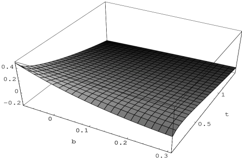
Figure 1: Function $\ln c_{q}-\ln c$, for $b=\ln\frac{S_{0}}{K}$, $r=0$, $\sigma=q=1$ .

6 Final remarks

We have proposed the alternative description of the time evolution of market price that is inspired by quantum mechanical motion of physical particles. Quantum market games broaden our horizons and quantum strategies create unique opportunities for making profits during intervals shorter than the characteristic thresholds for an effective market (Brownian motion). On such market prices correspond to Rayleigh particles approaching equilibrium state. Observations of the prices on the quantum market can result quantum Zenno’s effect [10], which should broaden the range of correctness at the market description in the mezzo-scale. Sometimes it has side effects in the form of big jumps like crashes in the market expectations in relation to new asymptomatic equilibrium state. Quantum arbitrage based on such phenomena seems to be feasible. The extra possibilities offered by quantum game strategies can lead to more successful outcomes than purely classical ones. This has far-reaching consequences for trading behavior and could lead to fascinating effects in quantum-designed financial markets. Quantum market games suggest that such trading activity would take place on a “quantum-board” that contained the sets of all possible states of the trading game. However, to implement such a game would require dramatic advances in technology, see [12]. But it is possible that some quantum effect are already being observed. Let us quote the Editor’s Note to Complexity Digest 2001.27(4) “It might be that while observing the due ceremonial of everyday market transaction we are in fact observing capital flows resulting from quantum games eluding classical description. If human decisions can be traced to microscopic quantum events one would expect that “Nature” would have taken advantage of quantum computation in evolving complex brains. In that sense one could indeed say that quantum computers are playing their market games according to quantum rules.”

7 Appendix

Using the theorem about moments [13], the density of probability is unambiguously definite by its cumulative moments. The moment generating function for the Wiener-Bachelier density (3), for the exact time $t=const$ is equal

$$\Phi_{X}(\lambda)=\int_{-\infty}^{\infty}\text{e}^{\lambda x}f(x)\,dx=\text{e}^{\frac{1}{2}\lambda(2r+(\lambda-1)\sigma^{2})t}\,.$$

The first cumulative moment is

$$s_{1}=(\ln\Phi_{X})^{\prime}\left|{}_{\lambda\rightarrow 0}=\Phi_{X}^{\prime}(\lambda)\left|{}_{\lambda\rightarrow 0}=rt-\tfrac{\sigma^{2}}{2}t\,,\right.\right.$$

the second cumulative moment is

$$s_{2}=(\ln\Phi_{X})^{\prime\prime}\left|{}_{\lambda\rightarrow 0}=\Phi_{X}^{\prime\prime}(\lambda)-(\Phi_{X}^{\prime}(\lambda))^{2}\left|{}_{\lambda\rightarrow 0}=\sigma^{2}t\,,\right.\right.$$

the rest of the cumulative moments vanish. The first cumulative moment measures the mean value and the second one measures the risk.

For the density of the Ornstein-Uhlenbeck given by formula (6) the generating function is

$$\Phi_{X_{q}}(\lambda)=\int_{-\infty}^{\infty}\text{e}^{\lambda x}f_{q}(x)\,dx=\text{e}^{\lambda rqt+\text{e}^{-qt}(\lambda-1)\lambda\sigma^{2}\sinh qt}\,,$$

The first cumulative moment equals

$$s_{1_{q}}=\Phi_{X_{q}}^{\prime}(\lambda)\left|{}_{\lambda\rightarrow 0}=rqt-\sigma^{2}\text{e}^{-qt}\sinh qt=rqt-\tfrac{\sigma^{2}}{2}(1-\text{e}^{-2qt})\,,\right.$$

The second cumulative moment equals

$$s_{2_{q}}=\Phi_{X_{q}}^{\prime\prime}(\lambda)-(\Phi_{X_{q}}^{\prime}(\lambda))^{2}\left|{}_{\lambda\rightarrow 0}=\sigma^{2}(1-\text{e}^{-2qt})\,,\right.$$

whereas the others equal zero. As you can see the moment in both densities differ by a non linear time modification.

The Taylor series expansion of $\ln\Phi_{X_{q}}$ is given by

$$\ln\Phi_{X_{q}}=\ln\Phi_{X}+\left((q-1)r+\sigma^{2}(\lambda-1)\left(q-\frac{1}{2}\right)\right)\lambda t+O[t^{2}]\,.$$

For $t\rightarrow 0$ cumulative moments of the Ornstein-Uhlenbeck and Wiener-Bachelier process are equal, so from the theorems of the moments we get $f_{q}\rightarrow f$.

References

- [1] E. E. Haven, A discussion on embedding the Black-Sholes option pricing model in a quantum physics setting, Physica A 304 (2002) 507.
- [2] J. Masoliver and J. Perello, Option pricing and perfect hedging on correlated stock, Physica A 330 (2003) 622.
- [3] A. Zellinger, The quantum centennial, Nature 408 (2000) 639.
- [4] E. W. Piotrowski and J. Sładkowski, Quantum diffusion of prices and profits, Physica A 345 (2005) 185.
- [5] B. E. Baaquie, Quantum finance, Cambridge (2004).
- [6] G. Shafer, Black-Scholes Pricing: Stochastic and Game-Theoretic, Rutgers Business School (2002).
- [7] R. N. Mantegna and H. E. Stanley, An Introduction to Econophysics. Correlations and Complexity in Finance Quantum Physics, Cambrige Uniwersity Press (2000).
- [8] N. G. van Kampen, Stochastic Processes in Physics and Chemistry, Elsevier, New York (1983).
- [9] Encyclopaedia of Mathematics, M. Hazewinkel (Ed.), Dordrecht, Amsterdam (1997).
- [10] E. W. Piotrowski and J. Sładkowski, Quantum Games in Finance, Quantitative Finance 4 (2004) 61.
- [11] J. Glimm and A. Jaffe, Quantum Physics. A Functional Integral Point of View, Springer-Verlag, New York (1981).
- [12] P. Darbyshire, Quantum physics meets classical finance, Physics World 25 (May 2005).
- [13] W. Feller, An introduction to probability theory and its applications, New York (1966).