Upper Bound Imposed upon Responsivity of Optical Modulators

Abstract

We study theoretically the responsivity of optical modulators.  For the case of linear response we find using perturbation theory an upper bound imposed upon the responsivity.  For the case of two mode modulator we find a lower bound imposed upon the optical path required for achieving full modulation when the maximum birefringence strength is given.

OCIS codes: 060.4080, 230.4110, 350.1370

Introduction - Optical modulators are devices of great importance for telecom and other fields.  These devices allow controlling the transmission $T$ ($0\leq T\leq 1$) between input and output ports by applying some external perturbation.  One of the key characterization of optical modulators is their responsivity, namely the dependence of $T$ on the applied external perturbation.  Enhancing the responsivity is highly desirable for many applications.  This raises the question what is the largest possible responsivity that can be achieved for a given perturbation mechanism employed.  Here we consider this question for the case of linear modulators.  We show that the linearity of such devices imposes upper bound on the responsivity.

Perturbation Theory - Consider an optical modulator consisting of an optical path of length $\Delta s=s_{1}-s_{0}$.  Here we consider the case where the light passes the optical path only once (contrary to the case of a resonator where multiple reflections occur).  At each point $s$ along the optical path the field is expanded using some local orthonormal basis.  Using the Dirac notation (bra and ket) Weissbluth the field at point $s$ is denoted as $\left|\psi\left(s\right)\right\rangle,$ which represents a column vector of amplitudes.  The equation of motion is given by

$$\frac{d}{ds}\left|\psi\right\rangle=i\mathcal{K}\left|\psi\right\rangle,$$ (1)

where the Hermitian linear operator $\mathcal{K}$ is the Hamiltonian of the system.  Consider the effect of adding a small perturbation $\mathcal{\varepsilon K}_{1}\left(s\right)$ to the unperturbed Hamiltonian $\mathcal{K}_{0}$, namely

$$\mathcal{K}\left(s\right)\mathcal{=K}_{0}\left(s\right)\mathcal{+\varepsilon K}_{1}\left(s\right),$$ (2)

where $\left|\varepsilon\right|<<1$ is a small real parameter.  For any given $\varepsilon$ the final state $\left|\psi_{f}\right\rangle=\left|\psi\left(s_{1}\right)\right\rangle$ is related to the initial state $\left|\psi_{i}\right\rangle=\left|\psi\left(s_{0}\right)\right\rangle$ by the relation

$$\left|\psi_{f}\right\rangle=U\left(\varepsilon\right)\left|\psi_{i}\right\rangle,$$ (3)

where $U\left(\varepsilon\right)$ is the $s$ evolution operator for the Hamiltonian $\mathcal{K=K}_{0}\mathcal{+\varepsilon K}_{1}$ from $s=s_{0}$ to $s=s_{1}$.  The final state $\left|\psi_{f}\right\rangle$ is filtered by a polarizer having a normalized state $\left|\psi_{p}\right\rangle$.  The transmission of the modulator is given by

$$T\left(\mathcal{\varepsilon}\right)=\left|\left\langle\psi_{p}|\psi_{f}\left(\mathcal{\varepsilon}\right)\right\rangle\right|^{2}.$$ (4)

Given the perturbed and unperturbed final states, $\left|\psi_{f}\left(\mathcal{\varepsilon}\right)\right\rangle$ and $\left|\psi_{f}\left(0\right)\right\rangle$ respectively, what is the optimum choice of a normalized $\left|\psi_{p}\right\rangle$ that will maximize $\left|dT/d\mathcal{\varepsilon}\right|$ ?  Define the density operator

$$\rho\left(\mathcal{\varepsilon}\right)=\left|\psi_{f}\left(\mathcal{\varepsilon}\right)\right\rangle\left\langle\psi_{f}\left(\mathcal{\varepsilon}\right)\right|,$$ (5)

and the operator

$$\Delta\rho=\rho\left(\mathcal{\varepsilon}\right)-\rho\left(0\right).$$ (6)

For a small $\mathcal{\varepsilon}$ one has

$$\frac{dT}{d\mathcal{\varepsilon}}=\frac{1}{\mathcal{\varepsilon}}\left\langle\psi_{p}\right|\Delta\rho\left|\psi_{p}\right\rangle.$$ (7)

The operator $\Delta\rho$ is Hermitian, thus $\left|\psi_{p}\right\rangle$ that will maximize $\left|dT/d\lambda\right|$ is an eigenvector of $\Delta\rho$ with the largest eigenvalue in absolute value.  The eigenvalues of $\Delta\rho$ are given by $\pm\sqrt{1-\left|\left\langle\psi_{f}\left(\mathcal{\varepsilon}\right)|\psi_{f}\left(0\right)\right\rangle\right|^{2}}$, thus

$$\left|\frac{dT}{d\mathcal{\varepsilon}}\right|\leq\frac{1}{\left|\mathcal{\varepsilon}\right|}\sqrt{1-\left|\left\langle\psi_{i}\right|U^{{\dagger}}\left(0\right)U\left(\mathcal{\varepsilon}\right)\left|\psi_{i}\right\rangle\right|^{2}}.$$ (8)

Using perturbation expansion Weissbluth one finds to 2nd order in $\mathcal{\varepsilon}$

$$\left\langle\psi_{i}\right|U^{{\dagger}}\left(0\right)U\left(\mathcal{\varepsilon}\right)\left|\psi_{i}\right\rangle$$ (9)

$$=1+i\mathcal{\varepsilon}{\textstyle\int\limits_{s_{0}}^{s_{1}}}ds^{\prime}\left\langle\mathcal{K}_{1}\left(s^{\prime}\right)\right\rangle-\mathcal{\varepsilon}^{2}{\textstyle\int\limits_{s_{0}}^{s_{1}}}ds^{\prime}{\textstyle\int\limits_{s_{0}}^{s^{\prime}}}ds^{\prime\prime}\left\langle\mathcal{K}_{1}\left(s^{\prime}\right)\mathcal{K}_{1}\left(s^{\prime\prime}\right)\right\rangle,$$

where the symbol $\left\langle{}\right\rangle$ represents expectation value, $\left\langle A\left(s\right)\right\rangle=\left\langle\psi_{i}\right|A_{H}\left|\psi_{i}\right\rangle$ for a general operator $A$, where $A_{H}$ is defined as

$$A_{H}\left(s\right)\equiv u_{0}^{{\dagger}}\left(s,s_{0}\right)Au_{0}\left(s,s_{0}\right)$$ (10)

and $u_{0}\left(s,s_{0}\right)$ is the $s$ evolution operator from $s_{0}$ to $s$ generated by $\mathcal{K}_{0}$.  Since $\mathcal{K}_{1}\left(s\right)$ is Hermitian one finds to lowest order in $\mathcal{\varepsilon}$

$$\left|\left\langle\psi_{i}\right|U^{{\dagger}}\left(0\right)U\left(\mathcal{\varepsilon}\right)\left|\psi_{i}\right\rangle\right|^{2}$$ (11)

$$=1-\mathcal{\varepsilon}^{2}{\textstyle\int\limits_{s_{0}}^{s_{1}}}ds^{\prime}{\textstyle\int\limits_{s_{0}}^{s_{1}}}ds^{\prime\prime}\left\langle\Delta\mathcal{K}_{1}\left(s^{\prime}\right)\Delta\mathcal{K}_{1}\left(s^{\prime\prime}\right)\right\rangle,$$

where $\Delta\mathcal{K}_{1}\left(s\right)=\mathcal{K}_{1}\left(s\right)-\left\langle\mathcal{K}_{1}\left(s\right)\right\rangle$. Thus

$$\left|\frac{dT}{d\mathcal{\varepsilon}}\right|^{2}\leq\left|{\textstyle\int\limits_{s_{0}}^{s_{1}}}ds^{\prime}{\textstyle\int\limits_{s_{0}}^{s_{1}}}ds^{\prime\prime}\left\langle\Delta\mathcal{K}_{1}\left(s^{\prime}\right)\Delta\mathcal{K}_{1}\left(s^{\prime\prime}\right)\right\rangle\right|.$$ (12)

This upper bound imposed upon the responsivity can be further simplified by employing the Schwartz inequality

$$\left|\frac{dT}{d\mathcal{\varepsilon}}\right|\leq{\textstyle\int\limits_{s_{0}}^{s_{1}}}ds^{\prime}\sqrt{\left\langle\left[\Delta\mathcal{K}_{1}\left(s^{\prime}\right)\right]^{2}\right\rangle}.$$ (13)

Two-mode Case - Consider the case where the dimensionality of $\left|\psi\left(s\right)\right\rangle$ is two.  Ignoring the common phase factor, the Hermitian operator $\mathcal{K}_{1}$ can be assumed to be traceless, thus it can be expressed as

$$\mathcal{K}_{1}=\mathbf{\kappa}_{1}\cdot\mathbf{\sigma},$$ (14)

where $\mathbf{\kappa}_{1}\mathbf{=}\left|\mathbf{\kappa}_{1}\right|\mathbf{\hat{\kappa}}_{1}$ is a three-dimensional real vector with length $\left|\mathbf{\kappa}_{1}\right|$ ($\mathbf{\hat{\kappa}}_{1}$ is a unit vector) and the components of the Pauli matrix vector $\mathbf{\sigma}$ Weissbluth are given by:

$$\sigma_{1}=\left(\begin{array}[c]{cc}0&1\\ 1&0\end{array}\right),\sigma_{2}=\left(\begin{array}[c]{cc}0&-i\\ i&0\end{array}\right),\sigma_{3}=\left(\begin{array}[c]{cc}1&0\\ 0&-1\end{array}\right).$$ (15)

It is straightforward to show that Eq. 13 for the present case yields

$$\left|\frac{dT}{d\mathcal{\varepsilon}}\right|\leq{\textstyle\int\limits_{s_{0}}^{s_{1}}}ds^{\prime}\left|\mathbf{\kappa}_{1}\left(s^{\prime}\right)\right|.$$ (16)

Similar upper bound can be found for the angle $\theta$ between the polarization unit vectors $\mathbf{p}\left(\mathcal{\varepsilon}\right)=\left\langle\psi_{i}\right|U^{{\dagger}}\left(\mathcal{\varepsilon}\right)\mathbf{\sigma}U\left(\mathcal{\varepsilon}\right)\left|\psi_{i}\right\rangle$ and $\mathbf{p}\left(0\right)=\left\langle\psi_{i}\right|U^{{\dagger}}\left(0\right)\mathbf{\sigma}U\left(0\right)\left|\psi_{i}\right\rangle$ on the Bloch sphere.  Using 11 and assuming the case $\theta<<1$ one finds

$$\theta\leq 2{\textstyle\int\limits_{s_{0}}^{s_{1}}}ds^{\prime}\left|\mathcal{\varepsilon}\mathbf{\kappa}_{1}\left(s^{\prime}\right)\right|.$$ (17)

Full modulation between $T=0$ and $T=1$ requires that the total change in $\theta$ exceeds $\pi$ (assuming $\left|\psi_{p}\right\rangle$ is kept fixed).  Thus, if the applied birefringence strength is bounded by $\left|\mathcal{\varepsilon}\mathbf{\kappa}_{1}\left(s^{\prime}\right)\right|\leq\kappa_{\max}$, full modulation occurs only for

$$\Delta s\geq\frac{\pi}{2\kappa_{\max}}.$$ (18)

Examples - As a simple example, consider a modulator based on an optical fiber.  Circularly polarized light is injected into the fiber and a polarizer located at the fiber end allows transmission of only linearly polarized light.  Modulation is achieved by applying linear birefringence along some section of the fiber having length $\Delta s$.

For the present example we chose $\left|\psi\right\rangle=\left|+;\hat{2}\right\rangle$ at $s=0$ ($\left|\pm;\mathbf{\hat{u}}\right\rangle$, with $\mathbf{\hat{u}}$ being a unit vector, denotes an eigenvector of $\mathbf{\sigma}\cdot\mathbf{\hat{u}}$ with an eigenvalue $\pm 1$), and the polarizer state is $\left|\psi_{p}\right\rangle=\left|+;\hat{3}\right\rangle$.  Moreover, $\mathcal{K}_{0}=0$ and $\mathcal{K}_{1}=\mathbf{\kappa}\cdot\mathbf{\sigma}$, where $\mathbf{\kappa=}\left(1/2\right)\left(k_{1},0,0\right)$.  Integrating the equation of motion yields

$$T\left(\varepsilon\right)=\sin^{2}\left(\frac{\varepsilon k_{1}s_{1}}{2}-\frac{\pi}{4}\right).$$ (19)

Thus at $\varepsilon=0$ the derivative $\left|dT/d\varepsilon\right|$ approaches the upper bound given in 16.  Moreover, full modulation is obtained for $s_{0}=-\pi/2\varepsilon k_{1}$, and $s_{1}=\pi/2\varepsilon k_{1}$, thus also for this case the upper bound given by 18 is achieved.

The next example deals with a modulator based on a transition between adiabatic to non-adiabatic regimes, as in Ref. Buks .  Consider the case where $\mathcal{K}=\mathbf{\kappa}\cdot\mathbf{\sigma}$,

$$\mathbf{\kappa}\left(s\right)=\gamma\left(0,\sqrt{\lambda^{2}-\left(\gamma s\right)^{2}},\gamma s\right),$$ (20)

where $\gamma$ is a real constant with dimensionality of 1/length, $\lambda$ is a non-negative dimensionless real parameter, and $\left|\gamma s\right|\leq\lambda$.

Consider the case where for $s_{0}=-\lambda/\gamma$ the state of the system is a local eigenstate of $\mathcal{K}\left(s\right)$ with positive eigenvalue, namely $\left|\psi\left(s_{0}\right)\right\rangle=\left|-;\hat{3}\right\rangle$.  When $\lambda>>1$ the state evolves adiabatically Berry and remains parallel to $\mathbf{\kappa}\left(s\right)$.  The polarizer is located at $s_{1}=\lambda/\gamma$ and its state is given by $\left|\psi_{p}\right\rangle=\left|-;\hat{3}\right\rangle$.  Thus in the adiabatic limit $T=0$.  Approximation solution for the case $\lambda\gtrsim 1$ can be found by considering the lowest order correction to the adiabatic limit Migdal , Buks .  The value of $T$ is the probability of Zener transition to occur which can be calculated to lowest order

$$T\simeq\frac{\pi^{2}}{4}J_{0}^{2}\left(2\lambda^{2}\right)\text{ \ \ \ \ }\left(\text{for \ }\lambda\gtrsim 1\right).$$ (21)

This approximation is compared with the calculated value of $T\left(\lambda\right)$ obtained from numerical integration of the equation of motion.  The case $\lambda=5$ is presented in Fig. 1 as an example.  Figure 2 (a) shows the calculated value of $T\left(\lambda\right)$ in the range $0\leq\lambda\leq 5$.  Comparing the approximated result in Eq. 21 with the numerical solution shows, as expected, good agreement for $\lambda\gtrsim 1$.

On the other hand, the upper bound given by Eq. 16 for this case reads

$$\left|\frac{dT}{d\lambda}\right|\leq{\textstyle\int\limits_{-\lambda_{0}/\gamma}^{\lambda_{0}/\gamma}}ds^{\prime}\frac{\gamma\lambda_{0}}{\sqrt{\lambda_{0}^{2}-\left(\gamma s^{\prime}\right)^{2}}}=\pi\lambda_{0}.$$ (22)

Comparison between the numerically calculated $\left|dT/d\lambda\right|$ and the above upper bound is seen in Fig. 2 (b).  Contrary to the previous example, in this case the upper bound is not reached for any value of $\lambda$.  However, in the transition region, between the adiabatic and non-adiabatic limits, near $\lambda=0.695$ the responsivity is only some 2% below the upper bound.  Similarly, for the modulator discussed in Ref. Buks , it was found that largest responsivity is obtained in the transition region between adiabatic and non-adiabatic limits.

Note that the bounds discussed in this paper can be employed for other linear systems.  For example, the same analysis may lead to a lower bound imposed upon the time required for performing a given quantum gate on a system of quantum bits in a quantum computer, when the maximum perturbation strength is given.

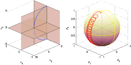
Figure 1: Example of numerical integration of the equation of motion for the case $\lambda=5$.  On the left the curve $\mathbf{\kappa}\left(s\right)$ is shown  and on the right the evolution of the polarization vector $\mathbf{p}\left(s\right)$ on the Bloch sphere is depicted.

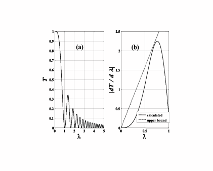
Figure 2: Calculated and upper bound of responsivity.  (a) Numerical calculation of $T$ vs. $\lambda$.  (b) Comparison between the calculater $\left|dT/d\lambda\right|$ and the upper bound given by Eq. 22.

The author thanks Avishai Eyal for very useful and stimulating discussions.

References

• (1) Mitchel Weissbluth, Photon-Atom Interaction (Academic Press, 1989).
• (2) E. Buks, ”Adiabatic Breakdown in a Fiber Ring Resonator,” J. Opt. Soc. Am. B (to be published) (arXiv: quant-ph/0412198).
• (3) M. V. Berry, ”Quantal Phase Factors Accompanying Adiabatic Changes ,” Proc. Roy. Soc. London A 392, 45 (1984).
• (4) A. B. Migdal, Qualitative methods in quantum theory (Benjamin, 1977).