Solid-state NMR three-qubit homonuclear system for quantum information processing: control and characterization

Abstract

A three-qubit ¹³C solid-state nuclear magnetic resonance (NMR) system for quantum information processing, based on the malonic acid molecule, is used to demonstrate high-fidelity universal quantum control via strongly modulating radio-frequency pulses. This control is achieved in the strong-coupling regime, in which the timescales of selective qubit addressing and of two-qubit interactions are comparable. State evolutions under the internal Hamiltonian in this regime are significantly more complex, in general, than those of typical liquid-state NMR systems. Moreover, the transformations generated by the strongly modulating pulses are shown to be robust against the types of ensemble inhomogeneity that dominate in the employed molecular crystal system. The secondary focus of the paper is upon detailed characterization of the malonic acid system. The internal Hamiltonian of the qubits is determined through spectral simulation. A pseudopure state preparation protocol is extended to make a precise measurement of the dephasing rate of a three-quantum coherence state under residual dipolar interactions. The spectrum of intermolecular ¹³C-¹³C dipolar fields in the crystal is simulated, and the results compared with single-quantum dephasing data obtained using appropriate refocusing sequences. We conclude that solid-state NMR systems tailored for quantum information processing have excellent potential for extending the investigations begun in liquid-state systems to greater numbers of qubits.

I Introduction

Quantum information processing (QIP) aims to achieve the ultimate in computational power from physical systems by exploiting their quantum nature Nielsen and Chuang (2000). Nuclear magnetic resonance (NMR)-based QIP has been successfully implemented in liquid-state ensemble systems of up to $7$ qubits Cory et al. (1998); Vandersypen et al. (2001); Yannoni et al. (1999); Cory et al. (2000); Knill et al. (2000); Das et al. (2004). Universal quantum control is achieved through application of external radio-frequency (RF) fields on or near resonance with spin transitions of a set of separately addressable, coupled spins. State initialization (to a fiducial state such as $|00..0\rangle$) is effectively achieved in these systems by the preparation of pseudopure states Cory et al. (1998); Knill et al. (1998a). Pseudopure states have recently been demonstrated in a 12-qubit liquid system Negrevergne et al. (2005) and in a 12-spin liquid-crystal system Lee and Khitrin (2005). A hallmark of control in liquid-state systems is a separation of timescales between (faster) qubit addressability and (slower) two-qubit coupling gates, typically by an order of magnitude or more Cory et al. (2000). For the homonuclear subsystems, this corresponds to the weak-coupling regime, in which the relative Zeeman shifts in the qubit Hamiltonian are significantly larger than the J-couplings Abragam (1961); Ernst and Bodenhausen (1987). In this regime, the evolution due to spin interactions is predominantly of the controlled-phase form. In this work, we examine NMR-based QIP implemented in a solid-state homonuclear system, in which the qubit Hamiltonian is no longer in the weak-coupling regime. A solid-state NMR architecture is attractive due to several key properties Cory et al. (2000): (1) nuclear spin states have been purified to near-unity polarizations in solids Abragam and Goldman (1982); (2) intrinsic decoherence times can be much longer, and two-qubit gate times much shorter, than those in the liquid state; (3) the qubit spins can be brought into well-controlled contact with a thermal-bath of bulk spins, enabling entropy-reducing operations such as algorithmic cooling Schulman and Vazirani (1990); Baugh et al. (2005) and quantum error correction Knill et al. (1998b); Laflamme et al. (1996) to be carried out. The system we will describe is specially tailored so that the ensemble description of the system is–to a good approximation–analogous to that of liquid-state NMR-QIP, and therefore the general aspects of control and measurement are the same Cory et al. (2000). A similar three qubit system using single-crystal glycine was first explored by Leskowitz et. al. Leskowitz et al. (2003), in which the homonuclear two-carbon system was approximately weakly-coupled. However, we will demonstrate that universal, coherent control can be implemented in the strong-coupling regime: the regime in which the timescales of qubit addressing and qubit coupling are comparable. In this regime, the transverse spin operator terms from qubit-qubit dipolar couplings are less suppressed by the relative Zeeman shifts. These residual ’flip-flop’ terms $\sigma^{j}_{+}\sigma^{k}_{-}+\sigma^{j}_{-}\sigma^{k}_{+}$ (where $\sigma_{\pm}=\sigma_{x}\pm i\sigma_{y}$ and $\{\sigma_{x},\sigma_{y}\}$ are Pauli matrices) render the state evolutions more complex, in general, than those of weakly-coupled spin systems. We show that strongly modulating pulses Fortunato et al. (2002) succeed in controlling the solid-state QIP system, with generality and with high-fidelity. Moreover, the pulses provide significant robustness for the desired transformations against the ensemble inhomogeneities that are typical of solid-state NMR systems. This latter property is of great importance to the practical application of quantum algorithms in such systems, and we present here a first step in its study. This control methodology is a key ingredient in the realization of solid-state NMR-QIP testbed devices, but could also extend to many other potential systems for quantum information processing. We remark that liquid-crystalline NMR-QIP implementations Das et al. (2004); Lee and Khitrin (2004) represent a coupling regime that is typically intermediate between the strong- and weak-coupling cases. Strongly modulating pulses would therefore also be an appropriate means for controlling such systems universally.
The secondary focus of this paper is to characterize, in detail, the employed three-qubit system based on the malonic acid molecule. This includes characterization of the dominant ensemble inhomogeneities arising both through linear and bi-linear terms in the Hamiltonian. In tailoring the present system, we have used dilution of the qubit molecules as a means for reaching an approximate ensemble description in which processor molecules are, ideally, non-interacting and reside in identical environments. However, the need for a macroscopic number of spins to generate observable NMR signals through the usual inductive detection both limits the degree of dilution and requires a macroscopic sample. The former results in perturbing intermolecular dipolar fields, and the latter typically yields significant distortions of the applied magnetic fields over the sample volume, namely, of the static magnetic field (due to susceptibility/shape effects) and of the RF amplitude (due to the RF coil geometry). In this paper, we address the robustness of strongly modulating pulse control to dispersion of Zeeman shifts and of RF amplitudes. We also characterize in detail the intermolecular dipolar environment in the present system, both theoretically and experimentally.
The paper is organized as follows: section II reviews strongly modulating RF pulses as a means of achieving universal quantum control, and numerical results for an example pulse are discussed; in section III, the dilute ¹³C malonic acid system is first characterized; section IV demonstrates the preparation of a pseudopure state (as a benchmark for control) and analyzes the results; section IV.3 treats an application of the pseudopure state protocol: precise measurement of the triple-quantum dipolar dephasing rate, and comparison to single-quantum dephasing rates; in section V, simulated and experimental data are presented that explore the effect of intermolecular dipolar couplings on qubit coherence times; in section V.2, a multiple-pulse refocusing sequence is used in order to compare appropriate experimental quantities with the intermolecular dipolar simulations, and as a first step in testing the attainability of long ensemble coherence times in this system; the overall results are discussed in section VI, in the context of assessing the future goals and potential of solid-state NMR-QIP.

II Universal Control: Strongly modulating pulses

Numerically optimized ’strongly modulating’ pulses were previously introduced as a means of implementing fast, high-fidelity unitary gate operations in the context of liquid-state NMR-QIP Fortunato et al. (2002). The aim is to construct an arbitrary modulated RF waveform that, when applied to the system, generates a desired effective Hamiltonian corresponding to a particular quantum gate. This is accomplished numerically by minimizing the distance between the actual and the desired unitary transformations using a simplex search algorithm. Gate fidelities are defined by the expression:

$$F=\sum_{\mu}p_{\mu}|Tr(U^{{\dagger}}_{des}U^{\mu}_{calc})/N|^{2}$$ (1)

where $N$ is the dimension of the Hilbert space, $U_{des}$ is the desired unitary and $U_{calc}$ is the unitary calculated for the evolution of the system under the modulated RF pulse. Here, $p_{\mu}$ is a normalized empirical distribution over an inhomogeneous parameter (or parameters) of the ensemble, typically the RF amplitude. The expression for $F$ corresponds to an average fidelity over all possible input states Fortunato et al. (2002). The number of parameters the algorithm must search over is made minimal by requiring the modulating waveform to consist of a series of constant amplitude and frequency periods, so that each period has a time-independent Hamiltonian in a particular rotating reference frame Fortunato et al. (2002). Modulation pulses with ideal (simulated) fidelities of order $F\sim 99\%$ are readily found for liquid-state NMR-QIP systems with up to 6 qubits Negrevergne et al. (2005); Fortunato et al. (2002).
It is observed empirically that good modulating pulse solutions tend to have the average RF amplitude $\nu_{RF}\sim|\mathcal{H}|$, where $|\mathcal{H}|$ is the magnitude of the internal qubit Hamiltonian. It is precisely this strong driving regime in which analytical techniques (e.g. perturbation theory) for calculating dynamics break down, yet the system generally has the broadest (and most rapid) access to the manifold of allowed states. It is also the regime in which all accessible spin transitions are excited, so that refocusing of unwanted interactions becomes possible, even to the extent that the dephasing effects of ensemble inhomogeneities may be partially suppressed Boulant et al. (2004); Rabitz (2002).
An example of a strongly modulating RF pulse is shown in Fig. 1. The pulse is tailored to generate a three-qubit controlled-(not$\otimes$not) gate in the strongly-coupled malonic acid system to be described in the next section. The average RF amplitude is $9.4$ kHz, whereas the magnitude of the internal ¹³C Hamiltonian (parameters listed in Table 1, next section) is $|\mathcal{H}|\simeq 7.3$ kHz. Part (c) of the figure demonstrates the robustness of the calculated unitary over the dominant inhomogeneous Hamiltonian parameters of the ensemble, namely, scaling of the RF amplitude and offset of the static field. This pulse was optimized over a 5-point probability distribution $p_{\mu}$ of RF amplitude scaling (corresponding to that measured in our RF coil), centered on unity, with standard deviation $\sigma(p_{\mu})\simeq 6\%$. The fact that the unitary fidelity is $>90\%$ over a $1$ kHz range of static field offset demonstrates the ability of the modulated pulse to effectively refocus evolution under Zeeman shift dispersion (no Zeeman distribution was used in the optimization). An ideal fidelity $\sim\!98\%$ was obtained here, however, even greater precision is likely required for successful general implementation of quantum algorithms. We consider this a first step that can be significantly improved upon in future work.
The strongly modulating pulse methodology generates fast pulses, relative to traditional selective pulse methods, to implement unitary gates. Although the example pulse of Fig. 1 has a duration $\simeq 700\mu$s, we have found pulse solutions for the same gate (fidelities $>90\%$) as short as $\simeq 450\mu$s. This compares well with the same gate carried out as two separate controlled-not gates implemented using standard low-amplitude selective $\pi/2$ pulses and $\pi/2$ controlled-phase evolutions; we estimate such a gate would require at least $\sim 1.25$ ms to implement. Optimal control theory has been used by other workers to design numerical procedures for constructing near time optimal state transformation pulses Khaneja et al. (2001).

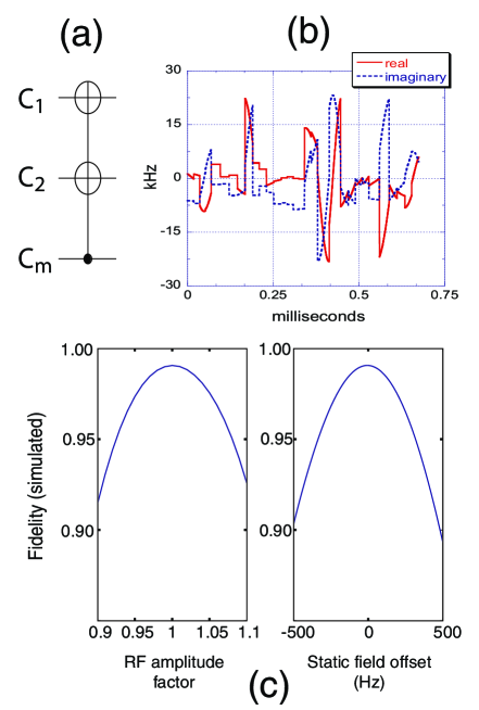
Figure 1: Example of a modulated RF pulse solution for generating a three-qubit gate in the malonic acid system. (a) quantum network representation of the gate, which is a controlled-(not$\otimes$not), with $C_{m}$ as the control bit and $C_{1}$ and $C_{2}$ as target bits. (b) the quadrature components of the RF modulation waveform, labelled ’real’ and ’imaginary’. (c) Simulated fidelity of the transformation as a function of (left) scaling of the RF amplitude and (right) offset of the static magnetic field.

III Characterization I: Ensemble Hamiltonian

III.1 Dilute 13C-labeled single-crystal malonic acid

The system under study is a single crystal of malonic acid grown from aqueous solution with a dilute fraction of fully ¹³C-labelled molecules. The main crystal used herein has dimensions of $4\!\times\!1.5\!\times\!1.5$ mm³ and a labelled molecule fraction of $3.2\%$ (a similar crystal with $1.6\%$ dilution was used in the experiments of section V.2). For the malonic acid molecule in the solid, the three carbon nuclei have distinct anisotropic chemical shielding tensors so that when placed in a large static magnetic field, crystal orientations can be found for which each carbon is separately addressable in frequency. Protons, of which there are four per molecule (and are $100\%$ abundant in the crystal), can be used to cross-polarize the carbon spins, and are otherwise decoupled from the ¹³C system. Figure  2 shows the malonic acid unit cell as determined by x-ray diffraction Jagannathan et al. (1994). The space group is P-1 so that the two molecules in the unit cell are related by inversion symmetry, and are therefore magnetically equivalent. The crystal orientation is chosen to maximize the intramolecular ¹³C-¹³C dipolar couplings and the relative ¹³C Zeeman shifts. The full spin Hamiltonian of the system is

$$\mathcal{H}(t)=\mathcal{H}_{C}+\mathcal{H}_{H}+\mathcal{H}_{CH}+\mathcal{H}_{RF}(t),$$ (2)

where $\mathcal{H}_{C}$ and $\mathcal{H}_{H}$ are the ¹³C and ¹H Hamiltonians, $\mathcal{H}_{CH}$ is the interspecies coupling Hamiltonian, and $\mathcal{H}_{RF}(t)$ is the time-dependent Hamiltonian of the external radio-frequency field. In many experiments, $\mathcal{H}_{RF}(t)$ includes a strong field resonant with the ¹H spins so that $\mathcal{H}_{CH}$ is effectively removed from the Hamiltonian. The ¹³C Hamiltonian can be decomposed as

$$\mathcal{H}_{C}=\mathcal{H}_{CZ}+\mathcal{H}^{intra}_{CD}+\mathcal{H}^{inter}_{CD},$$ (3)

where the terms on the right side, from left to right, are the Zeeman, the intramolecular dipolar, and the intermolecular dipolar terms. The Zeeman and intramolecular dipolar terms dominate the natural ¹³C Hamiltonian in the dilute ¹³C crystal, and will be used (along with the RF) in the construction of quantum gates. The intermolecular couplings act as perturbations on these terms, and their effects will be examined in section V. Denoting single-spin Pauli matrices as $X=\sigma_{x}\quad,Y=\sigma_{y}\quad,Z=\sigma_{z}$, the Zeeman and intramolecular dipolar terms may be expressed as

$$\mathcal{H}_{CZ}=\sum^{3}_{j=1}\frac{\nu_{j}}{2}Z^{j}$$ (4)

$$\mathcal{H}^{intra}_{CD}=\sum_{m<n\leq 3}\frac{d_{mn}}{4}(2Z^{m}Z^{n}-Y^{m}Y^{n}-X^{m}X^{n}),$$ (5)

where $\nu_{j}$ are the rotating-frame Zeeman frequencies and $d_{mn}$ are the dipolar coupling strengths. Table I lists these parameters, as obtained from fitting the ¹³C spectrum of Figure 3, for the crystal orientation used throughout. It also lists the free-induction dephasing times, $T_{2}^{*}$; the corresponding rates $(T_{2}^{*})^{-1}$ provide a measure of the degree of ensemble inhomogeneity. It will be seen in section V. that the dominant contribution to these rates is Zeeman shift dispersion.

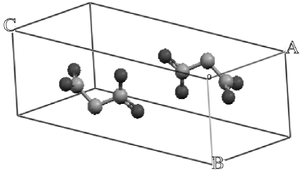
Figure 2: Unit cell of malonic acid, with crystal axes indicated. The two molecules are related by inversion symmetry, and are therefore magnetically equivalent (P-1 space group). The light (dark) atoms are carbon (oxygen), and the hydrogen atoms are not shown. $\vec{A}=5.156$Å, $\vec{B}=5.341$Å  and $\vec{C}=8.407$ÅJagannathan et al. (1994).

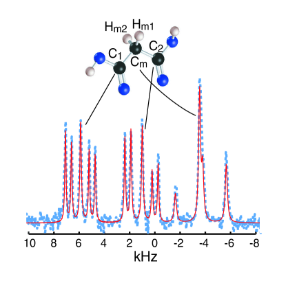
Figure 3: ¹³C-NMR spectrum (dotted line) and spectral fitting results (solid line) for $3.2\%$ ¹³C-labelled malonic acid in the crystal orientation used throughout. The fitting procedure adjusts the simulated Hamiltonian to match the spectrum, and uses Lorentzian line broadening to fit the $(T_{2}^{*})^{-1}$ depashing rates. Proton decoupling was applied using a TPPM sequence Bennett et al. (1995) at an RF power of $250$ kHz. Note the most intense peaks, in the center of each multiplet, correspond to the natural abundance ($1.1\%$) ¹³C. The uneven heights of the labelled-molecule peaks indicate that the relative Zeeman shifts are insufficient to fully truncate the strong form of the intramolecular dipolar couplings; hence, the eigenstates of the system are near, but not equal to, the usual computational basis states.

Table 1: Zeeman shifts and intramolecular dipolar couplings of the ¹³C Hamiltonian, columns 1-3 from left; dipolar couplings involving the methylene protons, columns 4-5; ¹³C free-induction dephasing times ($T_{2}^{*}$) and spin-lattice relaxation times ($T_{1}$). Values in columns 1-5 are in kHz.

	$C_{1}$	$C_{2}$	$C_{m}$	$H_{m1}$	$H_{m2}$	$T_{2}^{*}$(ms)	$T_{1}$(s)
$C_{1}$	$5.893$	$0.227$	$0.935$	$-1.5$	$2.0$	$2.4$	$160$
$C_{2}$		$1.057$	$1.070$	$1.4$	$1.0$	$2.0$	$325$
$C_{m}$			$-3.445$	$-18.7$	$-0.9$	$1.5$	$315$

III.2 Experimental setup

All experiments were carried out at room temperature on a Bruker Avance NMR spectrometer operating at a field of $7.1$ T, and home-built dual-channel RF probehead. The sample coil had an inner diameter of $3$ mm, and the typical $\pi/2$ ’hard’ pulse lengths were $1.25\mu$s and $0.75\mu$s for carbon and hydrogen, respectively.

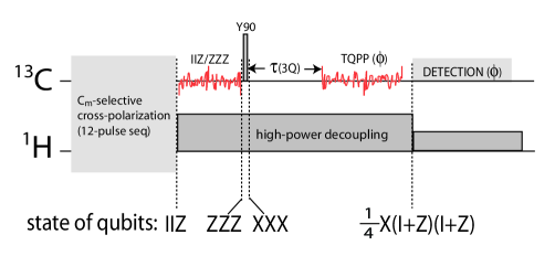
Figure 4: Schematic pulse sequence for pseudopure state preparation using strongly modulating pulses. The states of the qubits are indicated in product operator format after each transformation. The state ${\mathchoice{\rm 1\mskip-4.0mul}{\rm 1\mskip-4.0mul}{\rm 1\mskip-4.5mul}{\rm 1\mskip-5.0mul}}^{1}{\mathchoice{\rm 1\mskip-4.0mul}{\rm 1\mskip-4.0mul}{\rm 1\mskip-4.5mul}{\rm 1\mskip-5.0mul}}^{2}Z^{m}$ is denoted as ’IIZ’, for example. Strongly modulating pulses are represented by waveforms labelled ’IIZ/ZZZ’ and ’TQPP’, whose durations are $0.54$ ms and $1.10$ ms, respectively. A collective $\pi/2$ rotation about the rotating-frame $\hat{y}$-axis is labelled ’Y90’. The angle $\phi$ represents a six-fold phase-shifting of the RF to filter out all coherences except the 3Q coherence. $\tau(3Q)$ indicates a variable delay subsequent to the creation of the 3Q state that is used to measure that state’s decay.

IV Pseudopure state

IV.1 Preparation method

A labelled pseudopure state Cory et al. (1998); Knill et al. (1998a) can be prepared in this system using a combination of tailored RF pulses and RF phase cycling (temporal averaging). A schematic of the pulse sequence is shown in Figure 4. The first step is a selective transfer of ¹H polarization to the methylene carbon $C_{m}$, utilizing the ¹H/¹³C coupling Hamiltonian $\mathcal{H}_{CH}$. While it is not necessary for this protocol to begin with a selective transfer, we demonstrate it here because it may be used in other algorithms for controlled, selective coupling of the qubit system to the bulk ¹H system (which can be considered as a thermal-bath of spin polarization). To accomplish the transfer, a pulse sequence is applied on both ¹H and ¹³C channels synchronously, which, by design, effectively removes $\mathcal{H}_{C}+\mathcal{H}_{H}$ from the ensemble Hamiltonian Cory et al. (1990); Haeberlen (1976). In such sequences, homonuclear dipolar terms are refocussed by toggling the interaction-frame Hamiltonian along the rotating-frame $\hat{x}$, $\hat{y}$ and $\hat{z}$ directions, spending equal time along each axis. Therefore, the dual sequence creates (to lowest order in the Magnus expansion of the average Hamiltonian Haeberlen (1976)) an effective ¹H-¹³C exchange Hamiltonian

$$\mathcal{H}_{\text{eff}}=\sum_{j\in C,k\in H}\frac{d_{jk}}{3}\frac{(Z^{j}Z^{k}+Y^{j}Y^{k}+X^{j}X^{k})}{2},$$ (6)

where $d_{jk}$ are pairwise ¹H-¹³C dipolar coupling constants, and the indices $j,k$ run over all ¹³C,¹H spins, respectively. In the special case that there is only one coupled carbon/proton pair with a coupling of $d_{CH}$, application of the sequence for a time $\tau=3/(4d_{CH})$ will result in a state exchange between the two nuclei. Since this is approximately the case for the strong methylene ¹H-¹³C coupling in our oriented malonic acid system (see Table I), we may implement a nearly selective polarization transfer to $C_{m}$ of magnitude $P\simeq P_{H}=3.98P_{C}$ ($P_{C}$ and $P_{H}$ are the thermal equilibrium carbon and proton polarizations, respectively). Furthermore, this selective transfer removes a very small amount of polarization from the ¹H bath, since only the methylene protons on a dilute fraction of ¹³C-labelled molecules lose their polarization. The remaining bulk ¹H polarization is preserved since the sequence is effectively a time-suspension sequence for the bulk spins. In our system, a selective polarization transfer of about $83\%$ of $P_{H}$ to $C_{m}$ was achieved with a 12-pulse subsequence of the Cory 48-pulse sequence Cory et al. (1990); the duration of the 12-pulse sequence was $40\mu$s for maximum transfer. The thermal equilibrium ¹³C polarization can be removed prior to such a transfer by rotating the equilibrium ¹³C state ($\propto Z$) into the transverse ($\hat{x}-\hat{y}$) plane and allowing it to dephase under local ¹H dipolar fields.
Product operator terms denoting qubit states are ordered as $C_{1}\otimes C_{2}\otimes C_{m}$; for example, the symbol ${\mathchoice{\rm 1\mskip-4.0mul}{\rm 1\mskip-4.0mul}{\rm 1\mskip-4.5mul}{\rm 1\mskip-5.0mul}}XZ$ corresponds to the state ${\mathchoice{\rm 1\mskip-4.0mul}{\rm 1\mskip-4.0mul}{\rm 1\mskip-4.5mul}{\rm 1\mskip-5.0mul}}^{1}\otimes X^{2}\otimes Z^{m}$. Also, single-spin terms such as $X^{1}\otimes{\mathchoice{\rm 1\mskip-4.0mul}{\rm 1\mskip-4.0mul}{\rm 1\mskip-4.5mul}{\rm 1\mskip-5.0mul}}^{2}\otimes{\mathchoice{\rm 1\mskip-4.0mul}{\rm 1\mskip-4.0mul}{\rm 1\mskip-4.5mul}{\rm 1\mskip-5.0mul}}^{m}$ are sometimes abbreviated as $X^{1}$, for example. The polarization transfer is followed by a ¹³C modulating RF pulse that transforms the state ${\mathchoice{\rm 1\mskip-4.0mul}{\rm 1\mskip-4.0mul}{\rm 1\mskip-4.5mul}{\rm 1\mskip-5.0mul}}{\mathchoice{\rm 1\mskip-4.0mul}{\rm 1\mskip-4.0mul}{\rm 1\mskip-4.5mul}{\rm 1\mskip-5.0mul}}Z$ to $ZZZ$, and then a collective $\pi/2$ pulse that rotates this to $XXX$. In addition to single-quantum (1Q) terms, this state contains the triple-quantum (3Q) coherence $\sigma_{+}\sigma_{+}\sigma_{+}+\sigma_{-}\sigma_{-}\sigma_{-}$, where $\sigma_{+}=X+iY$ and $\sigma_{-}=X-iY$. A subsequent modulating pulse (denoted ’TQPP’ for ’triple-quantum to pseudopure’) transforms the 3Q coherence into the labelled pseudopure state $X({\mathchoice{\rm 1\mskip-4.0mul}{\rm 1\mskip-4.0mul}{\rm 1\mskip-4.5mul}{\rm 1\mskip-5.0mul}}+Z)({\mathchoice{\rm 1\mskip-4.0mul}{\rm 1\mskip-4.0mul}{\rm 1\mskip-4.5mul}{\rm 1\mskip-5.0mul}}+Z)$. This state is observable as a single NMR transition of $C_{1}$ . In order to cancel all other signals arising from the 1Q terms in the state $XXX$, phase cycling is used which exploits the $n$-proportional phase acquisition of an $n$-quantum state under $\hat{z}$-axis rotation. Choosing desired coherence pathways using phase cycling is widely practiced in modern NMR spectroscopy Ernst and Bodenhausen (1987). By shifting the phase of the RF by $\phi$ during the TQPP pulse, the unitary transformation generated by the pulse is rotated by $\phi$ about $Z^{\prime}=Z^{1}+Z^{2}+Z^{m}$:

$$U_{tqpp}(\phi)=R_{z}^{\phi}U_{tqpp}R_{z}^{-\phi},$$ (7)

where $R_{z}^{\phi}\equiv e^{-i(Z^{\prime})\phi/2}$. Note this is only true since the internal Hamiltonian of the system commutes with $Z^{\prime}$, hence a $\hat{z}$-axis rotation can be accomplished by acting only on the phase of the RF pulse. We may decompose the state prior to the TQPP pulse into 3Q and 1Q terms, e.g. $XXX=\rho_{\pm 3Q}+\rho_{\pm 1Q}$. The final density matrix is calculated as

$$\rho_{f}(\phi)=R_{z}^{\phi}U_{tqpp}R_{z}^{-\phi}(\rho_{\pm 3Q}+\rho_{\pm 1Q})R_{z}^{\phi}U^{{\dagger}}_{tqpp}R_{z}^{-\phi}$$

$$=R_{z}^{\phi}((e^{-3i\phi}\sigma_{+}+e^{3i\phi}\sigma_{-})({\mathchoice{\rm 1\mskip-4.0mul}{\rm 1\mskip-4.0mul}{\rm 1\mskip-4.5mul}{\rm 1\mskip-5.0mul}}+Z)({\mathchoice{\rm 1\mskip-4.0mul}{\rm 1\mskip-4.0mul}{\rm 1\mskip-4.5mul}{\rm 1\mskip-5.0mul}}+Z)/8+e^{\mp i\phi}\rho^{\prime})R_{z}^{-\phi},$$ (8)

where $\rho^{\prime}=U_{tqpp}(\rho_{\pm 1Q})U^{{\dagger}}_{tqpp}$. Incrementing $\phi$ in units of $\frac{\pi}{3}$ for $6$ scans, alternately adding and subtracting, adds constructively the 3Q terms while cancelling the 1Q terms, since

$$\sum_{k=1}^{6}(-1)^{k-1}e^{\pm nik\frac{\pi}{3}}=6\cdot\delta(n-3m),$$ (9)

where $m$ is an odd integer, and here $m=1$ since $n\leq 3$. The remaining $\hat{z}$-rotation $R_{z}^{\phi}$ is undone by incrementing the phase of the receiver along with that of the TQPP modulating RF pulse. The labelled pseudopure state is thus obtained as

$$\frac{1}{6}\sum_{k=1}^{6}(-1)^{k-1}R_{z}^{-k\pi/3}\rho_{f}(k\pi/3)R_{z}^{k\pi/3}=X({\mathchoice{\rm 1\mskip-4.0mul}{\rm 1\mskip-4.0mul}{\rm 1\mskip-4.5mul}{\rm 1\mskip-5.0mul}}+Z)({\mathchoice{\rm 1\mskip-4.0mul}{\rm 1\mskip-4.0mul}{\rm 1\mskip-4.5mul}{\rm 1\mskip-5.0mul}}+Z)/4.$$ (10)

The amount of signal contained in the resulting pseudopure state is $1/4$ that of the input state, equal to the proportion of the 3Q part of the state $XXX$.

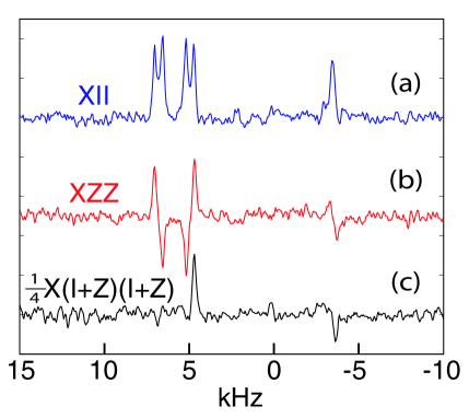
Figure 5: Experimental results for the pseudopure state protocol. (a) readout of the state ${\mathchoice{\rm 1\mskip-4.0mul}{\rm 1\mskip-4.0mul}{\rm 1\mskip-4.5mul}{\rm 1\mskip-5.0mul}}{\mathchoice{\rm 1\mskip-4.0mul}{\rm 1\mskip-4.0mul}{\rm 1\mskip-4.5mul}{\rm 1\mskip-5.0mul}}Z$ just after the selective polarization transfer, with readout consisting of a swap from $C_{m}$ to $C_{1}$ and collective $\pi/2$ pulse about the $\hat{y}$-axis to produce $X{\mathchoice{\rm 1\mskip-4.0mul}{\rm 1\mskip-4.0mul}{\rm 1\mskip-4.5mul}{\rm 1\mskip-5.0mul}}{\mathchoice{\rm 1\mskip-4.0mul}{\rm 1\mskip-4.0mul}{\rm 1\mskip-4.5mul}{\rm 1\mskip-5.0mul}}$; (b) readout of the state $ZZZ$ by a $C_{1}$-selective $\pi/2$ rotation to produce the observable state $XZZ$; (c) the labelled pseudopure state yields a single absorption peak from the $C_{1}$ multiplet. Fitting the data by spectral simulation indicates a protocol state-correlation of $87\%\pm 5\%$, using spectrum (a) as a reference.

IV.2 Pseudopure state results

Results for the pseudopure state protocol of Fig. 4 are shown in Fig. 5. It shows (a) readout of the state ${\mathchoice{\rm 1\mskip-4.0mul}{\rm 1\mskip-4.0mul}{\rm 1\mskip-4.5mul}{\rm 1\mskip-5.0mul}}{\mathchoice{\rm 1\mskip-4.0mul}{\rm 1\mskip-4.0mul}{\rm 1\mskip-4.5mul}{\rm 1\mskip-5.0mul}}Z$ just after the selective polarization transfer, with readout consisting of a state-swap from $C_{m}$ to $C_{1}$ followed by a collective $\pi/2$ pulse to produce $X{\mathchoice{\rm 1\mskip-4.0mul}{\rm 1\mskip-4.0mul}{\rm 1\mskip-4.5mul}{\rm 1\mskip-5.0mul}}{\mathchoice{\rm 1\mskip-4.0mul}{\rm 1\mskip-4.0mul}{\rm 1\mskip-4.5mul}{\rm 1\mskip-5.0mul}}$; (b) readout of the state $ZZZ$ by a $C_{1}$-selective $\pi/2$ rotation to produce the observable state $XZZ$; (c) the labelled pseudopure state yields a single absorption peak from the $C_{1}$ multiplet. Using the spectrum (a) as reference, the state-correlation of the pseudopure state protocol, determined by spectral fitting, is $87\%\pm 5\%$. Similarly, the state-correlation of the TQPP pulse, using the $XZZ$ spectrum (b) as a reference, is $97\%\pm 5\%$. These results serve as a benchmark for quantum control in the strongly-coupled dilute molecular crystal system. They suggest that dephasing due to Zeeman shift dispersion is largely suppressed by these pulses, since the average free-induction dephasing time of the qubits is $T^{\ast}_{2}\simeq 2$ ms, and the total duration of the two modulating pulses, $\simeq 1.6$ ms, is a large fraction of that time.

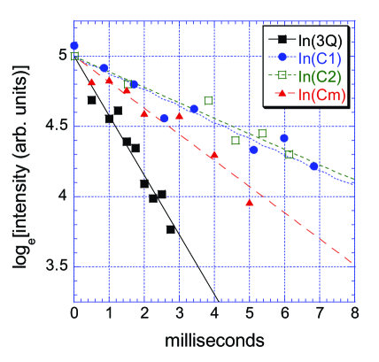
Figure 6: Triple-quantum (3Q) and single-quantum dephasing data, plotted as the natural log of the signal intensity. Exponential fits indicate decay time constants (in milliseconds) of [$2.37\,(3Q),\,5.37\,(C_{m}),\,9.07\,(C_{2}),\,8.66\,(C_{1})$].

IV.3 Dipolar dephasing of triple-quantum coherence

Dephasing of the 3Q coherence state $\sigma_{+}\sigma_{+}\sigma_{+}+\sigma_{-}\sigma_{-}\sigma_{-}$ was measured by inserting a variable time delay $\tau(3Q)$ following the ’Y90’ pulse in Fig. 4. A collective $\pi$ pulse was also inserted in the center of $\tau(3Q)$ to refocus Zeeman Hamiltonian terms (Hahn echo), so that the measured dephasing rate reflects only the perturbing dipolar fields experienced by the nuclei. This 3Q state is significant from a QIP perspective since it consists of the two most fragile density matrix elements in the three-qubit system, the extreme off-diagonal elements that are contained in the so-called ”cat-state” $|000\rangle+|111\rangle$. The resulting signal decay is shown in Fig. 6 along with the 1Q dephasing data for each qubit, also measured via Hahn echo. The 1Q decay data were measured by first preparing the states $X^{1}$, $X^{2}$ and $X^{m}$, and using the pair of outer spectral peaks from each spin multiplet to gauge the signal, observing only at delays corresponding to multiples of the dipolar oscillation periods of these peaks. Exponential fits yield decay time constants (in milliseconds) [$2.37\,(3Q),\,5.37\,(C_{m}),\,9.07\,(C_{2}),\,8.66\,(C_{1})$], with experimental uncertainty $\simeq\pm 11\%$ for each value. Within error, the observed 3Q dephasing rate is equal to the sum of the three 1Q rates. In the next section, we will see that intermolecular ¹³C-¹³C dipolar fields lead to an approximately Lorentzian frequency broadening of the 1Q transitions. In this regime, the 1Q dephasing appears as a Markovian process, and therefore we do not expect the 3Q rate to carry any information about correlations in the 3Q dephasing. The fact that the observed 3Q rate is the sum of the 1Q rates is consistent with this picture.
Finally, we remark that the faster 1Q dephasing of the methylene carbon $C_{m}$ evident in Fig. 6 is probably due to a residual interaction with its neighboring proton, as the methylene proton pair are strongly coupled ($22$ kHz) which makes it difficult to remove the $19$ kHz $C_{m}$-$H_{m1}$ coupling under the standard TPPM decoupling used here. This effect is directly evident in the data presented in section V.2 (note, however, the data in section V.2 was obtained in a different sample at a slightly different orientation with respect to the external field).

V Characterization II: Intermolecular dipolar fields

V.1 Modelling intermolecular dipolar dephasing

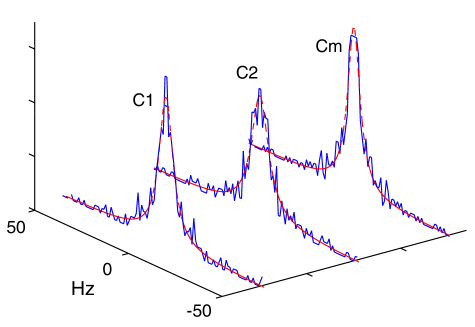
Figure 7: Simulation of line-shapes resulting from intermolecular dipolar couplings in $1.9\%$ molecular dilution ¹³C malonic acid. The simulated data (solid lines) are shown with Lorentzian fits (dashed lines). The resulting linewidths (FWHM) for $C_{1}$, $C_{2}$ and $C_{m}$ are $9$, $11$ and $8$ Hz respectively. Correcting for the larger spin concentration due to presence of natural abundance spins, the linewidths should be approximately $60\%$ broader.

We now turn our attention to characterizing ¹³C-¹³C intermolecular dipolar interactions in the dilute malonic acid system. The general Hamiltonian of the system is

$$\mathcal{H}=\sum_{j<k}d_{jk}h_{jk}+\sum_{l}\frac{\nu_{l}}{2}Z^{l},$$ (11)

where $d_{jk}=d_{jk}(r_{jk},\theta_{jk})$ are the intermolecular dipolar coupling constants that depend on the internuclear vector of length $r_{jk}$ and orientation $\theta_{jk}$ (with respect to the external field), $h_{jk}$ is the spin-operator of the form of the dipolar coupling as in Eq. 5, and $\nu_{l}$ are the chemical shifts. Taking a reference spin $l=1$ to be a $C_{1}$ spin, we may transform to the $C_{1}$ rotating frame by setting all $\nu_{l}=0$ for $l\in\{C_{1}\}$, and setting $\nu_{l^{\prime}}$ to the correct offset frequencies for $l^{\prime}\in\{C_{2},C_{3}\}$, respectively. The latter offset frequencies $\nu_{l^{\prime}}$ are on the order of a few kHz (see Table 1), whereas the intermolecular couplings $d_{jk}$ are much weaker ($<\!100$ Hz) due to the $r_{jk}^{-3}$ scaling of the dipolar interaction. We may therefore truncate couplings between unlike spins $C_{\alpha}$-$C_{\beta}$ to the heteronuclear form, and rewrite the dipolar terms as an ensemble of reference-spin Hamiltonians (e.g. for the $C_{1}$ reference ensemble):

$$\mathcal{H}_{dip} =\sum_{j,k}\mathcal{H}^{jk}_{dip};$$

$$\mathcal{H}^{jk}_{dip} =\frac{d_{\alpha jk}}{2}Z^{1j}Z^{\alpha jk}+\frac{d_{\beta jk}}{2}Z^{1j}Z^{\beta jk}$$

$$+\frac{d_{\gamma jk}}{4}(2Z^{1j}Z^{\gamma jk}-X^{1j}X^{\gamma jk}-Y^{1j}Y^{\gamma jk}),$$ (12)

where $j$ indicates a particular reference spin from the $C_{1}$ ensemble, and $k$ denotes the set of spin-labelled molecules that interact with the $j^{th}$ reference spin. $\alpha$, $\beta$ and $\gamma$ indicate spins belonging to the $C_{m}$, $C_{2}$ and $C_{1}$ ensembles, respectively. Note that the above Hamiltonian does not include all dipolar terms in Eq. 11, since it only includes strong-coupling terms between $C_{1}$ spins, and so implicitly neglects much of the spin-diffusion dynamics. We wish to make an estimate of the dephasing rate (i.e. line broadening) of the reference spins due to this ensemble interaction Hamiltonian (see Norberg and Lowe (1957) for seminal work along these lines). An approximate result can be obtained in the spin-dilute regime by assuming that the reference spin only interacts with one nearby spin-labelled molecule, so that there is only one $k$ value and $\mathcal{H}^{jk}_{dip}=\mathcal{H}^{j}_{dip}$.
Under this restricted model, we will now describe the dephasing process in terms of the quantum evolution of the ensemble. The system consists of the reference spin, denoted $\xi$, and the three interacting spins $\alpha,\beta,\gamma$. The initial state is described by the density matrix $\rho_{\xi}\otimes\rho_{\alpha\beta\gamma}$, where at thermal equilibrium $\rho_{\alpha\beta\gamma}={\mathchoice{\rm 1\mskip-4.0mul}{\rm 1\mskip-4.0mul}{\rm 1\mskip-4.5mul}{\rm 1\mskip-5.0mul}}$ is appropriate for high-temperature NMR. The unitary operator acting on the $j^{th}$ ensemble member of the system at time $t$ is

$$U_{j}(t)=e^{-i\mathcal{H}^{j}_{dip}2\pi t},$$ (13)

The operators that act on the reduced density matrix $\rho_{\xi}$ of the reference spin, i.e. the Kraus operators, are derived from the submatrices of $U$:

$$U_{mn}=\langle\psi^{m}_{\alpha\beta\gamma}|U|\psi^{n}_{\alpha\beta\gamma}\rangle,$$ (14)

where $|\psi^{n}_{\alpha\beta\gamma}\rangle$ is the $n^{th}$ eigenvector of the $\alpha,\beta,\gamma$ system in some eigenbasis. Since $\rho_{\alpha\beta\gamma}={\mathchoice{\rm 1\mskip-4.0mul}{\rm 1\mskip-4.0mul}{\rm 1\mskip-4.5mul}{\rm 1\mskip-5.0mul}}$, the Kraus operators $A_{m}$ are obtained by summing with equal weights over the basis vectors:

$$A_{m}=2^{-q}\sum^{2^{q}}_{n=1}U_{mn},$$ (15)

where the number of interacting spins is $q=3$ in our case. In the standard computational basis, $|\psi^{n}_{\alpha\beta\gamma}\rangle\in\{|000\rangle,|001\rangle,...,|111\rangle\}$, we obtain for $U_{j}(t)$ operators of the form (subscripts $k,l,m\in\{0,1\}$ denote the basis vector of the $\alpha,\beta,\gamma$ system):

$$A^{j}_{klm}(t)=\frac{1}{8}\times$$

$$[|0\rangle\langle 0|e^{i\frac{\theta_{\alpha j}}{2}(-1)^{k}+i\frac{\theta_{\beta j}}{2}(-1)^{l}+i\frac{\theta_{\gamma j}}{2}(-1)^{m}}(\frac{e^{i\frac{\theta_{\gamma j}}{2}\delta_{m1}}+e^{-i\frac{\theta_{\gamma j}}{2}\delta_{m1}}}{2})+|1\rangle\langle 1|e^{-i\frac{\theta_{\alpha j}}{2}(-1)^{k}-i\frac{\theta_{\beta j}}{2}(-1)^{l}-i\frac{\theta_{\gamma j}}{2}(-1)^{m}}(\frac{e^{i\frac{\theta_{\gamma j}}{2}\delta_{m0}}+e^{-i\frac{\theta_{\gamma j}}{2}\delta_{m0}}}{2})$$

$$+|1\rangle\langle 0|\delta_{m0}e^{i\frac{\theta_{\alpha j}}{2}(-1)^{k}+i\frac{\theta_{\beta j}}{2}(-1)^{l}-i\frac{\theta_{\gamma j}}{2}}(\frac{-e^{i\frac{\theta_{\gamma j}}{2}}+e^{-i\frac{\theta_{\gamma j}}{2}}}{2})+|0\rangle\langle 1|\delta_{m1}e^{i\frac{\theta_{\alpha j}}{2}(-1)^{k}+i\frac{\theta_{\beta j}}{2}(-1)^{l}-i\frac{\theta_{\gamma j}}{2}}(\frac{-e^{i\frac{\theta_{\gamma j}}{2}}+e^{-i\frac{\theta_{\gamma j}}{2}}}{2})]$$ (16)

where $\theta_{\eta j}=2\pi td_{\eta j}$, and $\delta_{ab}$ is the Kronecker delta.
To study dephasing behavior, we apply the eight Kraus operators $A^{j}_{klm}(t)$ to the reference spin state $\rho_{\xi}=X=|0\rangle\langle 1|+|1\rangle\langle 0|$, obtaining

$$\rho^{j}_{\xi}=\sum_{klm}A^{j}_{klm}\rho_{\xi}(A^{j}_{klm})^{{\dagger}}=\sum_{klm}(a^{j}_{klm}|0\rangle\langle 1|+b^{j}_{klm}|1\rangle\langle 0|),$$ (17)

where

$$a^{j}_{klm}=\frac{1}{8}\times$$

$$e^{i\theta_{\alpha j}(-1)^{k}+i\theta_{\beta j}(-1)^{l}}\frac{e^{i\theta_{\gamma j}((-1)^{m}+1/2)}+e^{i\theta_{\gamma j}((-1)^{m}-1/2)}}{2}$$ (18)

and

$$b^{j}_{klm}=\frac{1}{8}\times$$

$$e^{-i\theta_{\alpha j}(-1)^{k}-i\theta_{\beta j}(-1)^{l}}\frac{e^{-i\theta_{\gamma j}((-1)^{m}-1/2)}+e^{-i\theta_{\gamma j}((-1)^{m}+1/2)}}{2}$$ (19)

Inspection of equations 18 and 19 shows that $\rho^{j}_{\xi}$ gains phases $\pm\theta_{\alpha j}\pm\theta_{\beta j}\pm\theta_{\gamma j}/2$ and $\pm\theta_{\alpha j}\pm\theta_{\beta j}\pm 3\theta_{\gamma j}/2$ characteristic of generic binomial distributions. Averaging over the ensemble of Hamiltonians $\mathcal{H}^{j}_{dip}$, we obtain $\rho_{\xi}(t)=\sum^{N}_{j=1}\rho^{j}_{\xi}(t)/N$. Defining a correlation function $F_{x}(t)=Tr(\rho_{\xi}(t)\cdot X)$, its frequency spectrum is given by the Fourier transformation $\hat{F}_{x}(\omega)=\int^{\infty}_{-\infty}e^{i\omega t}F_{x}(t)$. Equations 18 and 19 make clear that $\hat{F}_{x}(\omega)$ will simply reflect the ensemble distribution of the intermolecular coupling constants leading to frequencies $2\pi\{\pm d_{\alpha j}\pm d_{\beta j}\pm d_{\gamma j}/2\}$ and $2\pi\{\pm d_{\alpha j}\pm d_{\beta j}\pm 3d_{\gamma j}/2\}$.
To make a concrete calculation of the distribution of coupling constants $d_{\eta j}$, let us further assume that the interacting molecule lies within the first shell of 26 neighboring unit cells. Each unit cell contains two (magnetically equivalent) molecules, giving a total of $156$ atomic sites ($159$ after adding the 3 atomic sites of the unit cell neighbor to the reference molecule). We calculated the coupling constants to each of these sites using the Cartesian atomic coordinates obtained by x-ray diffraction Jagannathan et al. (1994) and the unit cell vectors $(\vec{A},\vec{B},\vec{C})$ (see Fig. 2). The couplings are explicitly of the form:

$$d_{k}(r_{k},\theta_{k})=\gamma^{2}_{C}\hbar\frac{1-3cos^{2}(\theta_{k})}{2r_{k}^{3}},$$ (20)

where $\gamma_{C}$ is the gyromagnetic ratio of ¹³C, $r_{k}$ is the length of the internuclear vector connecting spin $k$ to the reference spin, and $\theta_{k}$ is the angle between this vector and the external magnetic field direction. Note that since there are $53$ molecular sites we are considering, the random occupation of one site corresponds to a labelled-molecule concentration of $\frac{1}{53}=1.9\%$, which is in the range of our sample concentrations. Following the discussion above, we constructed frequency histograms by averaging the spectral frequencies $2\pi\{\pm d_{\alpha j}\pm d_{\beta j}\pm 3d_{\gamma j}/2\}$ over the distribution of coupling constants to the 53 molecular sites. The same procedure was carried out for $C_{1}$, $C_{2}$ and $C_{m}$ as reference spins. Figure 7 shows the resulting histograms calculated for the crystal orientation used throughout. Lorentzian functions provide good fits for the purpose of determining the spectral linewidths, as expected for a dilute spin system Abragam (1961).
The simulated spectra of figure 7 correspond to the expected indirect-dimension line-shapes that would result in a two-dimensional NMR experiment under a Hahn echo sequence Ernst and Bodenhausen (1987). The fits yield full-width half-maximum (FWHM) linewidths $\Delta\nu\sim 10$ Hz. The presence of single ¹³C spins due to natural abundance ($1.1\%$ atomic concentration) adds to the total spin concentration. This broadens the linewidth estimate by a factor $\simeq\frac{\eta+1.1\%}{1.9\%}$ for a dilute labelled-molecule percentage $\eta<10\%$, since linewidth is approximately linear in spin concentration in this dilute regime Abragam (1961). To account for interactions with molecules beyond the first neighboring unit cells in this static broadening picture (i.e. ignoring spin-diffusion dynamics), we can make a crude shell-model approximation. The broadening from the $n$ spins in a spherical shell of radius $R$, $n(R)\propto R^{2}$, will go as $R^{-3}\sqrt{n(R)}\propto R^{-2}$. This is true since the width (i.e. standard deviation) of a binomial distribution scales as $\sqrt{n}$ and the dipolar interaction scales as $R^{-3}$. Hence, the linewidths should be larger by a factor $\sum^{\infty}_{k=1}k^{-2}=\pi^{2}/6$. The results, adjusted for $\eta=1.6\%$, are summarized in Table 2 along with experimental data obtained in a $1.6\%$ labelled-molecule dilution crystal. The experimental values indicate effective Lorentzian linewidths of the natural abundance ¹³C spins measured via Hahn echo, and by a multiple-pulse sequence consisting of the MREV-8 dipolar refocusing sequence Haeberlen (1976) in combination with the Hahn echo (detailed in the following section). In the table, ’Simulation II’ refers to the aforementioned spectral simulations. These values should correspond to the Hahn echo experimental data. ’Simulation I’ refers to simulations in which like-spin $C_{\alpha}$-$C_{\alpha}$ couplings were omitted. These values should correspond roughly with the dipolar+Hahn refocusing data, as described in the next section.

Table 2: Simulated and experimental dephasing rates for natural abundance spins in $1.6\%$ isotopic dilution crystal, in terms of Lorentzian linewidths (all in Hz). Simulations I/II refer to the exclusion/inclusion of couplings between indistinguishable spins. ’Simulation II’ values should be compared to the Hahn echo results, and ’Simulation I’ values should be compared to the dipolar+Hahn refocusing results. Under the latter sequence, effective linewidths are reduced by nearly two orders of magnitude compared to the free-induction decay spectrum, with the exception of $C_{m}$, whose coherence time is limited by residual proton dephasing (see footnote $a$).

	Dipolar and static-field dephasing (1.6$\%$ crystal)
	Simulation I	dipolar + Hahn refocusing	Simulation II	Hahn echo	FID
C1	6.7	$\sim$ 2	20.1	25	133
C2	7.6	$\sim$ 3	25.1	32	122
Cm	13.9	11/20	18.0	25	103

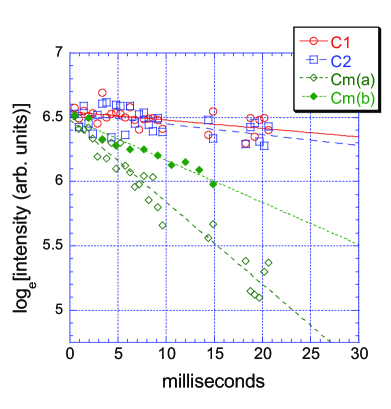
Figure 8: Decay of signal intensity under the dipolar+Hahn refocusing sequence for natural abundance spins in the $1.6\%$ isotopic dilution crystal. $C_{m}(a)$ and $C_{m}(b)$ had TPPM proton decoupling RF power levels of $270$ kHz and $330$ kHz, respectively. Exponential fits to the data indicate effective coherence times (in milliseconds) of [$150$ ($C_{1}$), $120$ ($C_{2}$), $16$ ($C_{m}(a)$), $30$ ($C_{m}(b)$)], although clearly the values obtained for the slower $C_{1}$ and $C_{2}$ decays are more approximate than those for $C_{m}$. Dephasing times $>21$ ms were not explored here due to the heating effects of high-power proton decoupling on the room temperature probe/sample.

V.2 Coherence times under dipolar+Hahn refocusing

Application of a Zeeman and homonuclear dipolar refocusing sequence was investigated, to compare with the simulations of the previous section, and to explore the attainability of longer ¹³C coherence times. The employed sequence is the MREV-8 Haeberlen (1976) dipolar decoupling sequence in combination with a Hahn echo. The pulse spacing of the MREV-8 sequence was set such that one eight-pulse cycle was $240\mu$s in duration. A single $\pi$-pulse was applied in the center of a given dephasing period to refocus the effective Zeeman field Haeberlen (1976) of the MREV-8 sequence (the effective field is in the $\hat{z}-\hat{x}$ plane, so that a $\pi$-pulse about the $\hat{y}$-axis will refocus it). It is a quasi-evolution-suspension sequence because it refocuses like-spin dipolar evolution on a relatively short time-scale compared to the refocusing of Zeeman evolution. Therefore it does not fully remove effective dipolar couplings resulting from unlike-spin $C_{\alpha}$-$C_{\beta}$ couplings (their magnitude will be substantially scaled, however). The data are shown in Figure 8. The decay of the magnetization of the natural abundance spins is shown, since the aim here is to see the effect of refocusing the intermolecular dipolar couplings on coherence times. Monitoring the natural abundance spins is ideal in this regard, since the average intermolecular dipolar environment is identical for all ¹³C spins in the sample, and for the natural abundance spins, it is the only ¹³C dipolar environment. On the other hand, efficient refocusing of the intramolecular couplings would require a shorter MREV-8 sequence, and therefore more pulses for a given dephasing time, yielding greater loss of signal due to pulse imperfections. The ability to suspend the evolution of the qubit spins (e.g. to generate an effective propagator equal to the identity) is an important benchmark for control Ladd et al. (2005) and will be explored in future work.
The coherence times of $C_{1}$ and $C_{2}$ indicated in Fig. 8 (and the corresponding Lorentzian linewidths shown in Table 2) demonstrate a $\sim 50$-fold increase in coherence time compared with the free-induction dephasing times (Table 1). Further, the residual broadening is comparable to the strength of the $C_{\alpha}$-$C_{\beta}$ dipolar interactions, as expected. The coherence time of the methylene carbon $C_{m}$ is clearly limited by the efficiency of proton decoupling. We note that dephasing times $>21$ ms were not explored due to the heating effects of high-power proton decoupling on the room temperature probe/sample. Comparing the Hahn echo and dipolar/Hahn echo data, it is seen that Zeeman shift dispersion contributes $\sim 90$ Hz ($1.2$ ppm) to the free-induction linewidths, whereas the intermolecular dipolar fields contribute $\sim 25$ Hz in the $1.6\%$ dilution crystal. Sequences that efficiently average all spin interactions, such as the Cory 48-pulse sequence Cory et al. (1990), could be used to test the limits of line-narrowing.

VI Discussion

In this paper, we have established benchmark results and described a methodology for controlling solid-state NMR qubits upon which future work can build and improve. High-fidelity quantum control was demonstrated through the preparation of a pseudopure state. That result, along with unitary simulations of the fidelity for the 3-qubit controlled-(not$\otimes$not) gate, suggests that ensemble inhomogeneities involving linear Hamiltonian terms (Zeeman dispersion, RF amplitude) may be suppressed by strongly modulating RF pulses. Additionally, the method of strongly modulating pulses is well-suited to finding solutions for generating arbitrary quantum gates, approaching time-optimality, in systems with complex internal Hamiltonians. Measurement of the triple-quantum dipolar dephasing rate was carried out, as an application of the pseudopure state protocol. Simulations of the intermolecular dipolar field spectrum predicted dipolar linewidths in reasonable agreement with experimental results obtained under appropriate refocusing sequences. Refocusing of the Zeeman and like-spin dipolar terms lead to a $50$-fold increase in ensemble coherence times, and suggests that much narrower effective linewidths could be achieved using sequences that efficiently remove all spin interactions.
These results demonstrate the potential for achieving universal quantum control in solid-state NMR systems with the high precision required for quantum computation and other information processing tasks. Coupled with state purification techniques like dynamic nuclear polarization, such control should enable a powerful new QIP testbed reaching up to $\sim 20-30$ qubits Cory et al. (2000). Furthermore, the solid-state setting is more general than the liquid-state, for example, by allowing one to couple the qubits to a bulk-spin heat bath Cory et al. (2000), as demonstrated by the selective polarization transfer that was employed to begin the pseudopure state protocol. Similar techniques will enable implementation of quantum error correction and heat-bath algorithmic cooling Schulman and Vazirani (1990) protocols, the latter having been already demonstrated in the malonic acid system Baugh et al. (2005).
To further improve control, the strongly modulating pulse optimization procedure must be improved to yield simulated fidelities comparable to those achievable in the liquid state (that is, unitary fidelities in the range of $99-99.9\%$ as opposed to $\sim 95-99\%$). Moreover, the experimental system must be carefully engineered so that the implemented control fields are sufficiently faithful to the simulated pulses. Extending to larger numbers of qubits ($\gtrsim\!12$) will likely require some form of hybrid control that utilizes multiple-pulse, average Hamiltonian techniques in combination with the numerical optimization methods discussed. Additionally, scalable control methods that have been successfully demonstrated in the weak-coupling regime Knill et al. (2000); Negrevergne et al. (2005) could potentially be merged with the strongly modulating pulse methodology to achieve a scalable pulsefinder for appropriately tailored systems that include strongly-coupled spins.
In conclusion, we have characterized in detail a novel solid-state NMR system for quantum information processing, and used it to demonstrate high-fidelity quantum control. This lays a foundation for future studies in the malonic acid system, and in larger systems, desirably with high polarization.