Error Analysis For Encoding A Qubit In An Oscillator

Abstract

In the paper titled “Encoding A Qubit In An Oscillator” Gottesman, Kitaev, and Preskill [quant-ph/0008040] described a method to encode a qubit in the continuous Hilbert space of an oscillator’s position and momentum variables. This encoding provides a natural error correction scheme that can correct errors due to small shifts of the position or momentum wave functions (i.e., use of the displacement operator). We present bounds on the size of correctable shift errors when both qubit and ancilla states may contain errors. We then use these bounds to constrain the quality of input qubit and ancilla states.

Most quantum computation schemes propose encoding qubits using natural two level systems such as spin $1/2$ particles. Others exploit only two states of a larger discrete Hilbert space such as the energy excitation levels of an ion. In the paper “Encoding A Qubit In An Oscillator” Gottesman01 , Gottesman, Kitaev, and Preskill (GKP) described an alternative method for encoding a qubit in the continuous position and momentum degrees of freedom of an oscillator. Because the qubit is encoded in an infinite dimensional Hilbert space, a natural error correcting scheme arises. It can correct errors due to shifts in the oscillator’s position or momentum (i.e., small application of the displacement operator). When the oscillator is chosen to be a single mode of the electromagnetic field, fault tolerant computation can be performed by use of only phase shifters, beam splitters, squeezing, photon counting, and homodyne measurements. Gottesman01 ; Bartlett02 . However, state preparation requires nonlinear interactions.

The GKP scheme constitutes a type of linear optical quantum computer. Other schemes for such computers are based on the proposals of Knill, Laflamme, and Milburn (KLM) Knill00a ; Knill00b ; Knill01 and of Ralph et al. Ralph03 . Of these, the KLM proposal has received most of the analysis Knill00b ; Glancy02 ; Silva04 ; Silva05 ; Dawson05 . However, which (if any) of these three schemes is most suitable for large scale quantum computation is still unknown. Thus, further analysis of all three schemes is required. This paper is devoted to an analysis of the GKP quantum computer. We consider errors only in the input qubit and ancilla states, and we obtain a threshold for the maximum size of position and momentum shifts that the error correcting scheme can always correct. We then use this threshold to constrain the quality of the input states and estimate the number of photons the input states must contain.

We first give a brief review of qubits in the GKP scheme. One may use any type of oscillator to represent a qubit, but for the purposes of this paper we choose the oscillators to be single modes of the electromagnetic field. Let $\hat{a}_{i}$ be the photon annihilation operator of mode $i$, $\hat{a}_{i}^{\dagger}$ the creation operator, $\hat{x}_{i}=1/\sqrt{2}(\hat{a}_{i}^{\dagger}+\hat{a}_{i})$ the $x$-quadrature, and $\hat{p}_{i}=i/\sqrt{2}(\hat{a}_{i}^{\dagger}-\hat{a}_{i})$ the $p$-quadrature. Let $|x\rangle$ denote eigenstates of $\hat{x}$, and $|p\rangle$ eigenstates of $\hat{p}$. We represent the logical 0 qubit as

$$|0_{\text{L}}\rangle = \sum_{s=-\infty}^{\infty}\delta(x-2s\sqrt{\pi})|x\rangle$$ (1)

$$= \frac{1}{\sqrt{2}}\sum_{s=-\infty}^{\infty}\delta(p-s\sqrt{\pi})|p\rangle,$$ (2)

and the logical 1 qubit is

$$|1_{\text{L}}\rangle = \sum_{s=-\infty}^{\infty}\delta(x-(2s+1)\sqrt{\pi})|x\rangle$$ (3)

$$= \frac{1}{\sqrt{2}}\sum_{s=-\infty}^{\infty}(-1)^{s}\delta(p-s\sqrt{\pi})|p\rangle.$$ (4)

In the $x$-quadrature these states are infinitely long combs of delta functions, with the $|1_{\text{L}}\rangle$ displaced a distance $\sqrt{\pi}$ from the $|0_{\text{L}}\rangle$ state. Such states are clearly unphysical, having an infinite energy expectation value, and they are not normalizable.

This encoding can protect the qubits from errors due to displacements in the $x$- and $p$-quadratures, described by the operators $e^{-iu\hat{p}}$ (shifting the $x$-quadrature a distance of $u$) and $e^{-iv\hat{x}}$ (shifting the $p$-quadrature a distance of $v$). These shift operators form a complete basis, so any error superoperator $\mathcal{E}$ acting on the density operator $\rho$ of a single oscillator may be expanded as Gottesman01

$$\mathcal{E}(\rho)=\int\mathrm{d}u\mathrm{d}v\mathrm{d}u^{\prime}\mathrm{d}v^{\prime}F(u,v,u^{\prime},v^{\prime})e^{-iu\hat{p}}e^{-iv\hat{x}}\rho e^{iu^{\prime}\hat{p}}e^{iv^{\prime}\hat{x}}.$$ (5)

If the distribution $F(u,v,u^{\prime},v^{\prime})$ is sufficiently concentrated near the origin, then this encoding allows us to correct $\mathcal{E}$ and recover $\rho$.

Measurement of the qubits can be accomplished by use of homodyne detection of the $x$-quadrature. Results in which the $x$-quadrature is measured to be closer to an even multiple of $\sqrt{\pi}$ are registered as the detection of $|0_{\text{L}}\rangle$, and measurements closer to an odd multiple are registered as $|1_{\text{L}}\rangle$. Therefore, a shift error that is larger than $\sqrt{\pi}/2$ may cause an error in the qubit measurement.

Because the qubit states are unphysical, we must find some states that can approximate the ideal qubit states and are physically realizable. GKP propose using states whose $x$-quadrature wave function is composed of a series of Gaussian peaks of width $\Delta$ contained in a larger Gaussian envelope of width $1/k$. The approximations of the 0 and 1 logical states are

$$\langle x|\tilde{0}\rangle=N_{0}\sum_{s=-\infty}^{\infty}e^{-\frac{1}{2}(2sk\sqrt{\pi})^{2}}e^{-\frac{1}{2}\left(\frac{x-2s\sqrt{\pi}}{\Delta}\right)^{2}}$$ (6)

and

$$\langle x|\tilde{1}\rangle=N_{1}\sum_{s=-\infty}^{\infty}e^{-\frac{1}{2}((2s+1)k\sqrt{\pi})^{2}}e^{-\frac{1}{2}\left(\frac{x-(2s+1)\sqrt{\pi}}{\Delta}\right)^{2}},$$ (7)

where $N_{0}$ and $N_{1}$ are normalization factors. In the limit that $k$ and $\Delta$ are both small, $N_{0}\approx N_{1}=\sqrt{2k}$. We show examples of these approximate qubit states in Fig. 1. First, note that these states are not orthogonal, and there will be some probability of mistaking a 0 state for a 1 state (and a 1 for a 0). This probability is equal to the probability that the $x$-quadrature of the 0 state is measured to be closer to an odd multiple of $\sqrt{\pi}$.

$$P_{0\rightarrow 1}=\sum_{n=-\infty}^{\infty}\int_{2\sqrt{\pi}n+\sqrt{\pi}/2}^{2\sqrt{\pi}(n+1)-\sqrt{\pi}/2}\text{d}x|\langle x|\tilde{0}\rangle|^{2}.$$ (8)

In the limit of small $\Delta$ and $k$, this expression can be approximated as

$$P_{0\rightarrow 1} \approx \frac{2}{\sqrt{\pi}}\sum_{n=0}^{\infty}\int_{\frac{2\sqrt{\pi}n+\sqrt{\pi}/2}{\Delta}}^{\frac{2\sqrt{\pi}(n+1)+\sqrt{\pi}/2}{\Delta}}e^{-y^{2}}\text{d}y$$ (9)

$$\approx \frac{2}{\sqrt{\pi}}\int_{\frac{\sqrt{\pi}}{2\Delta}}^{\infty}e^{-y^{2}}\text{d}y.$$ (10)

For $\Delta=k=0.5$, $P_{0\rightarrow 1}\sim 0.01$, and for $\Delta=k=0.25$, $P_{0\rightarrow 1}\sim 10^{-6}$. For small $\Delta$ and $k$, $P_{1\rightarrow 0}\approx P_{0\rightarrow 1}$. However, we desire not only that measurements can distinguish between the 0 and 1 states, but also that an error correcting procedure can reliably correct errors. This will place stricter requirements on the approximate qubit states.

(a)

(b)

Figure 1: Example approximate qubit states. (a) shows the $x$-quadrature wave function of $|\tilde{0}\rangle$, and (b) shows $|\tilde{1}\rangle$. For each of these we have chosen $\Delta=k=1/4$

We now examine the error correcting circuits. We imagine that the qubit $|Q_{L}\rangle$ initially exists in a superposition of the $|0_{\text{L}}\rangle$ and $|1_{\text{L}}\rangle$ states in mode 1. The qubit then receives errors resulting in shifts of $u_{1}$ in $x_{1}$ and $v_{1}$ in $p_{1}$. We begin the correction procedure by repairing the shifts in $x_{1}$. This requires an ancilla qubit prepared in the state $|+_{\text{L}}\rangle=|0_{\text{L}}\rangle+|1_{\text{L}}\rangle$ in mode 2. Of course, the ancilla may also be subject to errors, resulting in shifts $u_{2}$ and $v_{2}$. After the errors, the state of the system is

$$e^{-iu_{1}\hat{p}_{1}}e^{-iv_{1}\hat{x}_{1}}e^{-iu_{2}\hat{p}_{2}}e^{-iv_{2}\hat{x}_{2}}|Q_{\text{L}}\rangle_{1}|+_{\text{L}}\rangle_{2}.$$ (11)

To correct the qubit’s errors, modes 1 and 2 are sent through the network pictured in Fig. 2. The two damaged modes meet in a beam splitter, which performs the transformation

$$x_{1} \rightarrow \frac{1}{\sqrt{2}}\left(x_{1}-x_{2}\right)$$ (12)

$$x_{2} \rightarrow \frac{1}{\sqrt{2}}\left(x_{1}+x_{2}\right)$$ (13)

in the $x$-quadrature wave function of the two modes. After mode 1 exits the beam splitter, we apply the squeezing operator $\hat{S}(\sqrt{2})$, where $\hat{S}$ is defined by $\hat{S}(q)|x\rangle=\sqrt{q}|x/q\rangle$. We now measure the $x$-quadrature of mode 2 and obtain the result $x_{2}=1/\sqrt{2}\left(n\sqrt{\pi}-u_{1}-u_{2}\right),$ where $n$ may be any integer. This measurement provides some information about the errors shifting the $x$-quadrature of the qubit. The errors can be (partially) corrected by applying the displacement operator $e^{-is(x_{2})\hat{p}_{1}}$, where

$$s(q)=-\frac{q}{\sqrt{2}}+\frac{1}{2}\text{Mod}_{2\sqrt{\pi}}\left(2\sqrt{2}q\right).$$ (14)

Here the Mod function has the range $[-\sqrt{\pi},\sqrt{\pi})$.

Figure 2: Procedure to correct $x$ shifts acting on the qubit. The circuit shows errors acting on the qubit and ancilla. Then the qubit and ancilla modes meet in a beam splitter, mode 1 is squeezed, the $x$-quadrature of mode 2 is measured, and a correcting shift of $s(x_{2})$ is applied to the qubit.

This entire sequence of operations – errors and correction procedure – transforms the qubit to the state

$$|Q_{\text{L}}\rangle \rightarrow e^{i\phi(u_{1},v_{1},u_{2},v_{2},n)}e^{-i(v_{1}-v_{2})\hat{x}_{1}}$$ (15)

$$\times e^{-i\left(u_{1}-\frac{1}{2}\text{Mod}_{2\sqrt{\pi}}\left(2u_{1}+2u_{2}\right)\right)\hat{p}_{1}}|Q_{\text{L}}\rangle,$$

where $e^{i\phi(u_{1},v_{1},u_{2},v_{2},n)}$ is a phase factor independent of the input qubit. If $|u_{1}+u_{2}|<\sqrt{\pi}/2$, then the qubit is “corrected” to the state

$$|Q_{\text{L}}\rangle \rightarrow e^{i\phi(u_{1},v_{1},u_{2},v_{2},n)}e^{-i(v_{1}-v_{2})\hat{x}_{1}}$$ (16)

$$\times e^{-iu_{2}\hat{p}_{1}}|Q_{\text{L}}\rangle.$$

Notice that both the ancilla and the qubit’s $p$ shift errors $v_{1}$ and $v_{2}$ both appear now acting on the qubit. Also, the qubit has been affected by the ancilla’s $x$ shift error $u_{2}$. In the case when $|u_{1}+u_{2}|>\sqrt{\pi}/2$, the error correcting procedure applies the Pauli $X$ operator to the qubit state, producing

$$|Q_{\text{L}}\rangle \rightarrow e^{i\phi(u_{1},v_{1},u_{2},v_{2},n)}e^{-i(v_{1}-v_{2})\hat{x}_{1}}$$ (17)

$$\times e^{-iu_{2}\hat{p}_{1}}X|Q_{\text{L}}\rangle.$$

Correcting the $X$ error would require the use of a standard quantum error correcting code (concatenated with this continuous variable code). See Nielsen00 for an introduction to quantum error-correcting codes.

Figure 3: Procedure to correct $p$ shifts acting on the qubit. The circuit shows errors acting on the qubit and ancilla. Then the qubit and ancilla modes meet in a beam splitter, mode 1 is squeezed, the $p$-quadrature of mode 2 is measured, and a correcting shift of $s(p_{2})$ is applied to the qubit.

The procedure for correcting shifts to the qubit’s $p$-quadrature wave function is similar to that used for $x$ shifts. It is pictured in Fig. 3. In this case we prepare the ancilla qubit in the state $|0_{\text{L}}\rangle$, we measure the $p$-quadrature basis of mode 2, we apply the squeezing operator $\hat{S}(1/\sqrt{2})$, and the correcting shift is $e^{-is(p_{2})\hat{x}_{1}}$. The errors and correcting procedure produces the new state

$$|Q_{\text{L}}\rangle \rightarrow e^{i\theta(u_{1},v_{1},u_{2},v_{2},n)}e^{-i(u_{1}-u_{2})\hat{p}_{1}}$$ (18)

$$\times e^{-i\left(v_{1}-\frac{1}{2}\text{Mod}_{2\sqrt{\pi}}\left(2v_{1}+2v_{2}\right)\right)\hat{x}_{1}}|Q_{\text{L}}\rangle,$$

where the phase factor $e^{i\theta(u_{1},v_{1},u_{2},v_{2},n)}$ is independent of the initial qubit state. When $|v_{1}+v_{2}|<\sqrt{\pi}/2$ the correcting procedure is successful, resulting in the state

$$|Q_{\text{L}}\rangle \rightarrow e^{i\theta(u_{1},v_{1},u_{2},v_{2},n)}e^{-i(u_{1}-u_{2})\hat{p}_{1}}$$ (19)

$$\times e^{-iv_{2}\hat{x}_{1}}|Q_{\text{L}}\rangle.$$

When $v_{1}$ and $v_{2}$ are too large, the correcting circuit creates a Pauli $Z$ error in the logical qubit basis.

Armed with a clear understanding of the error correction procedure, we can formulate a bound on the maximum error that this scheme can always correct. In the following we imagine that the only error source is in the preparation of the qubit and ancilla states. We assume that all of the operations of the error correcting procedure are error free. In the above analysis we have shown how errors in ancillas are transferred to the qubit. We would like to find a bound on the size of shift errors affecting the qubit and ancillas that ensures that the qubit never receives an $X$ or $Z$ error and that the sizes of $x$ and $p$ shifts do not grow after multiple steps of error correction. To accomplish this we follow the qubit’s $x$ and $p$ shifts as it passes through multiple steps of correction.

Before the error correction procedure, the qubit has errors $u_{1}$ and $v_{1}$, and the first ancilla has errors $u_{2}$ and $v_{2}$. If we first correct errors of the $x$-quadrature, the qubit will have errors $u_{2}$ (in $x$) and $v_{1}-v_{2}$ (in $p$), provided that $|u_{1}+u_{2}|<\sqrt{\pi}/2$. This result comes directly from Eq. (16). Now, we should correct errors of the $p$-quadrature using a new ancilla, which may have errors $u_{3}$ and $v_{3}$. The $p$ error correction produces a new qubit with errors $u_{2}-u_{3}$ (in $x$) and $v_{3}$ (in $p$), provided that $|v_{1}-v_{2}+v_{3}|<\sqrt{\pi}/2$. At this point, the first stage of error correction is complete. The qubit’s original errors have been entirely eliminated and replaced by errors introduced by the ancillas. A second correction of the $x$-quadrature using a third ancilla with errors $u_{4}$ and $v_{4}$ is successful if $|u_{2}-u_{3}+u_{4}|<\sqrt{\pi}/2$. The qubit now has errors $u_{4}$ and $v_{3}-v_{4}$. In this and each subsequent stage, we find that at any time, the qubit has errors inherited from one ancilla in the quadrature that was just corrected and errors from two ancillas in the quadrature, which should be corrected next. During the next correction errors from a new ancilla are introduced. The correction succeeds if the magnitudes of the now three errors is less than $\sqrt{\pi}/2$. Therefore, we can be certain that repeated error correction steps will be successful if the magnitude of all errors shifts are smaller than $\sqrt{\pi}/6$.

We would now like to calculate the probability that an approximate qubit state such as $|\tilde{0}\rangle$ or $|\tilde{1}\rangle$ has shifts smaller than $\sqrt{\pi}/6$ in both $x$- and $p$-quadratures. To find this probability we decompose the approximate qubit states in a basis defined by the states that are $x$- and $p$-shifts of $|0_{\text{L}}\rangle$, which we may express as

$$|u,v\rangle = \pi^{-1/4}e^{-iu\hat{p}}e^{-iv\hat{x}}|0_{\text{L}}\rangle$$ (20)

$$= \pi^{-1/4}\sum_{s=-\infty}^{\infty}e^{-iv2s\sqrt{\pi}}|x=2s\sqrt{\pi}+u\rangle.$$ (21)

We can express any state $|\psi\rangle$ of a single oscillator in this basis using a wave function $f(u,v)=\langle u,v|\psi\rangle$:

$$|\psi\rangle=\int_{-\sqrt{\pi}}^{\sqrt{\pi}}\text{d}u\int_{-\frac{\sqrt{\pi}}{2}}^{\frac{\sqrt{\pi}}{2}}\text{d}vf(u,v)|u,v\rangle.$$ (22)

The limits of the above integral are chosen to match the periodicity in $|0_{\text{L}}\rangle$. The probability density for a state having shifts $u$ and $v$ from $|0_{\text{L}}\rangle$ is simply

$$P(u,v)=|f(u,v)|^{2}.$$ (23)

Examples of $P(u,v)$ are shown in figures 4 and 5.

Figure 4: $P(u,v)$ the probability density that the $|\tilde{0}\rangle$ approximate qubit state contains errors $u$ (in its $x$-quadrature) and $v$ (in its $p$-quadrature). Here we have used $\Delta=k=1/4$.

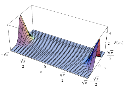
Figure 5: $P(u,v)$ the probability density that the $|\tilde{1}\rangle$ approximate qubit state contains errors $u$ (in its $x$-quadrature) and $v$ (in its $p$-quadrature). Here we have used $\Delta=k=1/4$.

The probability that the $|\tilde{0}\rangle$ state has errors less than $\sqrt{\pi}/6$ (which guarantees that its errors may always be corrected) is

$$P_{\text{no error}}=\int_{-\frac{\sqrt{\pi}}{6}}^{\frac{\sqrt{\pi}}{6}}\text{d}u\int_{-\frac{\sqrt{\pi}}{6}}^{\frac{\sqrt{\pi}}{6}}\text{d}vP(u,v).$$ (24)

We plot $P_{\text{no error}}$ in Fig. 6. Achieving $P_{\text{no error}}=0.9$ requires $\Delta=k=0.214$, and $P_{\text{no error}}=0.99$ requires $\Delta=k=0.149$.

Figure 6: Here we plot $P_{\text{no error}}$, the probability that an approximate qubit state has shifts in both $x$- and $p$-quadratures less than $\sqrt{\pi}/6$ as a function of $\Delta=k$. This shows the case of $|\tilde{0}\rangle$, but the $|\tilde{1}\rangle$ plot is indistinguishable.

We generally believe that protecting an oscillator from decoherence usually becomes more difficult when the oscillator contains large numbers of photons, so we are motivated to calculate the mean number of photons in the approximate qubit states. A crude estimate of this quantity for small $\Delta$ and $k$ is given by

$$\langle n\rangle\sim\frac{1}{4\Delta^{2}}+\frac{1}{4k^{2}}.$$ (25)

In Fig. 7 we plot the mean number of photons contained in an approximate qubit state as a function of $P_{\text{error}}=1-P_{\text{no error}}$ using an exact expression. We find that an approximate qubit state with $P_{\text{no error}}=0.9$ must contain $\langle n\rangle=10.4$ photons, and to achieve $P_{\text{no error}}=0.99$ requires $\langle n\rangle=22.1$ photons.

Figure 7: Here we plot the mean number of photons contained in an approximate qubit state as a function of the probability that such a state has a shift error larger than $\sqrt{\pi}/6$.

Production of these states is likely to be very challenging. We are aware of four proposals for production of qubit states for the GKP quantum computer. The first is from the original work of GKP Gottesman01 , in which they propose the use of a two-mode Hamiltonian of the form $\hat{x}_{1}\hat{n}_{2}$. This might be achieved by coupling an optical mode with a mirror that may exist in a coherent superposition of position states. For a discussion of the possibility of such experiments see Giovannetti00 ; Pinard05 and their references. The second proposal is from Travaglione and Milburn Travaglione02 . They describe a method that prepares the qubit states in the oscillatory motion of a trapped ion rather than the photons in an optical mode. The third proposal is by Pirandola et al. Pirandola04 and discusses the preparation of optical GKP states using a two mode Kerr interaction (described by a Hamiltonian of the form $\hat{n}_{1}\hat{n}_{2}$) followed by a homodyne measurement of one of the modes. The same authors also describe a fourth method for GKP state production in Pirandola05a ; Pirandola05b . This method would prepare the GKP state in the motion of a neutral atom that interacts with a photon field confined to a high finesse optical cavity. They show that this may be done so that the atom is trapped in the cavity, or the atom may be free to pass through the cavity. State preparation is currently the most problematic aspect of the GKP quantum computation scheme, and it is an area in need of more experimental effort.

In this paper we have investigated error correction in the GKP quantum computer, considering errors in both qubit and ancilla states. Provided that all input states have displacement errors in their $x$- and $p$-quadratures less than $\sqrt{\pi}/6$, the error correction schemes will operate successfully. Because it is impossible to prepare perfectly error free GKP states, we have calculated the probability that approximate GKP states contain an error larger than $\sqrt{\pi}/6$. An approximate GKP state with error probability less than $0.1$ must contain a mean number of photons greater than $10.4$.

There are some cases in which states with errors larger than $\sqrt{\pi}/6$ will not cause logical qubit errors. For example, the qubit’s and the ancilla’s errors may actually cancel one another. Because of effects like this, our $\sqrt{\pi}/6$ bound may be refined with more detailed analysis. We have not considered full fault tolerant computation in the presence of noisy logic operations, nor have we considered the effects of phase errors or photon absorption. Phase errors and photon absorption are likely to be primary error sources for this (or any) optical quantum computer. Because linear superpositions of displacements span the space of possible single qubit errors, one may correct phase and absorption errors using the GKP error correction scheme. However, phase errors affecting states with large numbers of photons correspond to large displacements. This fact highlights two competing influences: (1) To lower the number of intrinsic errors in each approximate qubit state, we must prepare states with large numbers of photons. (2) To reduce the displacements caused by phase errors, we should prepare states with fewer photons. A detailed analysis of these constraints requires further study.

Acknowledgments We thank Hilma Vasconcelos and Rich Mirin for helpful comments on the manuscript.

References

- (1) Daniel Gottesman, Alexi Kitaev, and John Preskill “Encoding A Qubit In An Oscillator” Physical Review A 64, 012310 (2001), e-print quant-ph/0008040.
- (2) Stephen D. Bartlett and Barry C. Sanders, “Universal Continuous-Variable Quantum Computation: Requirement Of Optical Nonlinearity For Photon Counting” Physical Review A 65, 042304 (2001), e-print quant-ph/0110039.
- (3) E. Knill, R. Laflamme, and G. Milburn, “Efficient Linear Optics Quantum Computation” (2000), e-print quant-ph/0006088.
- (4) E. Knill, R. Laflamme, and G. Milburn, “Thresholds For Linear Optics Quantum Computation” (2000), e-print quant-ph/0006120.
- (5) E. Knill, R. Laflamme, and G. Milburn, “A Scheme For Efficient Quantum Computation With Linear Optics” Nature 409, 46 (2001).
- (6) T. C. Ralph, A. Gilchrist, G. J. Milburn, W. J. Munro, and S. Glancy, “Quantum Computation With Optical Coherent States.” Physical Review A 68, 042319 (2003), e-print quant-ph/0306004.
- (7) S. Glancy, J. M. LoSecco, H. M. Vasconcelos, and C. E. Tanner, “Imperfect Detectors In Linear Optical Quantum Computers” Physical Review A 65, 062317 (2002), e-print quant-ph/0201047.
- (8) Marcus Silva, “Erasure Thresholds For Efficient Linear Optics Quantum Computation” (2004), e-print quant-ph/0405112.
- (9) Marcus Silva, Martin Roettler, and Christof Zalka, “Thresholds For Linear Optics Quantum Computing With Photon Loss At The Detectors” Physical Review A 72, 032307 (2005), e-print quant-ph/0502101.
- (10) Christopher M. Dawson, Henry L. Haselgrove, and Michael A. Nielsen, “Noise Thresholds For Optical Quantum Computers” (2005), quant-ph/0509060.
- (11) Michael A. Nielsen and Isaac L. Chuang, Quantum Computation And Quantum Information (Cambridge University Press, Cambridge, 2000).
- (12) Vittorio Giovannetti, Stefano Mancini, and Paolo Tombesi, “Radiation Pressure Induced Einstein-Podolsky-Rosen Paradox” Europhysics Letters 54, 559 (2001), e-print quant-ph/0005066.
- (13) Michel Pinard, Aurelien Dantan, David Vitali, Olivier Arcizet, Tristan Briant, Antoine Heidmann, “Entangling Movable Mirrors In A Double Cavity System” (2005), e-print quant-ph/0507275.
- (14) B. C. Travaglione and G. J. Milburn, “Preparing Encoded States In An Oscillator” Physical Review A 66, 052322 (2002), e-print quant-ph/0205114.
- (15) S. Pirandola, S. Mancini, D. Vitali, and P. Tombesi, “Constructing Finite Dimensional Codes With Optical Continuous Variables” Europhysics Letters 68, 323 (2004), e-print quant-ph/0402202.
- (16) Stefano Pirandola, Stefano Mancini, David Vitali, and Paolo Tombesi, “Continuous Variable Encoding By Pondermotive Interaction” (2005), e-print quant-ph/0503003.
- (17) Stefano Pirandola, Stefano Mancini, David Vitali, and Paolo Tombesi, “Generating Continuous Variable Quantum Codewords In The Near-Field Atomic Lithography” (2005), e-print quant-ph/0510053.