Manipulating quantum information by propagation

Abstract

We study creation of bi- and multipartite continuous variable entanglement in structures of coupled quantum harmonic oscillators. By adjusting the interaction strengths between nearest neighbors we show how to maximize the entanglement production between the arms in a Y-shaped structure where an initial single mode squeezed state is created in the first oscillator of the input arm. We also consider the action of the same structure as an approximate quantum cloner. For a specific time in the system dynamics the last oscillators in the output arms can be considered as imperfect copies of the initial state. By increasing the number of arms in the structure, multipartite entanglement is obtained, as well as $1\rightarrow M$ cloning. Finally, we are considering configurations that implement the symmetric splitting of an initial entangled state. All calculations are carried out within the framework of the rotating wave approximation in quantum optics, and our predictions could be tested with current available experimental techniques.

I Introduction

Generally quantum information processing is considered theoretically and implemented experimentally as a temporal sequence of quantum gates applied to quantum bits that are stationary in space. Many classical information processing devices function differently however. A microchip usually takes as an input currents that are propagating through the chip where they suffer classical logic gates. The emerging current represent the outcome of the particular classical operation that has been carried out. In the present work we consider the quantum information equivalent of this way of processing information, ie we propagate quantum information through a system of interacting quantum systems such that, in the course of its propagation through the system, it suffers a non-trivial quantum state transformation. In the following we will focus attention on harmonic chains for their ready availability of exact solutions in non-trivial settings with many excitations Eisert P 03 ; Eisert PBH 03 ; Plenio HE 04 ; Plenio S 05 ; McAneney PK 05 ; Paternostro KPL 05 but see also recent work in spin-systems in this direction Yung B 05 ; Hadley SB 05

The aim is to design devices to be integrated in a quantum information processor in which it will be essential the availability of reliable sources of entanglement as well as its transportation and unitary manipulation inside the processor. At the same time the proposed structures can be considered as cloning machines of one initial input state.

This paper is structured as follows. In Section II we present the basic physical model and its Hamiltonian as well as the utilized tools to measure entanglement and its time evolution in the system. In section III we describe the Y-shaped structure formed by coupled quantum harmonic oscillators, and fix the initial conditions for entanglement creation. We present and justify the required tuning of the coupling strengths between nearest neigbours that creates maximum entanglement between the last oscillators in the output arms, and provide the resulting unitary transformation between initial and final states. We show different results varying the system parameters and compare them with previous ones and with the upper limit for entanglement generation in the system. Then we extend the result to multiarm structures in which multipartite entanglement is created. Finally we study X-shaped structures which work as entanglement beam splitters. In Section IV we study the action of the same structures as a cloning machines in which the final states in the last oscillators of the output arms can be considered as imperfect copies of the initial input state. We provide the fidelity expression in terms of the squeezing parameter and also extend the results to multiarm structures which creates multiple more imperfect copies.

II Model and analytical tools

We begin by introducing the basic technical tools that we will be employing in this work.

II.1 Hamiltonian

We begin by briefly describing the model system used in Ref. Plenio HE 04 , a 1D chain of interacting quantum harmonic oscillators, and the tools used to describe quantum states and entanglement in it. In the rotating wave approximation (RWA) the Hamiltonian of the system is given by

$$\hat{H}=\sum_{k=1}^{M}\left[(1+c)\Bigl{(}{\hat{a}}^{\dagger}_{k}{\hat{a}}_{k}+\frac{1}{2}\Bigr{)}-c\left(\hat{a}^{\dagger}_{k+1}\hat{a}_{k}+\hat{a}_{k+1}\hat{a}^{\dagger}_{k}\right)\right].$$ (1)

We may rewrite this Hamiltonian in terms of position and momentum operators ${\hat{q}}_{k}$ and ${\hat{p}}_{k}$ as is customary in a large part of the quantum information literature. Defining ${\hat{a}}=({\hat{q}}+i{\hat{p}})/\sqrt{2}$ and ${\hat{a}}^{\dagger}=({\hat{q}}-i{\hat{p}})/\sqrt{2}$ we find

$$\hat{H}=\frac{1}{2}\sum_{k=1}^{M}\left[{\hat{q}}_{k}^{2}+{\hat{p}}_{k}^{2}+\frac{c}{2}\left(\hat{q}_{k+1}-\hat{q}_{k}\right)^{2}+\frac{c}{2}\left(\hat{p}_{k+1}-\hat{p}_{k}\right)^{2}\right],$$ (2)

where $c$ is the coupling constant between next neighbors. In this paper we will use its matrix form

$$\hat{H}=\frac{1}{2}R\left[\begin{array}[]{cc}V&0\\ 0&T\end{array}\right]R^{T}=\frac{1}{2}\sum_{ij=1}^{M}{\hat{q}}_{i}V_{ij}{\hat{q}}_{j}+{\hat{p}}_{i}T_{ij}{\hat{p}}_{j},$$ (3)

where $R^{T}=({\hat{q}}_{1},\ldots,{\hat{q}}_{n},{\hat{p}}_{1},\ldots,{\hat{p}}_{n})$, and $V$, $T$ are the potential and kinetic matrices respectively Audenaert EPW 02 . In the rotating wave approximation we find $V=T$.

II.2 Gaussian states

Analysing the entanglement properties of infinite dimensional systems is generally technically involved unless one restricts attention to so-called Gaussian states Eisert P 03 ; Simon SM 87 , which are more easily described in phase space introducing the (Wigner-)characteristic function. Using the Weyl operator $W_{\xi}=e^{i\xi^{T}R}$ for $\xi\in{\mathbf{R}}^{2n}$ we define the characteristic function as

$$\chi_{\rho}(\xi)=\mbox{tr}[\rho W_{\xi}].$$ (4)

The state and its characteristic function are related to each other according to a Fourier-Weyl relation,

$$\rho=\frac{1}{(2\pi)^{n}}\int d^{2n}\xi\chi_{\rho}(-\xi)W_{\xi}.$$ (5)

Gaussian states are exactly those states for which the characteristic function $\chi_{\rho}$ is a Gaussian function in phase space Simon SM 87 and are completely specified by their first and second moments, $d$ and $\gamma$

$$\chi_{\rho}(\xi)=\chi_{\rho}(0)e^{-\frac{1}{4}\xi^{T}\gamma\xi-d^{T}\xi}.$$ (6)

As the first moments can be always made zero utilizing appropriate local displacements in phase space, they are not relevant in the context of questions related to squeezing and entanglement and will be ignored in the following. The second moments can be collected in the real symmetric $2n\times 2n$ covariance matrix $\gamma$ defined as

$$\gamma_{j,k} = 2\mbox{Re}\,\mbox{tr}\left[\rho\left({\hat{R}}_{j}-\langle{\hat{R}}_{j}\rangle_{\rho}\right)\left({\hat{R}}_{k}-\langle{\hat{R}}_{k}\rangle_{\rho}\right)\right].$$ (7)

With this convention, the covariance matrix of the $n$-mode vacuum is $\gamma={\sf 1\rule[0.04303pt]{0.51663pt}{6.54443pt}\rule[0.04303pt]{1.29167pt}{0.51663pt}}_{2n}$.

For a Hamiltonian operator like (3) we find that the covariance matrix of the ground state is Audenaert EPW 02

$$\gamma=\sqrt{TV^{-1}}\oplus\sqrt{VT^{-1}}$$ (8)

In RWA we have $T=V$ and the ground state is given by $\gamma={\sf 1\rule[0.04303pt]{0.51663pt}{6.54443pt}\rule[0.04303pt]{1.29167pt}{0.51663pt}}_{n}\oplus{\sf 1\rule[0.04303pt]{0.51663pt}{6.54443pt}\rule[0.04303pt]{1.29167pt}{0.51663pt}}_{n}$, which is the same as the ground-state of $n$ non-interacting harmonic oscillators.

II.3 Entanglement of Gaussian States

As the covariance matrix encodes the complete information about the entanglement properties of the a Gaussian state, we will use it in order to quantify the amount of entanglement between two groups of oscillators. In this work we are going to use two entanglement measures. When considering pure states, the appropriate measure of entanglement is the entropy of entanglement which is defined as the von-Neumann entropy of the reduced density matrix of one subsystem. In the Gaussian states setting this reduced density matrix is again described by a covariance matrix $\gamma_{A}$ and the displacements. As displacements represent local unitary basis changes they are irrelevant when considering the entanglement properties of a Gaussian state. If we denote the symplectic eigenvalues of $\gamma_{A}$ describing $m$ harmonic oscillators by $\mu_{i}$ we find Plenio EDC 05 for the entropy of entanglement the expression

$$S=\sum_{i=1}^{m}\left(\frac{\mu_{i}+1}{2}\log_{2}\frac{\mu_{i}+1}{2}-\frac{\mu_{i}-1}{2}\log_{2}\frac{\mu_{i}-1}{2}\right).$$ (9)

Another measure of entanglement that can also be applied for mixed quantum states is the logarithmic negativity Lewenstein HSL 98 ; Eisert P 99 ; Lee KPL 00 ; Eisert Phd ; Vidal W 02 ; Plenio V 05 . This measure is easy to compute, possesses an interpretation as a cost function Audenaert PE 03 and its monotonicity under local operations and classical communication has been proven recently Plenio 05 . Given two parties, $A$ and $B$, that consist of $m$ and $n$ harmonic oscillators respectively, the logarithmic negativity is defined as

$$N(\rho)=\log_{2}||\rho^{T_{B}}||_{1}=-\sum_{j=1}^{m+n}\log_{2}(\min(1,|\gamma_{j}|)),$$ (10)

where $\rho^{T_{B}}$ is the partial transposition of $\rho$ with respect to system $B$, and $||.||_{1}$ denotes the trace-norm. The second equality is obtained employing the symplectic eigenvalues $\gamma_{j}$ of the covariance matrix $\gamma^{T_{B}}$ corresponding to the partially transposed state $\rho^{T_{B}}$ (see Refs. Audenaert EPW 02 ; Plenio HE 04 ).

II.4 The equations of motion

As we are interested in the entanglement evolution we must now find equations of motion for the covariance matrix. The dynamics of the covariance matrix under a Hamiltonian quadratic in position and momentum operators can be obtained straightforwardly from the Heisenberg equation.

$$\frac{d}{dt}\hat{X}(t)=i[{\hat{H}},\hat{X}].$$ (11)

For our time-independent Hamiltonian Eq. (3), this leads to the covariance matrix at time $t$ as

$$\Gamma(t)=\exp^{\left({\left[\begin{array}[]{cc}0&T\\ -V&0\\ \end{array}\right]t}\right)}\Gamma(0)\exp^{\left({\left[\begin{array}[]{cc}0&-V\\ T&0\\ \end{array}\right]t}\right)}.$$ (16)

where

$$\Gamma(t):=\left(\begin{array}[]{cc}\gamma_{XX}&\gamma_{XP}\\ \gamma_{PX}&\gamma_{PP}\\ \end{array}\right)(t).$$ (19)

These equations of motion will be numerically integrated and, in some cases, analytically be solved in this paper.

III Creating entanglement by propagation

We begin our considerations by devising structures in which entanglement is generated automatically during the propagation of quantum information.

III.1 Bipartite entanglement

In Ref. Plenio HE 04 a Y-shaped structure as shown in Fig. 1 was proposed. One arm, the input arm, consisting of $M_{\rm in}$ oscillators is connected to two further arms, the output arms, each consisting of $M_{\rm out}$ oscillators. Only nearest neighbour interactions are considered and it is assumed that the structure is initially in the ground state, i.e., at temperature $T=0$. At time $t=0$ we perturb the first harmonic oscillator in the input arm exciting it either to a thermal state characterized by covariance matrix elements $\gamma_{q_{1}q_{1}}=\gamma_{p_{1}p_{1}}=z$ for some $z$, or a pure squeezed state characterized by covariance matrix elements $\gamma_{q_{1}q_{1}}=1/\gamma_{p_{1}p_{1}}=z$

$$\gamma_{1}(t=0)=\left[\begin{array}[]{cccccc}z&0\\ 0&1/z\end{array}\right].$$ (20)

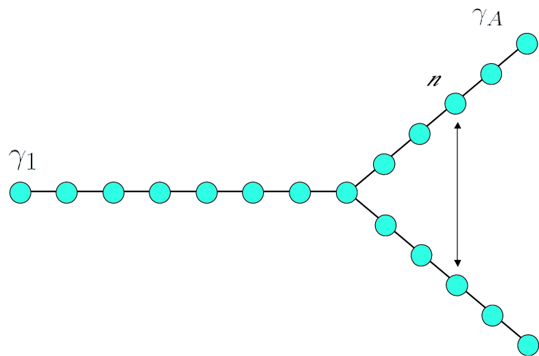
Figure 1: Sketch of the Y-shaped structure. A single input arm consists of $M_{\rm in}$ oscillators (here $8$) is connected to two output arms each consisting of $M_{\rm out}$ oscillators (here $5$). The arrow indicates how to group oscillators in the same position $n$ of each branch to apply basis change (24).

We observe that for an initial thermal state excitation no entanglement is ever found between the ends of the two arms of the Y-shape. This can be understood from the observation that a thermal state is a mixture of coherent states, i.e., displaced vacuum states. Displacements do not contribute to the entanglement in a state so that it is sufficient to consider the vacuum state. If the system is initialized in the vacuum state however it remains stationary and will evidently not lead to any entanglement as long as we are considering the RWA. Therefore an initialization in a thermal state cannot yield entanglement either.

For a squeezed state input on the other hand a considerable amount of entanglement is generated. These two observations are resembling closely optical beamsplitters which do not create entanglement from thermal state input but can generate entanglement from squeezed inputs (see Ref. Wolf EP 03 for a comprehensive treatment of the entangling capacity of linear optical devices).

It is now natural to consider which nearest neighbour coupling provides the optimal generation of entanglement. These optimal couplings can be found numerically by adjusting randomly individual couplings, accepting changes that improve the amount of entanglement that is being generated in the structure at a given time for a given input. The results so obtained provide the intuition by which one then arrives at an analytical argument. In Ref. Plenio HE 04 it was shown that it is possible to obtain perfect transmission in a linear chain of $M$ oscillators if the couplings are adjusted in a square root law

$$V_{n,n+1} = V_{n+1,n}=\frac{c}{2}\sqrt{n(M-n)}$$ (21)

$$V_{n,n} = 1.$$ (22)

With this potential matrix an interchange between the first and the $M$-th coordinate occurs by waiting for a time $t=\pi/c$ (see Ref. Christandl DEL 03 for an analogous argument in spin chains).

To obtain the equivalent perfect transmission distributed between the arms in the Y-shaped structure, we must modify the coupling strengths between the oscillator in the junction and the first two oscillators in the arms, $V_{M_{\rm in},M_{\rm in}+1}$, in the following way

$$V_{M_{\rm in},M_{\rm in}+1}=\frac{c}{2}\sqrt{M_{\rm in}(M-M_{\rm in})/2}.$$ (23)

In Fig. 2 these couplings are shown for $M_{\rm in}=8$ and $M_{\rm out}=5$.

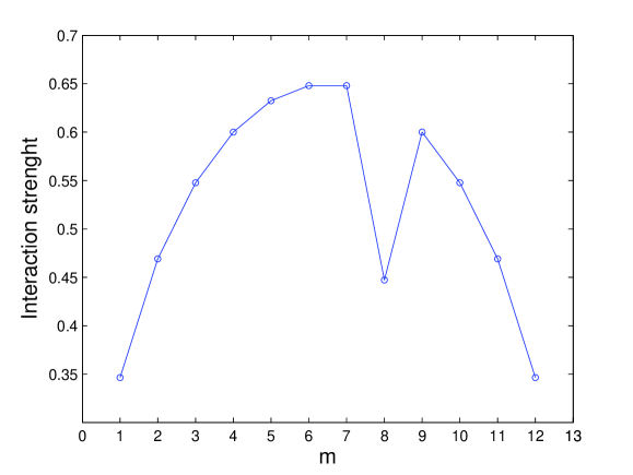
Figure 2: Square root law profile of the potential matrix non-diagonal elements which produces maximum entanglement between both final oscillators in the output arms of the Y-shaped structure (just one output arm interactions are shown). The coupling between the last oscillator in the input arm, and the first oscillator in the output arms must be divided by $\sqrt{2}$. $M_{\rm in}=8$, $M_{\rm out}=5$ and $c=0.2$.

To understand the origin of this choice of coupling strengths we link it to perfect transmission in a linear chain. Indeed, with a basis change between both systems it can be proved that the choice of coupling for the Y-shape corresponds to perfect transmission in a linear structure consisting of the incoming arm and one outgoing arm while the other outgoing arm is becoming decoupled (see Fig. 3). Labelling the two arms with $A,B$ we take oscillators by pairs in the same position $n$ of each arm, and make the following change just in arms (see Fig. 1)

$${\hat{q}}_{n}^{A}=\frac{1}{\sqrt{2}}({\hat{Q}}_{n}^{A}+{\hat{Q}}_{n}^{B}),\;\;\;\;\;{\hat{q}}_{n}^{B}=\frac{1}{\sqrt{2}}({\hat{Q}}_{n}^{A}-{\hat{Q}}_{n}^{B}),$$ (24)

with analogous equations for momentum operators ${\hat{p}}_{n}$. Introducing this change in the expression for the system Hamiltonian (2) we obtain that $A$ arm gets the perfect transmission coupling strengths Eq. (21), while $B$ arm is decoupled.

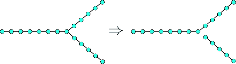
Figure 3: Under the transformation (24) the Y-shape on the left hand side is transformed into a linear chain consisting of the input arm and one output arm while the other output arm is now decoupled.

How does this allow us to obtain the optimal couplings for the y-shape? First, we consider the transformed y-shape depicted on the right hand side of fig. 3. We perform the same procedure carried out for the linear chain (see Ref. Plenio HE 04 for an analytical proof of optimality) to obtain the optimized couplings for this situation. Transforming back to the original coordinates, ie the situation on the left hand side of Fig. 3, we then obtain the coupling strengths suggested in eqs. (21-23). This then implies that the initially squeezed state is, in the transformed picture, transmitted perfectly to the end of the outgoing arms. Inverting the transformation, which is indeed the same transformation as that implemented by a 50/50 beamsplitter, we then obtain a two-mode squeezed state in the original picture. The results in Wolf EP 03 imply that the transformation corresponding to a 50/50 beamsplitter is the optimal linear optics entangling transformation for an initial squeezed state. This implies that the procedure as a whole, ie the choice of couplings, is optimal – at least in the Gaussian setting. If the initial quantum state of the first oscillator is squeezed the final states in the last oscillators in the present maximum entanglement at that time, as can be observed in Fig. 4, where logarithmic negativity is shown. The only effect of increasing the number of oscillators (adjusting couplings accordingly) is to narrow the peaks without decreasing the maximum entanglement. This is contrasted by the behaviour of a system in which all the couplings between nearest neighbours are equal. Then the magnitude of the entanglement decreases as the number of oscillator increases, and irregular time patterns are obtained Plenio HE 04 .

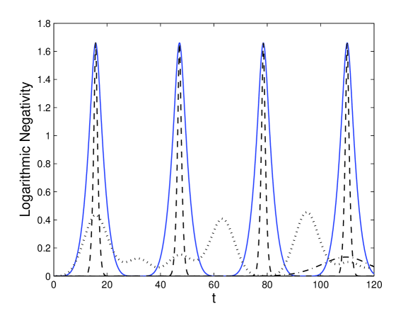
Figure 4: Time evolution of entanglement between the two last oscillators in the Y-shaped structure when an initial squeezed state is prepared in the first oscillator of the input arm. Maximum entanglement is obtained for $t=\pi/c$. Solid line corresponds to $M_{\rm in}=M_{\rm out}=2$ and dashed line to $M_{\rm in}=M_{\rm out}=20$. Dotted and dash-dotted lines correspond to RWA Hamiltonian with constant couplings for $M_{\rm in}=M_{\rm out}=2$ and $M_{\rm in}=M_{\rm out}=10$, respectively. Coupling constant is $c=0.2$ and squeezing parameter is $z=10$.

In Fig. 5 we can see how entanglement propagates through the output arms in the Y-shaped structure. For each pair of oscillators occupying the same position $n$ in each arm we measure entanglement at each time. Tuning couplings as in Eqs. (21-23) makes possible maximum entanglement production between the last oscillators in each arm for $t=\pi/c$.

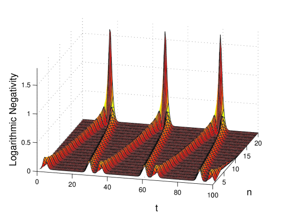
Figure 5: Same as Fig. 4 showing as well propagation of entanglement along the output arms between oscillator in the same position of each arm. $M_{\rm in}=2,M_{\rm out}=20$, $c=0.2$ and $z=10$.

Perfect transmission means that any dispersion has been reversed in the system at $t=\pi/c$ and all the supplied energy is accumulated in the two oscillators, one at each end of the outgoing arms $A$ and $B$, with the remaining oscillators in the ground state. Therefore this final joint state with $4\times 4$ covariance matrix $\gamma_{AB}=\gamma_{A}\oplus\gamma_{B}$ is pure, which is witnessed by the following equality Eisert P 03

$$-[\gamma_{AB}(t=\pi/c)\sigma]^{2}={\sf 1\rule[0.04303pt]{0.51663pt}{6.54443pt}\rule[0.04303pt]{1.29167pt}{0.51663pt}},$$ (25)

where $\sigma$ is the $4\times 4$ symplectic matrix given by

$$\sigma=\left[\begin{array}[]{cccccc}0&{{\sf 1\rule[0.04303pt]{0.51663pt}{6.54443pt}\rule[0.04303pt]{1.29167pt}{0.51663pt}}}_{2}\\ -{{\sf 1\rule[0.04303pt]{0.51663pt}{6.54443pt}\rule[0.04303pt]{1.29167pt}{0.51663pt}}}_{2}&0\end{array}\right].$$ (26)

At this perfect transmission instants the evolution of the input state toward the final one $\gamma_{1}\rightarrow\gamma_{AB}$ is an unitary transformation. Its expression can be obtained by first considering the covariance matrix of the transformed system in which there is perfect transmission between initial state and A arm, while B arm is decoupled. In the new coordinates $Q,P$ (we take out the operator symbols for the sake of symplicity), the joint state of the last two oscillators in the arms $A,B$

$$\gamma_{AB}^{QP}=\left[\begin{array}[]{ccccccc}\langle{Q^{A}}^{2}\rangle&\langle Q^{A}P^{A}\rangle&0&0\\ \langle P^{A}Q^{A}\rangle&\langle{P^{A}}^{2}\rangle&0&0\\ 0&0&\langle{Q^{B}}^{2}\rangle&\langle Q^{B}P^{B}\rangle\\ 0&0&\langle P^{B}Q^{B}\rangle&\langle{P^{B}}^{2}\rangle\end{array}\right],$$ (27)

must therefore equal the direct sum of the squeezed initial state (perfect transmission with A arm) and the ground state (decoupled B arm )

$$\gamma_{AB}^{QP}=\gamma_{1{\sf 1\rule[0.03012pt]{0.36165pt}{4.58112pt}\rule[0.03012pt]{0.90417pt}{0.36165pt}}}=\gamma_{1}\oplus\gamma_{\sf 1\rule[0.03012pt]{0.36165pt}{4.58112pt}\rule[0.03012pt]{0.90417pt}{0.36165pt}}=\left[\begin{array}[]{ccccccc}z&0&0&0\\ 0&1/z&0&0\\ 0&0&1&0\\ 0&0&0&1\end{array}\right].$$ (28)

Comparing the two matrices in Eqs. (27) and (28) we then find

$$\langle{Q^{A}}^{2}\rangle = z,\;\;\langle{P^{A}}^{2}\rangle=1/z,\;\;\langle{Q^{B}}^{2}\rangle=\langle{P^{B}}^{2}\rangle=1$$

$$\langle Q^{A}P^{A}\rangle = \langle P^{A}Q^{A}\rangle=\langle Q^{B}P^{B}\rangle=\langle P^{B}Q^{B}\rangle=0.$$ (29)

The covariance matrix of the output oscillators in both arms of the original coupled Y-shaped structure

$$\gamma_{AB}^{qp}=\gamma_{A}\oplus\gamma_{B}=\left[\begin{array}[]{ccccccc}\langle{q^{A}}^{2}\rangle&\langle q^{A}p^{A}\rangle&0&0\\ \langle p^{A}q^{A}\rangle&\langle{p^{A}}^{2}\rangle&0&0\\ 0&0&\langle{q^{B}}^{2}\rangle&\langle q^{B}p^{B}\rangle\\ 0&0&\langle p^{B}q^{B}\rangle&\langle{p^{B}}^{2}\rangle\end{array}\right],$$ (30)

can then be obtained by applying (24). Taking into account the symmetry ($\gamma_{A}=\gamma_{B}$) to notice that $\langle Q^{A}Q^{B}\rangle=\langle P^{A}P^{B}\rangle=\langle Q^{A}P^{B}+Q^{B}P^{A}\rangle=0$, and with Eqs. (29) we find

$$\gamma_{AB}=\gamma_{A}\oplus\gamma_{B}=\frac{1}{2}\left[\begin{array}[]{ccccccc}z+1&0&0&0\\ 0&1/z+1&0&0\\ 0&0&z+1&0\\ 0&0&0&1/z+1\end{array}\right].$$ (31)

This finally leads to the transformation mapping the initial into the final state for the Y-shape given by

$$\gamma_{A}(t=\pi/c)=\gamma_{B}(t=\pi/c)=\frac{1}{2}[\gamma_{1}(t=0)+{\sf 1\rule[0.04303pt]{0.51663pt}{6.54443pt}\rule[0.04303pt]{1.29167pt}{0.51663pt}}]$$ (32)

For these pure states we can use entropy of entanglement Eq.(9) as a good measure of entanglement Eisert P 03 ; Plenio V 05 . To obtain the dependence of $\mu_{1}$ with the squeezing parameter we need to determine the positive eigenvalues of the matrix Audenaert EPW 02

$$B=-i\sigma\gamma_{A},$$ (33)

where $\sigma$ is the symplectic matrix (26). We introduce Eq. (32) (with $\gamma_{1}$ given by (20)) in Eq. (33), and take just the positive one of the two real conjugated eigenvalues of $B$

$$\mu_{1}=\frac{1}{2}\sqrt{z+1/z+2},$$ (34)

which can be introduced in (9) with $m=1$ to obtain the expression $S(z)$.

It is interesting now to compare the obtained entanglement to the largest possible entanglement the system can yield given the total energy $E_{T}(z)$ that have been supplied through squeezing of the input oscillator

$$E_{T}(z)=\frac{1}{2}({\langle q_{1}^{2}\rangle}+{\langle p_{1}^{2}\rangle})-1=\frac{1}{2}(z+1/z)-1,$$ (35)

where the $-1$ stands for a shift in energy such that the energy of coherent states be zero, $E_{T}(z=1)=0$. Therefore we want to maximize entropy of entanglement

$$S(\rho_{A})=-\mbox{tr}(\rho_{A}\log\rho_{A})=-\sum_{i=1}^{\infty}\lambda_{i}\log\lambda_{i},$$ (36)

with the following constraints for probability and energy conservation

$$\mbox{tr}(\rho_{A}) = \sum_{i=1}^{\infty}\lambda_{i}=1$$ (37)

$$\mbox{tr}(\rho H) = \sum_{i=1}^{\infty}\lambda_{i}2E_{i}=E_{T}(z).$$ (38)

The $\lambda_{i}$ are the Schmidt coefficients of the density matrix $\rho=\sum_{i=1}^{\infty}\lambda_{i}|i\rangle\langle i|$ (where we have taken into account symmetry between particles, i.e. $|i_{A}\rangle=|i_{B}\rangle=|i\rangle$), and $E_{i}=i$ are the dimensionless eigenstates of one harmonic oscillator. Using Lagrange multipliers we obtain the maximum entanglement the system can yield in terms of the squeezing parameter $z$

$$S_{max}(\rho_{A})=\frac{1}{\mbox{ln}2}\left[\frac{E_{T}(z)}{2}\mbox{ln}\left(\frac{2}{E_{T}(z)}+1\right)\right.\\ +\left.\mbox{ln}\left(\frac{E_{T}(z)}{2}+1\right)\right],$$ (39)

where the total energy is given by Eq. (35). Fig. 6 shows the obtained entanglement (maximum in time evolution) in the Y-shaped structure, Eq. (9), and the maximum one, Eq. (39), in terms of $z$. Both quantities are independent on the coupling constant $c$ and on the number of oscillators.

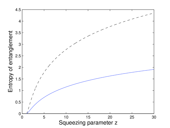
Figure 6: (Solid line) Entanglement obtained in the Y-shaped structure between the oscillators in the extremes of the output arms (maximum at $t=\pi/c$) and (dashed line) maximum entanglement in the system given a energy $E(z)$, vs. squeezing parameter $z$.

III.2 Multipartite entanglement

The arguments presented above can be extended easily to a structure in which one has $N_{A}$ output arms structure as depicted in Fig. 7 (see McAneney PK 05 for a treatment of similar structures).

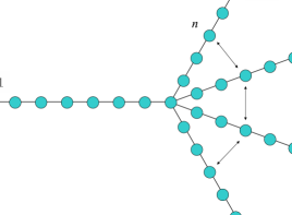
Figure 7: Multiarm structure for $N_{A}=4$, $M_{\rm in}=8$ and $M_{\rm out}=5$. Arrows indicates how to group oscillators in the same position $n$ of each branch to apply DFT basis change (41).

Now the coupling in the junction, Eq. (23), must be

$$V_{M_{\rm in},M_{\rm in}+1}=\frac{c}{2}\sqrt{n(M-n)/N_{A}},$$ (40)

and the basis change which decouples all arms except one (for which perfect transmission is obtained) is now a discrete Fourier transform (DFT). We apply it to position ${\hat{q}}_{n}^{k}$ and momentum ${\hat{p}}_{n}^{k}$ operators of oscillators occupying the same position $n$ in each arm (see Fig. 7) to obtain the new basis operators

$${\hat{Q}}_{n}^{j}=\frac{1}{\sqrt{N_{A}}}\sum_{k=1}^{N_{A}-1}{\hat{q}}_{n}^{k}e^{2\pi ijk/N_{A}},$$ (41)

with an analogous expression for momentum operators. We can now follow the same procedure that yielded Eq. (32) to obtain the unitary transformation which links initial squeezed state in the input oscillator with the final state at $t=\pi/c$ of the last oscillator in one of the $N_{A}$ arms

$$\gamma_{A}(t=\pi/c)=\frac{1}{N_{A}}[\gamma_{1}(t=0)+(N_{A}-1){\sf 1\rule[0.04303pt]{0.51663pt}{6.54443pt}\rule[0.04303pt]{1.29167pt}{0.51663pt}})].$$ (42)

which reduces to Eq. (32) for $N_{A}=2$. The initial state is distributed between $N_{A}$ final states and we compute multipartite entanglement as the bipartite entanglement between the oscillator in the extreme of one arm and the other oscillators in the rest of arms. Following the same procedure to obtain Eq. (34) we can get now the positive symplectic eigenvalue of the reduce covariance matrix in the multiarm structure

$$\mu_{1}(N_{A})=\frac{1}{N_{A}}\sqrt{(z+N_{A}-1)(1/z+N_{A}-1)},$$ (43)

which it is introduced in Eq. (9) to obtain the expected behaviour shown in Fig. 8: multipartite entanglement decreases with increasing number of arms.

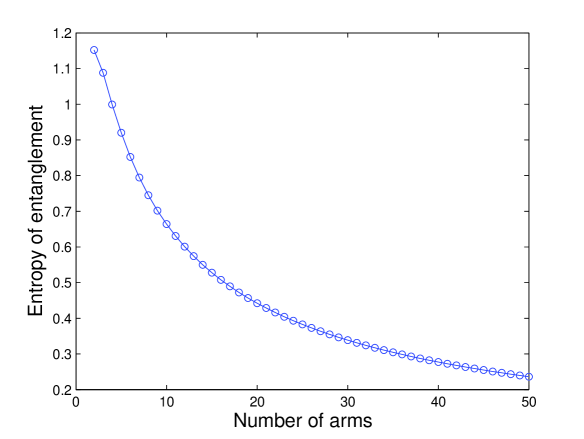
Figure 8: Multipartite entanglement obtained in the multiarm structure (maximum in entanglement evolution at $t=\pi/c$) vs. the number of arms $N_{A}$.

III.3 Beamsplitters

Extending arguments of previous section we now study X-shaped arrays. Such structures may be used to split the entanglement in a state. In qubit systems, entanglement splitting cannot be achieved without loss Buzek VPKH 97 but we will see that the Gaussian setting permits lossless splitting.

To obtain the equivalent perfect transmission, coupling strengths must be adjusted analogously to the Y-shaped case, Eqs. (21, 22), but with an interaction applied to the coupling between the central oscillator and its four nearest neighbours given by

$$V_{M_{\rm in-1},M_{\rm in}}=V_{M_{\rm in},M_{\rm in}+1}=\frac{c}{2}\sqrt{M_{\rm in}(M-M_{\rm in})}.$$ (44)

As initial condition we now create an entangled two-mode squeezed state between the first two oscillators in the input arm, labelled with $1,2$

$$\gamma_{q_{1}q_{1}} = \gamma_{q_{2}q_{2}}=\gamma_{p_{1}p_{1}}=\gamma_{p_{2}p_{2}}=\cosh(r)$$

$$\gamma_{q_{1}q_{2}} = -\gamma_{p_{1}p_{2}}=\sinh(r),$$ (45)

with $\cosh(r)=z$. The resulting time-space evolution of entanglement is shown in Figs. 10, 11, and we sketch an explanation for the observed patterns in the caption of Fig. 9.

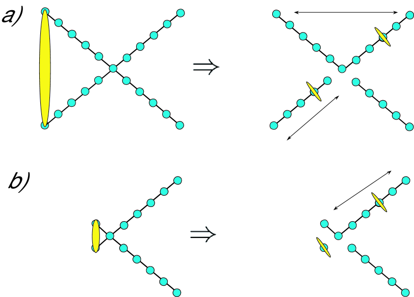
Figure 9: a) Under the transformation Eq. (24) the X-shape on the left hand side is transformed into a linear chain and two decoupled arms. The initial two mode squeezed state (represented by the yellow disk across two arms) is then transformed into a tensor product of two single mode squeezed states (individual yellow disks) . One of these can move through all the structure, while the other one remains in the input arm, giving rise to the complex time-space pattern shown in Fig. 10. b) When there is just one oscillator in the input arm, one of the states always remains in the first oscillator and entanglement is always present in the input arm as shown in Fig. 11

.

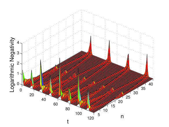
Figure 10: Time-space evolution of entanglement in the X-shaped structure. For times when one of the squeezed states is in the output arm, regular transmission patterns are obtained because the other one must stay in the input arm. (see Fig. 9a). However when the state returns to the input arm irregular patterns are obtained as now both states are in the input arms. Maximum entanglement is obtained when both squeezed states are in the input oscillator.

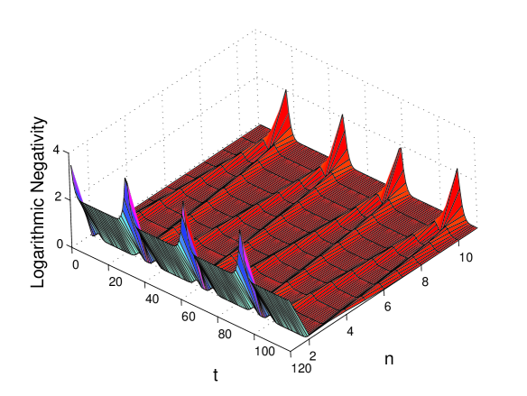
Figure 11: Time-space evolution of entanglement in the X-shaped structure when there is just one oscillatr in the input arm (see Fig. 9b). There is always entanglement between the two oscillators in the input arm as one of the squeezed states remains always in it.

IV Cloning

At the times when perfect transmission is obtained adjusting the couplings, the states at the end of both arms can be considered as approximate copies of the input states. However, we must be careful to adjust the diagonal element of the $V$ and $T$ matrices to optimize quality of the clones as the local rotation of the individual oscillators must now be taken into account. The reason is that we are now comparing actual quantum states at different times, $\rho_{1}(t=0)$ and $\rho_{A}(t=\pi/c)$, while in entanglement calculation the local rotations did not affect the amount of entanglement. We find that in Eq. (22) we must modify diagonal elements in the following way

$$V_{n,n}=\left\{\begin{array}[]{cccccc}c/2&\mbox{for}&\;\;\;M_{\rm in}+M_{\rm out}\;\;\;\mbox{even}\\ c&\mbox{for}&\;\;\;M_{\rm in}+M_{\rm out}\;\;\;\mbox{odd}\end{array}\right.,$$ (46)

which can be expressed as

$$V_{n,n}=\frac{1}{4}[3-(-1)^{(M_{\rm in}+M_{\rm out})}]c.$$ (47)

It is worthwhile pointing out that with these and any other arbitrary value for the diagonal elements we also obtain optimum entanglement creation, as internal degrees of freedom are equal for botharms and henceforth entanglement is not affected.

The fidelity between the pure input state $\rho_{1}$ and one of the two copies, described by the reduced density operator $\rho_{A}$, is given by

$$F=\langle\Psi_{1}|\rho_{A}|\Psi_{1}\rangle=\mbox{tr}(\rho_{1}\rho_{A}).$$ (48)

We now insert in this expression the input state $\rho_{1}=|\Psi_{1}\rangle\langle\Psi_{1}|$ given by Eq. (5), and consider no displacement ($d=0$) and initial state $\chi_{\rho}(0)$ equal to one in Eq. (6). Using expression (4) and solving the resulting Gaussian integral we obtain

$$F(\gamma_{1},\gamma_{A})=\frac{2}{\sqrt{\mbox{det}(\gamma_{1}+\gamma_{A})}},$$ (49)

where $\gamma_{1}$ as the initial covariance matrix of the input oscillator (20), and $\gamma_{A}$ is the final one at $t=\pi/c$ of the A-arm output oscillator ($\gamma_{A}=\gamma_{B}$ for symmetry).

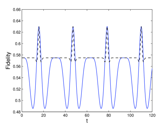
Figure 12: Time evolution of fidelity between initial squeezed state in the first oscillator in the input arm and final state in the last oscillator of the output arm in the Y-shaped structure. Maximum fidelity is obtained for $t=\pi/c$. Solid line corresponds to $M_{\rm in}=M_{\rm out}=2$ and dashed line to $M_{\rm in}=M_{\rm out}=20$. $c=0.2$ and $z=10$.

In Fig. 12 the fidelity time evolution is shown. The value $F\approx 0.575$ corresponds to overlap between input squeezed state $\gamma_{q_{1}q_{1}}=1/\gamma_{p_{1}p_{1}}=z$ and ground state $\gamma_{A}={\sf 1\rule[0.04303pt]{0.51663pt}{6.54443pt}\rule[0.04303pt]{1.29167pt}{0.51663pt}}$. At the same time for which we obtained perfect transmission and maximum entanglement, $t=\pi/c$, we obtain as well maximum fidelity. At this times rest of oscillators are at ground states and relation (32) between covariance matrices of input and output oscillators holds. If we insert this relation in Eq. (49) and express $\gamma_{1}$ elements in terms of the squeezing parameter $z$, Eq. 20, we get

$$F(z)=\frac{4}{\sqrt{3z+3/z+10}},$$ (50)

which is depicted in Fig. 13. For $z=1$ we have a ground state as input and a ground state as output and so the maximum is reached at $F(1)=1$ and fidelity decreases as squeezing is increased.

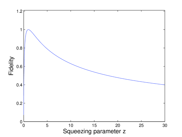
Figure 13: Fidelity obtained in the Y-shaped structure between the first oscillator in the input arm and the last oscillator in the extreme of one of the output arms (maximum at $t=\pi/c$), vs. squeezing parameter $z$.

In the $N_{A}$ multiarm structure the fidelity can be calculated inserting the unitary transformation (42) in the fidelity expression (49) to get

$$F(z,N_{A})=\frac{2N_{A}}{\sqrt{(N_{A}^{2}-1)(z+1/z)+2N_{A}^{2}+2}},$$ (51)

which reduces to Eq. (50) for $N_{A}=2$. In Fig. 14 we can see that with increasing number of arms we obtain a faster decreasing of fidelity than the one obtained for entanglement. For $N_{A}\rightarrow\infty$ fidelity approaches the value $F\approx 0.575$ which corresponds to an initial state with $z=10$ and a final ground state.

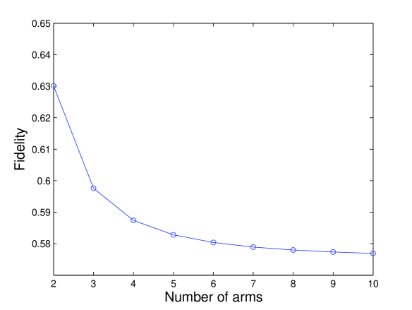
Figure 14: Fidelity in a 1 to $N_{A}$ cloner obtained in the multiarm structure (maximum in fidelity evolution at $t=\pi/c$) vs. the number of arms $N_{A}$, for $z=10$.

V Conclusions

We have considered situations in which we propagate quantum information through a system of interacting quantum systems such that, in the course of this propagation, it suffers a non-trivial quantum state transformation. In particular we have considered entanglement creation, quantum cloning and entanglement splitting in systems of quantum harmonic oscillators both analytically and numerically under the rotating wave approximation (RWA) as it is appropriate in a quantum optical setting.

We have presented geometrical structures that allow to create, by propagation, the complex unitary operations required for the above processes. Such hard wired pre-fabricated structures may also be ’programmable’ by external actions to add further functionality to them. Therefore quantum information would be manipulated through its propagation in these devices somewhat analogous to modern micro-chips and as opposed the most presently suggested implementations of quantum information processing where stationary quantum bits are manipulated by a sequence of external interventions such as laser pulses.

All these investigations were deliberately left at a device independent level. It should nevertheless be noted that there are many possible realizations of the above phenomena. These include nano-mechanical oscillators Eisert PBH 03 , arrays of coupled atom-cavity systems, photonic crystals, and many other realizations of weakly coupled harmonic systems, potentially even vibrational modes of molecules in molecular quantum computing Tesch R 02 . We hope that these ideas may lead to the development of novel ways for the implementation of quantum information processing in which the quantum information is manipulated by flowing through pre-fabricated circuits that can be manipulated from outside.

Acknowledgements: Support by a Royal Society Incoming Visitors award is gratefully acknowledged. This work is part of the QIP-IRC (www.qipirc.org) supported by EPSRC (GR/S82176/0) and has also been supported by the EU Thematic Network QUPRODIS (IST-2001-38877), the Leverhulme Trust grant F/07 058/U and Project UAH-PI12005/68 of the University of Alcalá.

References

- (1) J. Eisert and M.B. Plenio, Int. J. Quant. Inf. 1, (2003).
- (2) J. Eisert, M.B. Plenio, S. Bose and J. Hartley, Phys. Rev. Lett. 93, 190402 (2004)
- (3) M.B. Plenio, J. Hartley and J. Eisert, New J. Phys. 6, 36 (2004).
- (4) M.B. Plenio and F. Semião, New J. Phys. 7, 73 (2005).
- (5) H. McAneney, M. Paternostro and M.S. Kim, Phys. Rev. Lett. 94, 070501 (2005).
- (6) M. Paternostro, M.S. Kim, E. Park, and J. Lee, E-print arxiv quant-ph/0506148.
- (7) M.-H. Yung and S. Bose, Phys. Rev A 71, 032310 (2005)
- (8) C. Hadley, A. Serafini and S. Bose, E-print arxive quant-ph/0507274
- (9) R. Simon, E.C.G. Sudarshan, and N. Mukunda, Phys. Rev. A 36, 3868 (1987).
- (10) K. Audenaert, J. Eisert, M.B. Plenio, and R.F. Werner, Phys. Rev. A 66, 042327 (2002).
- (11) K. Audenaert, M.B. Plenio, and J. Eisert, Phys. Rev. Lett. 90, 027901 (2003).
- (12) K. Zyczkowski, P. Horodecki, A. Sanpera, and M. Lewenstein, Phys. Rev. A 58, 883 (1998).
- (13) J. Eisert and M.B. Plenio, J. Mod. Opt. 46, 145 (1999).
- (14) G. Vidal and R.F. Werner, Phys. Rev. A 65, 32314 (2002).
- (15) J. Lee, M.S. Kim, Y.J. Park, and S. Lee, J. Mod. Opt. 47, 2151 (2000).
- (16) J. Eisert, PhD thesis, Potsdam, February 2001.
- (17) M.B. Plenio, Phys. Rev. Lett. 95, 090503 (2005).
- (18) M.B. Plenio and S. Virmani, E-print arXiv quant-ph/0504163
- (19) M.M. Wolf, J. Eisert, and M.B. Plenio, Phys. Rev. Lett. 90, 047904 (2003).
- (20) M.B. Plenio, J. Eisert, J. Dreiig and M. Cramer, Phys. Rev. Lett. 95, 060503 (2005).
- (21) M. Christandl, N. Datta, A. Ekert, A.J. Landahl, LANL e-print quant-ph/0309131.
- (22) V. Buzek, V. Vedral, M.B. Plenio, P.L. Knight and M. Hillery, Phys. Rev. A 55, 3327 (1997).
- (23) C.M. Tesch and R. de Vivie-Riedle, Phys. Rev. Lett. 89, 157901 (2002).