Single-passage read-out of atomic quantum memory

Abstract

A scheme for retrieving quantum information stored in collective atomic spin systems onto optical pulses is presented. Two off-resonant light pulses cross the atomic medium in two orthogonal directions and are interferometrically recombined in such a way that one of the outputs carries most of the information stored in the medium. In contrast to previous schemes our approach requires neither multiple passes through the medium nor feedback on the light after passing the sample which makes the scheme very efficient. The price for that is some added noise which is however small enough for the method to beat the classical limits.

I Introduction

The development of complex quantum communication networks requires the interface between light and atomic carriers of quantum information. The photons are ideal for transmitting the quantum information over long distances. The atoms, on the other hand, are optimally suited for local storage of quantum states in the internal ground-state coherences which can exhibit very long life-time. Ideally, the atoms should form a quantum memory for light where the quantum state of the optical beam can be stored, possibly processed, and retrieved later on in a controlled manner. The quantum memory is an essential ingredient of quantum repeaters Briegel98 ; Duan01 that allow for long-distance quantum communication over realistic noisy quantum channels and it is also necessary for scalable all-optical quantum computing as proposed by Knill, Laflamme and Milburn Knill01 .

Several methods for exchanging the quantum states of light and atoms have been considered in the literature such as storing the state of a single photon in a single atom Cirac97 or coupling the light to an ensemble of atoms Kuzmich97 ; Hald99 ; Duan01 ; Kuzmich00 ; Kozhekin00 ; Julsgaard04 ; Kuzmich04 ; Dantan05 . The latter approach seems to be particularly advantageous because it is not necessary to employ a cavity and work in the strong coupling regime. Instead sufficiently strong interaction is achieved due to the collective enhancement effect Julsgaard01 ; Geremia04 . An alternative to direct light-matter state exchange is to first prepare an entangled state of atoms and light and then teleport the quantum state of light onto atoms. The entanglement between a photon and a single trapped ion has been reported Blinov04 and also entanglement between a photon and an ensemble of atoms has been observed Kuzmich04 . In related experiments, correlated photon pairs emitted by an atomic ensemble were detected Wal03 ; Kuzmich03 ; Chou04 .

The storage of a quantum state of light mode in the ensemble of atoms has been recently demonstrated experimentally Julsgaard04 by exploiting the off-resonant interaction of light with a cloud of cesium atoms held in a glass cell at room temperature Kuzmich98 ; Kuzmich00a ; Duan00 ; Julsgaard01 ; Schori02 . In that experiment, weak coherent states were stored for a few milliseconds and the fidelity of the stored states exceeded the best fidelity achievable by a classical measure-and-prepare procedure. The storage protocol consisted of sending the light beam through the atomic ensemble, performing a suitable measurement on the outgoing light and applying an appropriate feedback on atoms with the help of a magnetic field. This procedure, however, cannot be directly inverted to retrieve the quantum state from atoms back onto light due to the current technical limitations. The light pulses used in the experiment need to be about 1 ms long (i.e. $300$ km) and the memory readout would require storing somewhere the first pulse which interacted with the atomic ensemble while a second auxiliary light beam is used to measure the atoms. The required long duration of the pulses also prevents one to employ measurement-free retrieval methods based on multiple passages of the light pulse through the atomic sample Kuzmich03b ; Fiurasek03 ; Hammerer04 .

A possible solution to these problems has been suggested by using two- and four-pass protocols with the light beam crossing the medium simultaneously from two perpendicular directions Sherson05 . Although high fidelity readout can theoretically be achieved in these protocols they each suffer from deficiencies which can decrease their general applicability. The two-pass protocol is asymmetric with respect to the two conjugate quadratures and a unity gain readout is difficult to achieve since it would require a complicated temporal profile of the coupling light beam. This makes the two-pass protocol unsuitable for readout of general input states. With the four-pass protocol perfect readout can be achieved in principle, however, since it involves so many passages even a small light reflection loss at each crossing can seriously decrease the achievable fidelities. This point will be investigated quantitatively for our protocol below.

In this paper we suggest an alternative protocol for read-out of the atomic quantum memory which requires only a single passage of the light through the atoms and is therefore rather robust with respect to losses on the glass cell walls. The simultaneous transfer of both atomic quadratures $x_{A}$ and $p_{A}$ onto light is achieved by sending two light beams perpendicularly to each other through the memory unit, see Fig. 1. The scheme can be explained on the simplified model with a single atomic ensemble as in Fig. 1a, however, to avoid technical noises, experiments are usually done using two cells in external magnetic field (see Fig. 1b), observing the phenomena on the sidebands of the light pulses. As it turns out, these two approaches yield similar results, however, the number of crosses of the beams through the cell walls plays a crucial role in increasing the noise.

The rest of the paper is organized as follows. In Section II we derive the formula for the output light quadratures and the readout fidelity. In Section III we take into account the effect of losses and show how they influence the read-out fidelity in both the single-cell and double-cell schemes. We will also demonstrate that the readout can be improved by squeezing the input light beams entering the cell. Finally, Section IV contains brief conclusions.

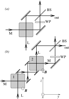
Figure 1: Scheme for the single-passage read-out of the atomic quantum memory. Two light beams L and M simultaneously pass through one $(a)$ or two $(b)$ atomic ensembles. The wave plate (WP) swaps the quadratures $x$ and $p$ in one of the beams. Afterwords, the beams are (re)combined on a balanced beam splitter BS.

II Readout protocol

II.1 Single-cell scheme

Let us first deal with the single-cell scheme with no magnetic field. The beam L propagates along the $z$ axis and the Hamiltonian describing its coupling with the atomic ensemble is $H_{L}=aS^{L}_{3}J_{z}$ and the second beam M propagates along the $y$ axis and interacts with the ensemble according to $H_{M}=aS^{M}_{3}J_{y}$ so that the complete Hamiltonian is

$$H=a\left(S^{L}_{3}J_{z}+S^{M}_{3}J_{y}\right).$$ (1)

Here $\bm{S}$ denotes the Stokes vector characterizing the polarization properties of a light beam, $\bm{J}$ stands for the collective atomic spin operator and $a$ is the coupling constant Kuzmich98 ; Kuzmich00 ; Duan00 . The orientation of the Stokes vectors is chosen such that $S_{3}$ describes the helicity and $S_{1}$ describes linear polarization, with positive $S_{1}$ corresponding to $x$-polarized light. The components of $\bm{S}$ and $\bm{J}$ satisfy the angular momentum-type commutation relations, $[J_{j},J_{k}]=i\epsilon_{jkl}J_{l}$ with $j,k,l\in\{x,y,z\}$ and $[S^{L}_{j}(t),S^{L}_{k}(t^{\prime})]=i\epsilon_{jkl}\delta(t-t^{\prime})S^{L}_{l}(t)$, and $[S^{M}_{j}(t),S^{M}_{k}(t^{\prime})]=i\epsilon_{jkl}\delta(t-t^{\prime})S^{M}_{l}(t)$ with $j,k,l\in\{1,2,3\}$.

Both beams M and L contain strong $x$ polarized component such that the $S_{1}$ components of the Stokes vectors $S^{L}_{1}(t)$ and $S^{M}_{1}(t)$ can be approximated by c-numbers. We assume that the $S_{1}$ components are constant throughout the duration of the pulses and both beams have the same intensity,

$$S^{L}_{1}(t)=S^{M}_{1}(t)=\frac{N_{L}}{2T}\equiv S_{1},$$ (2)

where $N_{L}$ is the total number of photons in the strong component of each beam and $T$ is the duration of the pulse. Similarly, the atoms are polarized along the $x$ axis and the $x$ component of the collective atomic spin attains a macroscopic value and the operator $J_{x}$ can be replaced with a c-number, $J_{x}\approx\langle J_{x}\rangle$.

In the Heisenberg picture, the atomic quadratures evolve according to

$$\frac{dJ_{y}}{dt}=a\langle J_{x}\rangle S^{L}_{3}(t),\qquad\frac{dJ_{z}}{dt}=-a\langle J_{x}\rangle S^{M}_{3}(t).$$ (3)

The relations between input and output $y$ and $z$ components of the Stokes vectors of beams L and M read Schori02 ,

$$S_{2}^{L,{\rm out}}(t) = S_{2}^{L,\rm in}(t)+aS_{1}J_{z}(t),$$

$$S_{3}^{L,\rm out}(t) = S_{3}^{L,\rm in}(t),$$

$$S_{2}^{M,\rm out}(t) = S_{2}^{M,\rm in}(t)+aS_{1}J_{y}(t),$$

$$S_{3}^{M,\rm out}(t) = S_{3}^{M,\rm in}(t).$$ (4)

The Heisenberg equations (3) can be easily solved and yield

$$J_{y}(t)=J_{y}(0)+a\langle J_{x}\rangle\int_{0}^{t}S^{L}_{3}(\tau)d\tau,$$

$$J_{z}(t)=J_{z}(0)-a\langle J_{x}\rangle\int_{0}^{t}S^{M}_{3}(\tau)d\tau.$$ (5)

We define the quadratures of the light modes L and M in the usual way as integrals over the whole pulse,

$$x_{L,M} = \sqrt{\frac{2}{N_{L}}}\int_{0}^{T}S^{L,M}_{2}(t)dt,$$

$$p_{L,M} = \sqrt{\frac{2}{N_{L}}}\int_{0}^{T}S^{L,M}_{3}(t)dt.$$ (6)

We also define the atomic quadrature operators $x_{A}=J_{y}/\sqrt{\langle J_{x}\rangle},$ $p_{A}=J_{z}/\sqrt{\langle J_{x}\rangle}$. All these operators satisfy the canonical commutation relations $[x_{j},p_{k}]=i\delta_{jk}$. Upon combining the equations (4), (5) and (6) and changing the order of integration we obtain the expression for $x_{L}^{\rm out}$,

$$x_{L}^{\rm out}=x_{L}^{\rm in}+\kappa p_{A}^{\rm in}-\kappa^{2}\int_{0}^{T}dt\left(1-\frac{t}{T}\right)\frac{S^{M}_{3}(t)}{\sqrt{N_{L}/2}},$$ (7)

where we introduced the effective coupling constant $\kappa=a\sqrt{N_{L}\langle J_{x}\rangle/2}$. We can see that the description in terms of the light modes (6) is incomplete because a mode with non-constant temporal profile $1-t/T$ couples to $x_{L}^{\rm out}$. The two mode profiles we are dealing with are

$$f_{1}(t)=1,\qquad f_{2}(t)=\sqrt{3}\left(1-\frac{t}{T}\right),$$ (8)

with the normalization $\int_{0}^{T}|f_{j}^{2}(t)|dt=T$. The two mode functions (8) are not orthogonal since $\int_{0}^{T}f_{1}(t)f_{2}(t)dt=T\sqrt{3}/2$. We can decompose $f_{2}(t)$ as follows,

$$f_{2}(t)=\frac{\sqrt{3}}{2}f_{1}(t)+\frac{1}{2}f_{3}(t),$$ (9)

where $f_{3}(t)=\sqrt{3}(1-2t/T)$ and the functions $f_{1}(t)$ and $f_{3}(t)$ are now orthogonal.We define quadrature operators corresponding to the modal profile $f_{3}(t)$,

$$\tilde{x}_{L,M} = \sqrt{\frac{6}{N_{L}}}\int_{0}^{T}\left(1-\frac{2t}{T}\right)S^{L,M}_{2}(t)dt,$$

$$\tilde{p}_{L,M} = \sqrt{\frac{6}{N_{L}}}\int_{0}^{T}\left(1-\frac{2t}{T}\right)S^{L,M}_{3}(t)dt.$$ (10)

One can easily check that the quadratures (10) satisfy canonical commutation relations.

Using the above definitions we can express the output quadrature operator $x_{L}^{\mathrm{out}}$ as a linear combination of the input light and atomic quadrature operators. This procedure can be repeated for other quadratures and after some algebra we finally get:

$$x_{L}^{\rm out} = x_{L}^{\rm in}+\kappa p_{A}^{\rm in}-\frac{\kappa^{2}}{2}p_{M}^{\rm in}-\frac{\kappa^{2}}{2\sqrt{3}}\tilde{p}_{M}^{\rm in},$$

$$p_{L}^{\rm out} = p_{L}^{\rm in},$$

$$x_{M}^{\rm out} = x_{M}^{\rm in}+\kappa x_{A}^{\rm in}+\frac{\kappa^{2}}{2}p_{L}^{\rm in}+\frac{\kappa^{2}}{2\sqrt{3}}\tilde{p}_{L}^{\rm in},$$

$$p_{M}^{\rm out} = p_{M}^{\rm in},$$

$$x_{A}^{\rm out} = x_{A}^{\rm in}+\kappa p_{L}^{\rm in},$$

$$p_{A}^{\rm out} = p_{A}^{\rm in}-\kappa p_{M}^{\rm in}.$$ (11)

Note that the information about the $x_{A}$ and $p_{A}$ quadratures is stored in two different modes L and M. In order to obtain a single mode that would contain an approximate version of the state stored originally in the atomic memory, we have to combine the modes L and M. To accomplish this, we suggest placing a wave plate to one of the beams, say M, to switch the quadratures $x_{M}\to p_{M}$, $p_{M}\to-x_{M}$, and to let these modes interfere on a balanced beam splitter, as shown in Fig. 1. In one of the output arms we finally obtain a mode with quadratures

$$x=\frac{1}{\sqrt{2}}(x_{L}^{\rm out}+p_{M}^{\rm out}),\qquad p=\frac{1}{\sqrt{2}}(p_{L}^{\rm out}-x_{M}^{\rm out}).$$ (12)

On inserting the formulas (11) into (12), we find

$$x=\frac{\kappa}{\sqrt{2}}p_{A}^{\rm in}+\frac{1}{\sqrt{2}}x_{L}^{\rm in}-\frac{1}{\sqrt{2}}(\frac{\kappa^{2}}{2}-1)p_{M}^{\rm in}-\frac{\kappa^{2}}{2\sqrt{6}}\tilde{p}_{M}^{\rm in},$$

$$p=-\frac{\kappa}{\sqrt{2}}x_{A}^{\rm in}-\frac{1}{\sqrt{2}}x_{M}^{\rm in}-\frac{1}{\sqrt{2}}(\frac{\kappa^{2}}{2}-1)p_{L}^{\rm in}-\frac{\kappa^{2}}{2\sqrt{6}}\tilde{p}_{L}^{\rm in}.$$

(13)

If we choose $\kappa=\sqrt{2}$, then the quadratures are transfered from the atomic memory to the light mode with unit gain,

$$x = p_{A}^{\rm in}+\frac{1}{\sqrt{2}}x_{L}^{\rm in}-\frac{1}{\sqrt{6}}\tilde{p}_{M}^{\rm in},$$

$$p = -x_{A}^{\rm in}-\frac{1}{\sqrt{2}}x_{M}^{\rm in}-\frac{1}{\sqrt{6}}\tilde{p}_{L}^{\rm in}.$$ (14)

This is the main result of this paper.

The memory read-out is not perfect due to the noise of the light quadrature operators in Eq. (14). To be specific, let us consider a readout of a coherent state $|\alpha\rangle$ stored in the atomic ensemble. If the light modes are initially in vacuum states, then the added noise is the same for both quadratures and can be expressed in terms of the mean photon number $\bar{n}$ of thermal light with the same quadrature fluctuations

$$\bar{n}=\frac{1}{2}\times\left(\frac{1}{2}+\frac{1}{6}\right)=\frac{1}{3}.$$ (15)

The fidelity of the memory read-out is in this case

$$\mathcal{F}=\frac{1}{1+\bar{n}}$$ (16)

and for $\bar{n}=1/3$ we get $\mathcal{F}=3/4$. This value significantly exceeds the best fidelity $\mathcal{F}_{\rm meas}=1/2$ achievable by measure and prepare procedures, which in Hammerer05 was shown to be the optimal classical storage or retrieval procedure.

Note that the readout of the memory is imperfect because a part of the information on the state remains in the memory. In particular, for $\kappa=\sqrt{2}$ the final atomic quadratures read

$$x_{A}^{\rm out}=x_{A}^{\rm in}+\sqrt{2}p_{L}^{\rm in},\qquad p_{A}^{\rm out}=p_{A}^{\rm in}-\sqrt{2}p_{M}^{\rm in}.$$ (17)

The distribution of the quantum information between the quantum memory and the output light beam suggests that the readout protocol is related to the (asymmetric) quantum cloning. Indeed, in the limit of infinitely squeezed quadratures $\tilde{p}_{L}=\tilde{p}_{M}=0$, the formulas (14) and (17) describe exactly the two clones produced by the optimal Gaussian asymmetric $1\rightarrow 2$ cloning machine for coherent states Fiurasek01 . The anti-clone (or, more precisely, the complex conjugated clone) is carried by the light beam in the auxiliary output port of the beam splitter, whose quadrature operators can be expressed as ($\kappa=\sqrt{2}$),

$$x^{\rm aux} = p_{A}^{\rm in}+\frac{1}{\sqrt{2}}x_{L}^{\rm in}-\sqrt{2}p_{M}^{\rm in}-\frac{1}{\sqrt{6}}\tilde{p}_{M}^{\rm in},$$

$$p^{\rm aux} = x_{A}^{\rm in}+\frac{1}{\sqrt{2}}x_{M}^{\rm in}+\sqrt{2}p_{L}^{\rm in}+\frac{1}{\sqrt{6}}\tilde{p}_{L}^{\rm in}.$$ (18)

II.2 Two-cell scheme

To avoid technical noises, one can work with a two-cell scheme as shown in Fig. 1b Julsgaard04 . In this model we assume magnetic field $B$ perpendicular to the two beams such that the fields in the two cells have opposite orientation. The atomic spins then rotate around the $x$-axis with the Larmor frequency $\Omega\propto B$, the direction of rotation being opposite in the two samples. The atoms interact with light on the sidebands with frequencies $\omega_{0}\pm\Omega$, where $\omega_{0}$ is the carrier frequency. The quadratures of cosine and sine modes at sideband frequency $\Omega\gg 1/T$ are defined as follows,

$$x^{C}_{L,M} = \frac{2}{\sqrt{N_{L}}}\int_{0}^{T}S_{2}^{L,M}(t)\cos(\Omega t)dt,$$

$$p^{C}_{L,M} = \frac{2}{\sqrt{N_{L}}}\int_{0}^{T}S_{3}^{L,M}(t)\cos(\Omega t)dt,$$

$$x^{S}_{L,M} = \frac{2}{\sqrt{N_{L}}}\int_{0}^{T}S_{2}^{L,M}(t)\sin(\Omega t)dt,$$

$$p^{S}_{L,M} = \frac{2}{\sqrt{N_{L}}}\int_{0}^{T}S_{3}^{L,M}(t)\sin(\Omega t)dt.$$

The quadratures $\tilde{x}_{L,M}^{C,S}$ and $\tilde{p}_{L,M}^{C,S}$ corresponding to modes with temporal profile $\sqrt{3}(1-2t/T)$ can be defined in a similar way. The interaction between light and atomic sample 1 can be described by means of the Hamiltonian

$$H^{(1)}=a(S_{3}^{L}J_{z}^{(1)}+S_{3}^{M}J_{y}^{(1)})-\Omega J_{x}^{(1)},$$ (19)

where the term proportional to $\Omega$ arises due to the applied magnetic field. The interaction between light and atomic sample 2 is then described by

$$H^{(2)}=a(S_{3}^{L}J_{z}^{(2)}+S_{3}^{M}J_{y}^{(2)})+\Omega J_{x}^{(2)}.$$ (20)

The information is encoded in the sum- or difference-quadratures of the collective atomic spins

$$x_{A\pm} = \frac{1}{\sqrt{2}}\left(x_{A}^{(1)}\pm x_{A}^{(2)}\right)$$ (21)

$$p_{A\pm} = \frac{1}{\sqrt{2}}\left(p_{A}^{(1)}\pm p_{A}^{(2)}\right).$$ (22)

The input-output relations can be derived in a similar manner as for the single-cell scheme by solving the linear Heisenberg equations of motion. In the limit $\Omega T\gg 1$ which is satisfied in the experiments ($\Omega T\approx 300$) one thus gets

$$x_{L}^{C,\rm out} = x_{L}^{C,\rm in}+\kappa p_{A+}^{\rm in}-\frac{\kappa^{2}}{2}p_{M}^{C,{\rm in}}-\frac{\kappa^{2}}{2\sqrt{3}}\tilde{p}_{M}^{C,{\rm in}},$$

$$p_{L}^{C,\rm out} = p_{L}^{C,\rm in},$$

$$x_{M}^{C,\rm out} = x_{M}^{C,\rm in}+\kappa x_{A+}^{\rm in}+\frac{\kappa^{2}}{2}p_{L}^{C,{\rm in}}+\frac{\kappa^{2}}{2\sqrt{3}}\tilde{p}_{L}^{C,{\rm in}},$$

$$p_{M}^{C,\rm out} = p_{M}^{C,\rm in},$$

$$x_{L}^{S,\rm out} = x_{L}^{S,\rm in}-\kappa x_{A-}^{\rm in}-\frac{\kappa^{2}}{2}p_{M}^{S,{\rm in}}-\frac{\kappa^{2}}{2\sqrt{3}}\tilde{p}_{M}^{S,{\rm in}},$$

$$p_{L}^{S,\rm out} = p_{L}^{S,\rm in},$$

$$x_{M}^{S,\rm out} = x_{M}^{S,\rm in}+\kappa p_{A-}^{\rm in}+\frac{\kappa^{2}}{2}p_{L}^{S,{\rm in}}+\frac{\kappa^{2}}{2\sqrt{3}}\tilde{p}_{L}^{S,{\rm in}},$$

$$p_{M}^{S,\rm out} = p_{M}^{S,\rm in},$$ (23)

for the light beams, and for the atomic samples

$$x_{A+}^{\rm out} = x_{A+}^{\rm in}+\kappa p_{L}^{C,{\rm in}},$$

$$p_{A+}^{\rm out} = p_{A+}^{\rm in}-\kappa p_{M}^{C,{\rm in}},$$

$$x_{A-}^{\rm out} = x_{A-}^{\rm in}+\kappa p_{M}^{S,{\rm in}},$$

$$p_{A-}^{\rm out} = p_{A-}^{\rm in}+\kappa p_{L}^{S,{\rm in}}.$$ (24)

So as to have the atomic quadratures in one beam, we place a quarter-wave plate in beam M, thus switching the quadratures $x_{M}^{C,S}\to p_{M}^{C,S}$ and $p_{M}^{C,S}\to-x_{M}^{C,S}$, and combine the L and M beams on a beam splitter. In one of the outputs we then find the new quadratures

$$x^{C} = \frac{\kappa}{\sqrt{2}}p_{A+}^{\rm in}+\frac{1}{\sqrt{2}}x_{L}^{C,{\rm in}}$$ (25)

$$-\frac{1}{\sqrt{2}}\left(\frac{\kappa^{2}}{2}-1\right)p_{M}^{C,{\rm in}}-\frac{\kappa^{2}}{2\sqrt{6}}\tilde{p}_{M}^{C,{\rm in}},$$

$$p^{C} = -\frac{\kappa}{\sqrt{2}}x_{A+}^{\rm in}-\frac{1}{\sqrt{2}}x_{M}^{C,{\rm in}}$$ (26)

$$-\frac{1}{\sqrt{2}}\left(\frac{\kappa^{2}}{2}-1\right)p_{L}^{C,{\rm in}}-\frac{\kappa^{2}}{2\sqrt{6}}\tilde{p}_{L}^{C,{\rm in}},$$

$$x^{S} = -\frac{\kappa}{\sqrt{2}}x_{A-}^{\rm in}+\frac{1}{\sqrt{2}}x_{L}^{S,{\rm in}}$$ (27)

$$-\frac{1}{\sqrt{2}}\left(\frac{\kappa^{2}}{2}-1\right)p_{M}^{S,{\rm in}}-\frac{\kappa^{2}}{2\sqrt{6}}\tilde{p}_{M}^{S,{\rm in}},$$

$$p^{S} = -\frac{\kappa}{\sqrt{2}}p_{A-}^{\rm in}-\frac{1}{\sqrt{2}}x_{M}^{S,{\rm in}}$$ (28)

$$-\frac{1}{\sqrt{2}}\left(\frac{\kappa^{2}}{2}-1\right)p_{L}^{S,{\rm in}}-\frac{\kappa^{2}}{2\sqrt{6}}\tilde{p}_{L}^{S,{\rm in}}.$$

If we choose $\kappa=\sqrt{2}$, the input-output relations for the light are

$$x^{C} = p_{A+}^{\rm in}+\frac{1}{\sqrt{2}}x_{L}^{C,{\rm in}}-\frac{1}{\sqrt{6}}\tilde{p}_{M}^{C,{\rm in}},$$

$$p^{C} = -x_{A+}^{\rm in}-\frac{1}{\sqrt{2}}x_{M}^{C,{\rm in}}-\frac{1}{\sqrt{6}}\tilde{p}_{L}^{C,{\rm in}},$$

$$x^{S} = -x_{A-}^{\rm in}+\frac{1}{\sqrt{2}}x_{L}^{S,{\rm in}}-\frac{1}{\sqrt{6}}\tilde{p}_{M}^{S,{\rm in}},$$

$$p^{S} = -p_{A-}^{\rm in}-\frac{1}{\sqrt{2}}x_{M}^{S,{\rm in}}-\frac{1}{\sqrt{6}}\tilde{p}_{L}^{S,{\rm in}},$$ (29)

which is completely analogous to the single-cell results in Eq. (14). In this case the atomic sum- and difference-quadratures are written into the cosine and sine sidebands of one of the output beams.

III Losses at the cell walls

III.1 Vacuum input modes

So far we have assumed perfect light transmission through the cell walls. In reality, passing through the boundaries between different media causes losses which result in decreasing the read-out fidelity. To estimate the effect of losses, each boundary is modeled by a beam-splitter which transforms the input light quadratures as $x^{\rm out}=\sqrt{1-A}x^{\rm in}+\sqrt{A}x^{\rm vac}$, where $A$ is the effective loss coefficient, $x^{\rm vac}$ is the vacuum-noise field quadrature and analogous transformation applies for the $p$-quadrature.

In this subsection we assume the input modes L and M in vacuum states. We shall consider read-out with unity gain so that the mean values of the quadratures are faithfully transferred from the atoms onto light and the readout fidelity of coherent states $|\alpha\rangle$ is constant and does not depend on $\alpha$. The field attenuation $\sqrt{1-A}$ can be compensated by increasing the coupling constant $\kappa$, but the extra vacuum noise decreases the quality of the read-out. It is also possible to counteract the losses by amplifying the output light beam in a phase insensitive amplifier with gain $G=2/[\kappa^{2}(1-A)]$. However, this also adds some thermal noise.

After suitable modification of Eqs. (11) and (13) we find that for $A\leq 2/3$ the amplifier does not help and the best result is achieved with the choice $\kappa=\sqrt{2/(1-A)}$ which leads to the read-out transformation with added noise corresponding to mean thermal photon number $\bar{n}$ and coherent state read-out fidelity $\mathcal{F}$ given by

$$\bar{n}=\frac{1}{3(1-A)},\qquad\mathcal{F}=\frac{3(1-A)}{4-3A}.$$ (30)

Note that for small losses one gets the fidelity approximately

$$\mathcal{F}\approx\frac{3}{4}-\frac{3A}{16}.$$ (31)

On the other hand, for $A>2/3$ we find that the optimal coupling constant is $\kappa^{2}=2\sqrt{3/(1-A)}$, the output signal needs to be amplified, and the resulting noise and fidelity read,

$$\bar{n}=\frac{2}{\sqrt{3(1-A)}}-1,\qquad\mathcal{F}=\frac{1}{2}\sqrt{3(1-A)}.$$ (32)

The dependence of $\mathcal{F}$ on $A$ can be seen in Fig. 2 (solid line). As can be seen, the scheme is rather robust with respect to losses so that fidelity above $1/2$ is achieved with the loss coefficient up to $A=2/3$.

Figure 2: Dependence of the fidelity of coherent state read-out $\mathcal{F}$ on the loss coefficient $A$ at the cell surface is shown for vacuum input light field and both the single-cell scheme (solid line) and the double-cell scheme (dashed line). The dot-dashed line depicts the fidelity achieved when using optimally squeezed input light in the single-cell scheme.

When using the two-cell scheme (Fig. 1b), the influence of losses is more complicated. To make the discussion simple, let us consider the case when the mean values of the quadratures are retrieved with unit gain without amplification of the output beam and we also require that the cosine mode of the light beam does not couple to the difference-quadrature atomic mode with quadratures $x_{A-}$ and $p_{A-}$. These conditions uniquely determine the values of the coupling constants which must be different in the two cells, in particular, we have

$$\kappa_{1}=\sqrt{\frac{2}{(1-A)^{3}}},\qquad\kappa_{2}=\sqrt{\frac{2}{(1-A)}}.$$ (33)

The calculation of the read-out fidelity can be most easily carried out with the help of the formalism of Gaussian completely positive maps Lindblad00 ; Eisert02 ; Sherson05b which allows us to describe the effects of losses in a particularly simple way. Assuming the atomic modes as well as the light beams are initially in coherent states, the joint state of the atoms+light system remains Gaussian throughout the evolution and can be fully characterized by the first and second moments of the quadrature operators. Moreover, since some quadratures remain uncoupled during the readout procedure it suffices to consider only seven quadratures that can be conveniently collected into a vector $r=(x_{L}^{C},p_{M}^{C},p_{L}^{S},\tilde{p}_{L}^{S},\tilde{p}_{M}^{C},p_{A}^{(1)},p_{A}^{(2)})$. The covariance matrix which captures the quadrature fluctuations and correlations is defined as follows, $\gamma_{jk}=\langle r_{j}r_{k}+r_{k}r_{j}\rangle-2\langle r_{j}\rangle\langle r_{k}\rangle$. The initial covariance matrix is the identity matrix, $\gamma_{\mathrm{in}}=\openone$. After the passage through the first atomic ensemble, $\gamma$ transforms according to $\gamma_{1}=S_{A}S_{1}\gamma_{\mathrm{in}}S_{1}^{T}S_{A}^{T}+G$, where

$$S_{1}=\left(\begin{array}[]{ccccccc}1&-\frac{\kappa_{1}^{2}}{4}&\frac{\kappa_{1}^{2}}{4}&\frac{\kappa_{1}^{2}}{4\sqrt{3}}&-\frac{\kappa_{1}^{2}}{4\sqrt{3}}&\frac{\kappa_{1}}{\sqrt{2}}&0\\ 0&1&0&0&0&0&0\\ 0&0&1&0&0&0&0\\ 0&0&0&1&0&0&0\\ 0&0&0&0&1&0&0\\ 0&-\frac{\kappa_{1}}{\sqrt{2}}&\frac{\kappa_{1}}{\sqrt{2}}&0&0&1&0\\ 0&0&0&0&0&0&1\end{array}\right)$$

describes the coupling of light with the atoms and the matrices $S_{A}=\sqrt{1-A}\openone_{5}\oplus\openone_{2}$ and $G=A\openone_{5}\oplus 0_{2}$ account for the losses on the cell wall. Here $\openone_{j}$ denotes an identity matrix with $j$ rows and columns and $0_{j}$ stands for $j\times j$ square matrix with all elements equal to zero. After the passage through the second atomic sample the covariance matrix reads,

$$\gamma_{2}=S_{A}S_{2}(S_{A}\gamma_{1}S_{A}^{T}+G)S_{2}^{T}S_{A}^{T}+G.$$

This formula accounts for the losses on the two walls of the second glass cell as well as the interaction with the second atomic ensemble,

$$S_{2}=\left(\begin{array}[]{ccccccc}1&-\frac{\kappa_{2}^{2}}{4}&-\frac{\kappa_{2}^{2}}{4}&-\frac{\kappa_{2}^{2}}{4\sqrt{3}}&-\frac{\kappa_{2}^{2}}{4\sqrt{3}}&0&\frac{\kappa_{2}}{\sqrt{2}}\\ 0&1&0&0&0&0&0\\ 0&0&1&0&0&0&0\\ 0&0&0&1&0&0&0\\ 0&0&0&0&1&0&0\\ 0&0&0&0&0&1&0\\ 0&-\frac{\kappa_{2}}{\sqrt{2}}&-\frac{\kappa_{2}}{\sqrt{2}}&0&0&0&1\end{array}\right).$$

The final interference of the beams L and M on a balanced beam splitter can be again described by a symplectic matrix but for our purposes it suffices to evaluate the variance of the resulting quadrature operator $x^{C}$ which is related to the thermal noise added to retrieved state via $\bar{n}=\langle(\Delta x^{C})^{2}\rangle-1/2$. It holds that

$$\bar{n}=\frac{1}{4}(\gamma_{2,11}+\gamma_{2,22}+2\gamma_{2,12})-\frac{1}{2}.$$

After tedious but straightforward algebra one finds the added thermal noise and read-out fidelity to be

$$\bar{n}=\frac{1-A+\frac{1}{2}A^{2}}{3(1-A)^{3}},\quad\mathcal{F}=\frac{3(1-A)^{3}}{4-10A+\frac{19}{2}A^{2}-3A^{3}}.$$ (34)

Thus, for small losses one finds

$$\mathcal{F}\approx\frac{3}{4}-\frac{3A}{8},$$ (35)

i.e., the influence of losses is twice as large as in the single-cell scheme. Note that the required ratio between the two coupling constants, $\kappa_{2}/\kappa_{1}=(1-A)$ is naturally achieved in practice because $\kappa\propto\sqrt{N_{L}}$ and the intensity of the light beam is attenuated by a factor of $(1-A)^{2}$ when crossing the two cell walls that separate the first and second atomic ensembles (c.f. Fig. 1). The fidelity as a function of $A$ is plotted in Fig. 2 (dashed line). As can be seen, with large losses the fidelity decreases much faster in the two-cell scheme than in the single-cell one.

III.2 Squeezed auxiliary modes

So far we have assumed that the unused input light modes were in vacuum states. In principle, the fidelity of the transfer can be improved by using light with squeezed quadratures $x_{L}$, $\tilde{p}_{L}$, $x_{M}$, and $\tilde{p}_{M}$. Let us first consider the probably experimentally simplest case where we squeeze the $x$ quadratures of all modes in both beams L and M, irrespective of their temporal profile. Assuming that pure squeezed vacuum with the minimum uncertainty is used, we have

$$\langle(\Delta x_{L}^{\rm in})^{2}\rangle=\langle(\Delta x_{M}^{\rm in})^{2}\rangle=\frac{1}{2}e^{-2r},$$ (36)

$$\langle(\Delta\tilde{p}_{L}^{\rm in})^{2}\rangle=\langle(\Delta\tilde{p}_{M}^{\rm in})^{2}\rangle=\frac{1}{2}e^{2r}.$$ (37)

The fidelity reads

$$\mathcal{F}=\frac{12}{12+3e^{-2r}+e^{2r}}.$$ (38)

The optimal squeezing that maximizes the fidelity is $e^{2r}=\sqrt{3}$ and

$$\mathcal{F}_{max}=\frac{6}{6+\sqrt{3}}\approx 0.776,$$ (39)

which is only very small improvement over the read-out with light beams in vacuum states.

Much better results can be expected when squeezing is very selectively distributed among the modes such that $x_{L}$, $x_{M}$, $\tilde{p}_{L}$, and $\tilde{p}_{M}$ are squeezed. In such a case the fidelity can approach unity with increasing squeezing, provided losses are negligible. Presence of losses at the boundaries decreases fidelity (see Fig. 2). For the sake of simplicity let us consider the single-cell scheme. Optimal read-out is achieved when the quadratures $\tilde{p}_{M}$ and $\tilde{p}_{L}$ are very strongly squeezed, while the optimal squeezing of the modes $L$ and $M$ is finite for $0<A<1$ and the variances of the four quadratures can be expressed in terms of a single variance $V$ as follows, $\langle(\Delta x_{L})^{2}\rangle=\langle(\Delta x_{M})^{2}\rangle=V$ and $\langle(\Delta p_{L})^{2}\rangle=\langle(\Delta p_{M})^{2}\rangle=1/(4V)$. We find that for $A\leq A_{\mathrm{th}}=\frac{1}{2}(3-\sqrt{7/3})$ it is optimal to choose

$$\kappa^{2}=\frac{2}{1-A},\qquad V=\frac{A}{2(1-A)},$$

while for $A>A_{\mathrm{th}}$ we get

$$\kappa^{2}=2\sqrt{\frac{3(2-A)}{1-A}},\qquad V=\frac{1}{4}\left|\kappa^{2}-2\right|.$$

In this latter case, it is necessary to amplify the signal in the output light mode in a phase insensitive amplifier with a gain $G=2/[\kappa^{2}(1-A)]$. The resulting optimal fidelity can be obtained from Eq. (16) where the mean number of noise photons reads

$$\bar{n}=\left\{\begin{array}[]{ll}A(1-A)+\frac{A}{3(1-A)},&A\leq A_{\mathrm{th}},\\[5.69054pt] \displaystyle 2A\sqrt{\frac{2-A}{3(1-A)}}-A,&A>A_{\mathrm{th}}.\end{array}\right.$$ (40)

One finds that for $A\ll 1$ the fidelity decreases with the loss coefficient as $\mathcal{F}\approx 1-(4/3)A$.

IV Conclusion

The proposed scheme for transfer of the quantum information from atomic samples into the light pulses can be very efficient since only a single pass of the beam through the medium is needed. Thus, no storage of the long (300 km) pulse is necessary and the losses at the media boundary are minimized. The price for this operational simplicity is some imperfectness of the read-out if vacuum input fields are used: providing no losses occur, the read-out fidelity of coherent states can approach the limiting value 3/4 which is still substantially higher than the measure-and-prepare limit of 1/2. Unit fidelity can be approached in our scheme if strongly squeezed fields in the relevant input modes are used. We have studied the influence of losses at the cell walls, showing that the fidelity decreases with losses twice as fast when a two-cell scheme is used in comparison to a single-cell scheme. This also confirms our motivation to search for simple, compact schemes for quantum information exchange between field and material carriers. Our results can lead to building quantum memory devices suitable for storing and straightforward retrieving of information encoded in continuous variables.

References

• (1) H.J. Briegel, W. Dür, J.I. Cirac, and P. Zoller, Phys. Rev. Lett. 81, 5932 (1998).
• (2) L.M. Duan, M.D. Lukin, J.I. Cirac, and P. Zoller, Nature (London) 414, 413 (2001).
• (3) E. Knill, R. Laflamme, and G.J. Milburn, Nature 409, 46 (2001).
• (4) J.I. Cirac, P. Zoller, H.J. Kimble, and H. Mabuchi, Phys. Rev. Lett. 78, 3221 (1997).
• (5) A. Kuzmich, K. Mølmer, and E.S. Polzik, Phys. Rev. Lett. 79, 4782 (1997).
• (6) J. Hald, J. L. Sørensen, C. Schori, and E. S. Polzik, Phys. Rev. Lett. 83, 1319 (1999).
• (7) A. E. Kozhekin, K. Mølmer, E. S. Polzik, Phys. Rev. A. 62, 033809 (2000).
• (8) A. Kuzmich and E.S. Polzik, Phys. Rev. Lett. 85, 5639 (2000).
• (9) B. Julsgaard, J. Sherson, J. I. Cirac, J. Fiurášek, and E. S. Polzik, Nature 432, 482 (2004).
• (10) D.N. Matsukevich and A. Kuzmich, Science 306, 663 (2004).
• (11) A. Dantan, A. Bramati, and M. Pinard, Phys. Rev. A 71, 043801 (2005).
• (12) B. Julsgaard, A. Kozhekin, and E.S. Polzik, Nature 413, 400 (2001).
• (13) J.M. Geremia, J.K. Stockton, and H. Mabuchi, Science 304, 270 (2004).
• (14) B.B. Blinov, D.L. Moehring, L.-M. Duan, and C. Monroe, Nature 428, 153 (2004).
• (15) C.H. van der Wal, M.D. Eisaman, A. Andre, R.L. Walsworth, D.F. Phillips, A.S. Zibrov, M.D. Lukin, Science 301, 196 (2003).
• (16) A. Kuzmich, W.P. Bowen, A.D. Boozer, A. Boca, C.W. Chou, L.-M. Duan, and H.J. Kimble, Nature 423, 731 (2003).
• (17) C. W. Chou, S. V. Polyakov, A. Kuzmich, and H. J. Kimble, Phys. Rev. Lett. 92, 213601 (2004).
• (18) A. Kuzmich, N.P. Bigelow, and L. Mandel, Europhys. Lett. 42, 481 (1998).
• (19) A. Kuzmich, L. Mandel, and N.P. Bigelow, Phys. Rev. Lett. 85, 1594 (2000).
• (20) L.M. Duan, J.I. Cirac, P. Zoller, and E.S. Polzik, Phys. Rev. Lett. 85, 5643 (2000).
• (21) C. Schori, B. Julsgaard, J.L. Sørensen and E.S. Polzik, Phys. Rev. Lett. 89, 057903 (2002).
• (22) A. Kuzmich and E.S. Polzik, in Quantum Information with Continuous Variables, edited by S.L. Braunstein and A.K. Pati (Kluwer Academic, 2003), pp. 231-265.
• (23) J. Fiurášek, Phys. Rev. A 68, 022304 (2003).
• (24) K. Hammerer, K. Mølmer, E.S. Polzik, and J.I. Cirac, Phys. Rev. A 70, 044304 (2004).
• (25) J. Sherson, A.S. Sørensen, J. Fiurášek, K. Mølmer, and E.S. Polzik, arXiv: quant-ph/0505170.
• (26) K. Hammerer, M. M. Wolf, E. S. Polzik, and J. I. Cirac, Phys. Rev. Lett. 94, 150503 (2005).
• (27) J. Fiurášek, Phys. Rev. Lett. 86, 4942 (2001).
• (28) G. Lindblad, J. Phys. A 33, 5059 (2000).
• (29) J. Eisert and M. B. Plenio, Phys. Rev. Lett. 89, 097901 (2002).
• (30) J. Sherson and K. Mølmer, Phys. Rev. A 71, 033813 (2005).