Quantum Mechanics as a Theory of Probability

Abstract

We develop and defend the thesis that the Hilbert space formalism of quantum mechanics is a new theory of probability. The theory, like its classical counterpart, consists of an algebra of events, and the probability measures defined on it. The construction proceeds in the following steps: (a) Axioms for the algebra of events are introduced following Birkhoff and von Neumann. All axioms, except the one that expresses the uncertainty principle, are shared with the classical event space. The only models for the set of axioms are lattices of subspaces of inner product spaces over a field $K$. (b) Another axiom due to Solèr forces $K$ to be the field of real, or complex numbers, or the quaternions. We suggest a probabilistic reading of Solèr’s axiom. (c) Gleason’s theorem fully characterizes the probability measures on the algebra of events, so that Born’s rule is derived. (d) Gleason’s theorem is equivalent to the existence of a certain finite set of rays, with a particular orthogonality graph (Wondergraph). Consequently, all aspects of quantum probability can be derived from rational probability assignments to finite ”quantum gambles”. (e) All experimental aspects of entanglement- the violation of Bell’s inequality in particular- are explained as natural outcomes of the probabilistic structure. (f) We hypothesize that even in the absence of decoherence macroscopic entanglement can very rarely be observed, and provide a precise conjecture to that effect. We also discuss the relation of the present approach to quantum logic, realism and truth, and the measurement problem.

1 Introduction

Discussions of the foundations of quantum mechanics have been largely concerned with three related foundational questions which are often intermingled, but which I believe should be kept apart:

1. A semi-empirical question: Is quantum mechanics complete? In other words, do we have to supplement or restrict the formalism by some additional assumptions?

2. A mathematical-logical question: What are the constraints imposed by quantum mechanics on its possible alternatives? This is where all the famous ”no-hidden-variables” theorems belong.

3. A philosophical question: Assuming that quantum mechanics is complete, what then does it say about reality?

By quantum mechanics I mean the Hilbert space formalism, including the dynamical rule for the quantum state given by Schrödinger’s equation, Born’s rule for calculating probabilities, and the association of measurements with Hermitian operators. These elements seem to me to be the core of the (nonrelativistic) theory.

I shall be concerned mainly with the philosophical question. Consequently, for the purpose of this paper the validity and completeness of the Hilbert space formalism is assumed. By making this assumption I do not wish to prejudge the answer to the first question. It seems to me dogmatic to accept the completeness claim, since no one can predict what future theories will look like. At the same time I think it is also dogmatic to reject completeness. Present day alternatives to quantum mechanics, be they collapse theories like GRW [1], or non-collapse theories like Bohm’s [2], all suffer from very serious shortcomings.

However, one cannot ignore the strong philosophical motivation behind the search for alternatives. These are, in particular, two conceptual assumptions, or perhaps dogmas that propel this search: The first is J. S. Bell’s dictum that the concept of measurement should not be taken as fundamental, but should rather be defined in terms of more basic processes [3]. The second assumption is that the quantum state is a real physical entity, and that denying its reality turns quantum theory into a mere instrument for predictions. This last assumption runs very quickly into the measurement problem. Hence, one is forced either to adopt an essentially non-relativistic alternative to quantum mechanics (e.g. Bohm without collapse, GRW with it); or to adopt the baroque many worlds interpretation which has no collapse and assumes that all measurement outcomes are realized.

In addition, the first assumption delegates secondary importance to measurements, with the result that the uncertainty relations are all but forgotten. They are accepted as empirical facts, of course; but after everything is said and done we still do not know why it is impossible to measure position and momentum at the same time. In Bohm’s theory, for example, the commutation relations are adopted by fiat even on the level of individual processes, but are denied any fundamental role in the theory.

My approach is traditional and goes back to Heisenberg, Bohr and von Neumann. It takes the uncertainty relations as the centerpiece that demarcates between the classical and quantum domain. This position is mathematically expressed by taking the Hilbert space, or more precisely, the lattice of its closed subspaces, as the structure that represents the ”elements of reality” in quantum theory. The quantum state is a derived entity, it is a device for the bookkeeping of probabilities. The general outlook presented here is thus related to the school of quantum information theory, and can be seen as an attempt to tie it to the broader questions of interpretation. I strive to explain in what way quantum information is different from classical information, and , perhaps why.

The main point is that the Hilbert space formalism is a ”logic of partial belief” in the sense of Frank Ramsey [4]. In such a logic one usually distinguishes between possible ”states of the world” (in Savage’s terminology [5]), and the probability function. The former represent an objective reality and the latter our uncertainty about it. In the quantum context possible states of the world are represented by the closed subspaces of the Hilbert space while the probability is derived from the $\left|\psi\right\rangle$ function by Born’s rule. In order to avoid confusion between the objective sense of possible state (subspace), and $\left|\psi\right\rangle$- which is also traditionally called the state- we shall refer to the subspaces as events, or possible events, or possible outcomes (of experiments). To repeat, my purpose is to defend the position that the Hilbert space formalism is essentially a new theory of probability, and to try to grasp the implications of this structure for reality.

The initial plausibility of this approach stems from the observation that quantum mechanics uses a method for calculating probabilities which is different from that of classical probability theory. Moreover, in order to force quantum probability to conform to the classical mold we have to add objects (variables, events) and dynamical laws over and above those of quantum theory. This state of affairs calls for a philosophical analysis because the theory of probability is a theory of inference and, as such, is a guide to the formation of rational expectations.

The relation between the above stated purpose and the completeness assumption should be stressed again. We can always avoid the radical view of probability by adopting a non-local, contextual hidden variables theory such as Bohm’s. But then I believe, the philosophical point is missed. It is like taking Steven Weinberg’s position on space-time in general relativity: There is no non-flat Riemannian geometry, only a gravitational field defined on a flat space-time that appears as if it gives rise to geometry [9, 10, 11]. I think that Weinberg’s point and also Bohm’s theory are justified only to the extent that they yield new discoveries in physics (as Weinberg certainly hoped). So far they haven’t.

Jeffrey Bub was my thesis supervisor over a quarter of a century ago, and from him I have Iearnt the mysteries of quantum mechanics and quantum logic [12]. For quite a while our attempts to grasp the meaning of the theory diverged, but now seem to converge again [13]. It is a great pleasure for me to contribute to this volume in honor of a teacher and a dear friend.

2 The event structure

2.1 Impossibility, certainty, identity, and the non contextuality of probability

Traditionally a theory of probability distinguishes between the set of possible events  (called the algebra of events, or the set of states of Nature, or the set of possible outcomes) and the probability measure defined on them. In the Bayesian approach what constitutes a possible event is dictated by Nature, and the probability of the event represents the degree of belief we attach to its occurrence. This distinction, however , is not sharp; what is possible is also a matter of judgment in the sense that an event is judged impossible if it gets probability zero in all circumstances. In the present case we deal with physical events, and what is impossible is therefore dictated by the best available physical theory. Hence, probability considerations enter into the structure of the set of possible events. We represent by $0$ the equivalence class of all events which our physical theory declares to be utterly impossible (never occur, and therefore always get probability zero) and by $1$ what is certain (always occur, and therefore get probability one).

Similarly, the identity of events which is encoded by the structure also involves judgments of probability in the sense that identical events always have the same probability. This is the meaning of accepting a structure as an algebra of events in a probability space. An important example is the following: Consider two measurements $A$, $B$, which can be performed together, so that $[A,B]=0$; and suppose that $A$ has the possible outcomes $a_{1},a_{2},...,a_{k}$, and $B$ the possible outcomes $b_{1},b_{2},...,b_{r}$. Denote by $\{A=\nolinebreak a_{i}\}$ the event ”the outcome of the measurement of $A$ is $a_{i}$”, and similarly for $\{B=\nolinebreak b_{j}\}$.  Now consider the identity:

$$\{B=b_{j}\}={\displaystyle\bigcup\limits_{i=1}^{k}}(\{B=b_{j}\}\cap\{A=a_{i}\})$$ (1)

This is the distributivity rule which holds in this case as it also holds in all classical cases. This means, for instance, that if $A$ represents the roll of a die with six possible outcomes and $B$ the flip of a coin with two possible outcomes, then Eq (1) is trivial. Consequently the probability of the left hand side of Eq (1) equals the probability of the right hand side, for every probability measure.

In the quantum mechanical context this observation has further implications. If $A$, $B$, $C$, are observables such that $[A,B]=0$, and $[B,C]=0$ but $[A,C]\neq 0$. Then the identity

$${\displaystyle\bigcup\limits_{i=1}^{k}}(\{B=b_{j}\}\cap\{A=a_{i}\})=\{B=b_{j}\}={\displaystyle\bigcup\limits_{i=1}^{l}}(\{B=b_{j}\}\cap\{C=c_{i}\})$$ (2)

holds, where $c_{1},c_{2},...,c_{l}$ are the possible outcomes of $C$. By the rule Identical events always have the same probability we conclude that the probabilities of all three expressions in Eq (2) are equal. This is the principle of the non-contextuality of probability. There is a large body of literature which attempts to justify this principle. For why should we apply the same probability to $\{B=b_{j}\}$ in the $A,B$ context as in the $B,C$ context? If this is a good question in the quantum domain it should be an equally good question in the classical regime. For consider Eq (1) with $A$ representing the throw of a die, and $B$ the flip of a coin. Now think of two contexts: In one we just flip the coin without rolling the die; in the other we do both. Why should the probability of $\{B=b_{j}\}$ be the same in both contexts? (regardless of our judgment about the dependence, or independence of the events). By the very act of putting the outcomes of the two procedures “coin flipping” and “die throwing” in the same probability space (the product space) we are ipso facto assuming Eq (1) as an identity in a probability space which implies equality of probabilities. Although routinely made, this assumption ultimately represents an empirical judgment. Counterexamples are hard to come by, and are usually quite contrived.

My proposal to take the Hilbert space formalism as a Ramsey type logic of partial belief involves the same commitment. Hence, in the following I assume that the $0$ of the algebra of subspaces represents impossibility (zero probability in all circumstances) $1$ represents certainty (probability one in all circumstances), and the identities such as Eq (1) and Eq (2) represent identity of probability in all circumstances. This is the sense in which the lattice of closed subspaces of the Hilbert space is taken as an algebra of events. I take these judgments to be natural extensions of the classical case; a posteriori, they are all justified empirically.

2.2 The axioms

In their 1936 seminal paper “The logic of quantum mechanics” Garrett Birkhoff and John von Neumann [19] formulated the quantum logical program. Their strategy was to take the following steps:

1. Identify the quantum structure which is the analogue of the event structure of classical statistical mechanics.

2. Distill a set of principles underlying this structure and formulate them as axioms.

3. Show that the quantum structure is, in some sense, THE model of the axioms.

Birkhoff and von Neumann identified the quantum event structure (which they called ”quantum logic”) as the algebra of closed subspaces of a Hilbert space. In the rest of this section I shall review the efforts to accomplish steps 2 and 3 of their program, that is, begin with the axioms and generate the structure. The elements in the structure we shall refer to as “events”, or “outcomes” (meaning outcomes of gambles or of measurements) or sometimes loosely as ”propositions” (meaning propositions that describe the events). Notice that the axioms below are shared by both classical and quantum systems, with the exception of the last axiom. It should also be noted that I do not claim that this structure is logic in the same sense that the predicate calculus or intuitionistic logic are. (Nor do I think that Birkhoff and von Neumann made such a claim). A proposition that describes a possible event in a probability space is of a rather special kind. It is constrained by the requirement that there should be a viable procedure to determine whether the event occurs, so that a gamble that involves it can be unambiguously decided. This means that we exclude many propositions. For example, propositions that describe past events of which we have only a partial record, or no record at all. We also exclude undecidable mathematical propositions such as the continuum hypothesis, and many other propositions that form a part of the standard conception of logic. Our structure is “logic” only insofar as it is the event component of a “logic of partial belief”.

We use small Latin letters $x,y,...$, to designate events, and denote by $L$ the totality of events. $\cap$ stands for intersection, $\cup$ for union, and implication is denoted by $\leq$. Finally, $x^{\bot}$ denotes the complement of $x$. The certain event is denoted by $1$ and the null event by $0$.

These are the axioms:

S1 $\ x\leq x$.

S2   If $x\leq y$ and $y\leq z$ then $x\leq z$.

S3  If $x\leq y$ and $y\leq x$ then $x=y$.

S4  $0\leq x\leq 1$

S5 $\ x\cap y\leq x$, and $x\cap y\leq y$, and if $z\leq x$ and $z\leq y$ then $z\leq$ $x\cap y$.

S6  $x\leq x\cup y$, and $y\leq x\cup y$, and if $x\leq z$ and $y\leq z$ then $x\cup y\leq z$.

O1 $(x^{\bot})^{\bot}=x$

O2 $x\cap x^{\bot}=0$ and $x\cup x^{\bot}=1$

O3 $x\leq y$ implies $y^{\bot}\leq x^{\bot}$.

O4   Orthomodularity if $x\leq y$ then $y=x\cup(y\cap x^{\bot})$.

Axiom O4 is sometimes replaced by a stronger axiom:

O4*   Modularity if $x\leq z$ then $x\cup(y\cap z)=(x\cup y)\cap z$.

The axioms S1-S6, O1-O4 are true in the classical system of propositional logic or, more precisely, in the Lindenbaum-Tarski algebra of such a logic, when we interpret the operations as logical connectives. The rest of the axioms are more specific to the physical context.

H1  Atomism: If $x\lneqq y$ then there is an atom $p$ such that $p\leq y$ and $p\nleqslant x$. Here by an atom we mean an element $0\neq p\in L$ such that $x\leq p$ entails $x=0$ or $x=p$.

H2  Covering property: For all atoms $p$ and all elements $x$ if $x\cap p=0$ then $x\leq y\leq x\cup p$ entails $y=x$ or $y=x\cup p$.

Atomism and the covering property are introduced to ensure that every element of the lattice is a union of atoms. The atoms, whose existence is guaranteed by H1, are maximally informative propositions. In the classical case they correspond to points in the phase space (or rather, singleton subsets of phase space); in the quantum case they correspond to one dimensional subspaces of the Hilbert space.

H3  Completeness: if $S\subset L$ then $\cup_{a\in S}a$ and $\cap_{a\in S}a$ exist.

Usually we do not assume such a strong axiom in the classical physical case. There, the algebra of possible events is the $\sigma$-algebra of Lebesgue measurable subsets of phase space, which is assumed to be closed only under countable unions and intersections. However, axiom H3 is consistent with the classical physical event space. It is known that in some models of set theory every set of reals is Lebesgue measurable [24]. In such models H3 will automatically be satisfied for the Lebesgue algebra in phase space. This means that no substantial difference between the classical and quantum case arises from H3.

The one single axiom that separates the quantum from the classical domain is

H4  Irreducibility: If $z$ satisfies for all $x\in L$ $x=(x\cap z)\cup(x\cap z^{\bot})$ then $z=0$ or $z=1$.

This last axiom is non-classical in the following sense: there is only one Boolean algebra which is irreducible, the trivial algebra $\{0,1\}$. In classical physics the set of events is a large Boolean algebra. In fact, it is totally reducible: for all $x$ and all $z$ we have $x=(x\cap z)\cup(x\cap z^{\bot})$.

So consider the case

$$x\neq(x\cap z)\cup(x\cap z^{\bot})$$ (3)

The intuitive meaning of Eq (3) is that the events $x$ and $z$ are incompatible, that is, cannot be the outcomes of a single experiment. Thus, axiom H4 is the formal expression of indeterminacy. Later we shall see how Eq(3) entails a more familiar uncertainty relation between the probabilities of $x$ and $z$. For the sake of illustration, at this stage, consider the case in which $x$ and $z$ are atoms. One implication of Eq(3) is that there are non orthogonal atoms. So consider some measurement in which $x$ is the actual outcome, and the other possible outcomes are $x^{\prime}$, $x^{\prime\prime}$,…etc., all orthogonal to $x$, so that $z$ is not among them. This means that after the measurement is performed we gain no knowledge as to whether $z$ is the case or not. This state of affairs would not be very surprising were it not for the fact that $x$ and $z$ are atomic events; but in this case it seems to imply that there is no fact of the matter as to whether $z$ is the case or not. In other words, no certain record about the possible outcome $z$ is obtainable, in principle, while we perform the $x$ measurement. By ”fact” I mean here, and throughout, a recorded fact, an actual outcome of a measurement. Restricting the notion of “fact” in this way should not be understood, at this stage, as a metaphysical thesis about reality. It is simply the concept of “fact” that is analytically related to our notion of “event”, in the sense that only a recordable event can potentially be the object of a gamble. Later, in section 4.1 and in the last section we shall come back to this issue, when we discuss the implications of the theory to the structure of reality.

2.3 Representations and the gap

In the classical case we assume that for all $x$ and $z$ the following holds $x=(x\cap z)\cup(x\cap z^{\bot})$. This makes the lattice $L$ an atomic Boolean algebra. More specifically $(L,0,1,\leq,\cap,\cup,\bot)$ is isomorphic to the Boolean algebra of the subsets of the set of all atoms, with the the usual Boolean operators, with $1$ the set of all atoms and $0$ the null set.

The representation theorem for quantum systems is more complicated, in this case $(L,0,1,\leq,\cap,\cup,\bot)$ is isomorphic to the lattice of subspaces of a vector space with a scalar product, more specifically:

1. There is a division ring $K$ (field whose product is not necessarily commutative), with involutional automorphism $\ast:K\rightarrow K$, that is, for all $\alpha,\beta\in K$ $\ \alpha^{\ast\ast}=\alpha$, $(\alpha+\beta)^{\ast}=\alpha^{\ast}+\beta^{\ast}$ , $(\alpha\beta)^{\ast}=\beta^{\ast}\alpha^{\ast\text{ }}$

2. There’s a (left) vector space $V$ over $K$.

3. There’s a Hermitian form $<,>:V\times V\rightarrow K$ satisfying for all $u,v,w\in V$, and $\alpha,\beta\in K$

$<\alpha u+\beta v,w>=\alpha<u,v>+\beta<v,w>$,

$<u,\alpha v+\beta w>=<u,v>\alpha^{\ast}+<u,w>\beta^{\ast}$,

$<u,v>=<v,u>^{\ast}$,

$<u,u>=0$ if and only if $u=0$.

Let $X\subset V$ be a subspace, let $X^{\bot}=\{v\in V;<u,v>=0\ \forall u\in X\}$ then $X^{\bot}$ is also a subspace. If $X=X^{\bot\bot}$  we shall say that $X$ is closed, then we have $V=X\oplus X^{\bot}$. The representation theorem asserts that $L$ is isomorphic to the lattice of closed subspaces of $V$, in other words $L\simeq\{X\subset V;X=\nolinebreak X^{\bot\bot}\}$. The operation $\cap$ is just subspace intersection, and $X\cup Y=(X^{\bot}\cap Y^{\bot})^{\bot}$.

The proof of this representation theorem has essentially two parts. The first is the classical representation theorem for projective geometries which goes back to the middle of the 19th century. An irreducible, atomic, complete, lattice with a complementation $\bot$ that satisfies O2, and which is modular (O4*) is a projective geometry. The traditional result on the coordinatization of projective geometries yields the field $K$ and the vector space $V$ over it. Adding the stronger conditions on $\bot$, in particular O4, enabled Birkhoff and von Neumann to derive the inner product structure on $V$. Note that so far we have not introduced any explicit physical assumption, or even a probabilistic assumption, save perhaps the indeterminacy implicit in H4. Nevertheless, we see that the principle of superposition (that is, the fact that $V$ is a linear space) already presents itself.

In both the classical and the quantum cases some additional assumptions are needed to obtain the actual models. In the quantum case the construction will be completed if we are able to infer that $K=\mathbb{C}$ (the field of complex numbers) on the basis of a probabilistic or a physically intuitive axiom. At least we would like to force $K$ to be either the field of real numbers, or the complex numbers, or the quaternions. In these cases the inner product of a non-zero vector by itself $<u,u>$ is a positive real number, and Gleason’s theorem describes the probabilistic structure. This is a gap in the argument which has been closed to a certain extent (in the case of infinite dimensional Hilbert spaces) by the work of Solèr [27, 28]. It is hoped that a reasonable more straightforward probabilistic or information theoretic axiom (such as a constraint on tensor-like products) will close the gap even more tightly .

2.4 Solèr’s axiom and theorem

The best result known in this direction involves a geometric axiom. It is the celebrated theorem of Maria Pia Solèr which applies in case the lattice is infinite dimensional. The extra axiom connects a projective geometric concept (harmonic conjugation) to the orthogonality structure. Recall that a projective geometry is associated with the lattice in the following way: Every atom is a point every pair of atoms generates a projective line and every triple of atoms which are not colinear determine a projective plane. Let $x$ and $y$ be two atoms then the line through them is $x\cup y$. Suppose that $z$ is another atom on this line, $z\leq x\cup y$, then we construct a fourth point $w\leq x\cup y$ on the line which is called the harmonic conjugate of $z$ relative to $x$ and $y$ -denoted by $w=\mathcal{H}(z;x,y)$- as follows (Fig 1): Let $u\nleq x\cup y$ be arbitrary and let $v\leq x\cup u$, $v\neq x,u$. Denote by $s=\left(z\cup u\right)\cap\left(y\cup v\right)$ and $t=(x\cup s)\cap\left(z\cup v\right)$ then $w\doteqdot\mathcal{H}(z;x,y)\doteqdot(u\cup t)\cap(x\cup y)$. The harmonic conjugate is unique (that is, independent of the choice of $u$ and $v$). It is a basic construction in projective geometry, closely related to the definitions of the algebraic operations in the field $K$ (realized as the projective line).

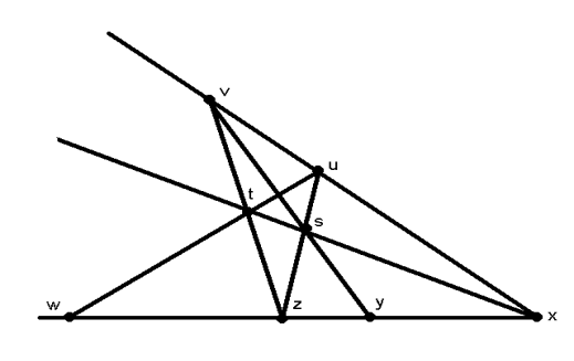
Figure 1: Harmonic conjugation

Soler’s axiom may be phrased as follows:

SO  If $x$ and $y$ are orthogonal atoms then there is $z\leq x\cup y$ such that $w=\mathcal{H}(z;x,y)$ is orthogonal to $z$. In other words, $\mathcal{H}(z;x,y)=z^{\bot}\cap(x\cup y)$.

Intuitively, such a $z$ bisects the angle between $x$ and $y$, that is, defines $\sqrt{2}$ in the field $K$. Soler’s proved

Theorem 1

If $L$ is infinite dimensional and satisfies SO then $K$ is $\mathbb{R}$ or $\mathbb{C}$ or the quaternions.

In fact she proved a stronger result, assuming only that there is an infinite sequence of orthogonal atoms $\{x_{i}\}_{i\in\mathbb{N}}$ such that $x=x_{i}$ and $y=x_{i+1}$ satisfy SO for every $i=1,2,..$. The axiom SO may be given a probabilistic interpretation in the spirit Ramsey as we shall see subsequently.

3 Probability Measures: Gleason’s theorem, Wondergraph and Solèr’s axiom.

3.1 Gleason’s theorem

Assume that the set of possible events (or possible measurement outcomes, or propositions) is the lattice $L=L(\mathbb{H)}$ of subspaces of a real or complex Hilbert space $\mathbb{H}$. For simplicity, we shall concentrate on the finite dimensional case. Our aim is to tie this structure to probabilities, and by doing so to provide further evidence that the elements of $L$ can be seen as representing quantum events. Moreover, we shall see how the traditional features and ”paradoxes” of quantum mechanics are expressed and resolved in the quantum probabilistic language.

First a few words to connect measurements and outcomes in the more traditional view with the present notations. Here we shall be concerned with measurements that have a finite set of possible outcomes. Let $A$ be an observable (a Hermitian operator) with $n$ distinct possible numerical real values (the eigenvalues of $A$) $\alpha_{1,}\alpha_{2,...,}\alpha_{n}$. With each value corresponds an event $x_{i}=\{A=\alpha_{i}\}$ meaning “the outcome of a measurement of $A\$is$\ \alpha_{i}$” We identify this event with the subspace of $\mathbb{H}$ spanned by the eigenvectors of $A$ having the eigenvalue $\alpha_{i}$. The events $x_{i}$ are pair-wise orthogonal elements of $L$. The sub lattice that $x_{1},x_{2},...,x_{n}$ generate is a finite Boolean algebra which we shall denote by $\mathcal{B}=\left\langle x_{1},x_{2},...,x_{n}\right\rangle$. In case $n$ is the dimension of the space $\mathbb{H}$ each one of the events $x_{i}$ is an atom and the observable $A$ is said to be maximal.

Subsequently we shall identify any observable $A$ with the Boolean algebra $\left\langle x_{1},x_{2},...,x_{n}\right\rangle$ generated by its outcomes. Note that this is an unusual identification. It means that we equate the observables $A$ and $f(A)$, whenever $f$ is a one-one function defined on the eigenvalues of $A$. This step is justified since we are interested in outcomes and not their labels, and hence in such a “scale free” concept of observable. (It is like replacing the numbers $1,2,...,6$ on the face of a die by the numbers $2,3,...,7$ respectively). The converse is also true, with each orthogonal set of elements $x_{1},x_{2},...,x_{n}$ of $L$ there corresponds an observable whose eigenspaces include these elements.

Probability measures which are definable on $L$ were characterized many years ago in case $n=\dim\mathbb{H\geq}3$. Since every set of $n$ orthogonal atoms represents the outcomes of a possible measurement, and since they are all the possible outcomes we are motivated to introduce

Definition 1

Suppose that $\mathbb{H}$ is of a finite dimension $n$ over the complex or real field. A real function $P$ defined on the atoms in $L$ is called a state (or alternatively, a probability function) on $\mathbb{H}$ if the following conditions hold

1. $P(0)=0$, and $P(y)\geq 0$ for every element $y\in L$.

2. If $x_{1},x_{2},...,x_{n}$ is an orthogonal set of atoms then $\sum_{j=1}^{n}P(x_{j})=1$.

The probability of every lattice element $y\in L$ is then fixed since it is a union of a set of orthogonal atoms $y=x_{1}\cup...\cup x_{r}$, so that $P(y)=\sum_{j=1}^{r}P(x_{j})$. A complete description of the possible states is given by Gleason’s theorem [29]:

Theorem 2

Given a state $P$ on a space of dimension $\geq 3$ there is an Hermitian, non negative operator $W$ on $H$, whose trace is unity, such that $P(x)=<\overset{\rightarrow}{x},W\overset{\rightarrow}{x}>$ for all atoms $x\in L$, where $<,>$ is the inner product, and $\overset{\rightarrow}{x}$ is a unit vector along $x$. In particular, if some $x_{0}\in L$ satisfies $P(x_{0})=1$ then $P(x)=\left|<\overset{\rightarrow}{x}_{0},\overset{\rightarrow}{x}>\right|^{2}$ for all $x\in L$ (Born’s rule).

With the obvious conditions on convergence the above definition and theorem generalize to the infinite dimensional case. The remarkable feature exposed by Gleason’s theorem is that the event structure dictates the quantum mechanical probability rule. It is one of the strongest pieces of evidence in support of the claim that the Hilbert space formalism is just a new kind of probability theory. The quantum structure is in this sense much more constrained than the classical formalism. The structure of the phase space of a classical system does not gratly restrict the type of probability measures that can be defined on it. The probability measures which are actually used in classical statistical mechanics are introduced mostly by fiat or, in any case, are very hard to justify.

Gödel [30] said in a different context : ”A probable decision about the truth [of a new axiom] is possible … inductively by studying its “success”. Success here means fruitfulness in consequences in particular “verifiable” consequences, i.e., consequences demonstrable without the axiom”. Importing this insight from the mathematical domain to the present physical domain we can see how the set of axioms for the structure, most of which are shared with classical probability, give rise to the quantum mechanical probabilistic structure which is otherwise left a mystery.

3.2 Finite gambles and uncertainty

So far we have dealt with the lattice $L$ in its entirety, and with everywhere defined probability functions. The standard conceptions of Bayesian probability theory make do, initially at least, of finite probability spaces. A canonical situation handled by this theory is that of a gamble. In the words of Ramsey: “The old-established way of measuring a person’s belief ” by proposing a bet, and seeing what are the lowest odds which he will accept, is “fundamentally sound” [4]. Our gambles will likewise be finite and consist of four steps

1. A single physical system is prepared by a method known to everybody.

2. A finite set $\mathcal{M}$ of incompatible measurements, each with a finite number of possible outcomes, is announced by the bookie. The agent is asked to place bets on the possible outcomes of each one of them.

3. One of the measurements in the set $\mathcal{M}$ is chosen by the bookie and the money placed on all other measurements is promptly returned to the agent.

4. The chosen measurement is performed and the agent gains or looses in accordance with his bet on that measurement.

There are two reasons to concentrate on finite gambles of this kind. First, to avoid over idealization; for it is hard to imagine someone betting on the outcomes of all possible measurements (perhaps writing an IOU for each one of them). Secondly, and more importantly, the infinite idealization blurs the important fact that indeterminacy, and all other ”strange” results associated with quantum theory, are fundamentally combinatorial. The non-classical behavior of the probabilities is already forced by a finite number of events and the relations among them.

Recall that each measurement is identified with the Boolean algebra generated by its possible outcomes in $L$: $\mathcal{B}=\left\langle x_{1},x_{2},...,x_{m}\right\rangle$  (the $x_{i}$’s may not be atomic in case $\mathcal{B}$ is not a maximal measurement). So a gamble $\mathcal{M}$ is just a set of such algebras $\mathcal{M=\{B}_{1},\mathcal{B}_{2},...,\mathcal{B}_{k}\}$. We do not assume that the gambler knows quantum theory. All she is aware of is the logical structure which consists of these sets of outcomes. In particular, she recognizes identities, and the cases where the same outcome is shared by more than one experiment. By acting according to the standards of rationality the gambler will assign probabilities to the outcomes. To see this, assume that $P(x\mid\mathcal{B})$ is the probability assigned by the agent to the outcome $x$ in measurement $\mathcal{B}$, where $\mathcal{B}\in\mathcal{M}$ and$\ x\in$ $\mathcal{B}$.

RULE 1: For each measurement $\mathcal{B}\in\mathcal{M}$ the function $\ P(\cdot\mid\mathcal{B})$ is a probability distribution on $\mathcal{B}$.

This follows directly from classical probability theory. Recall that after the third stage in the quantum gamble the agent faces a bet on the outcome of a single measurement. The situation at this stage is essentially the same as a tossing of a coin or a casting of a die. Hence, the probability values assigned to the possible outcomes of the chosen measurement should be coherent.

RULE 2: If $\mathcal{B}_{1},\mathcal{B}_{2}\in\mathcal{M}$,  and $y\in\mathcal{B}_{1}\cap\mathcal{B}_{2}$ then $P(y\mid\mathcal{B}_{1})=P(y\mid\mathcal{B}_{2})$.

The rule asserts the non contextuality of probability, discussed in section 2.1. Suppose that $\mathcal{B}_{1}=\left\langle x_{1},x_{2},...,x_{m}\right\rangle$ and $\mathcal{B}_{2}=\left\langle z_{1},z_{2},...,z_{r}\right\rangle$ then $y\in\mathcal{B}_{1}\cap\mathcal{B}_{2}$ implies that $(x_{1}\cap y)\cup...\cup(x_{m}\cap y)=y=(z_{1}\cap y)\cup...\cup(z_{r}\cap y)$. Rule 2, therefore, follows from this identity between events, and the principle that identical events in a probability space have equal probabilities.

To take the discussion closer to the lattice theoretic conception consider finite subsets of events, $\Gamma\subset L$.

Definition 2

Two propositions $x$ and $y$ of $\Gamma$ are compatible if $x=(x\cap y)\cup\nolinebreak(x\cap y^{\bot})$ and $y=(y\cap x)\cup(y\cap x^{\bot})$. A state (or probability function) $\Gamma$ is a real function $P$ on $\Gamma$ such that

a. $P(x)\geq 0$ for all $x\in\Gamma$

b. $P(x^{\bot})=1-P(x)$ whenever $x,x^{\bot}\in\Gamma$

c. $P(x\cup y)+P(x\cap y)=P(x)+P(y)$ whenever $x$ and $y$ are compatible and $x,y\in\Gamma$.

Such probability functions defined over finite subsets of events in the lattice are the subject of our study. Note that we do not put any requirements on such $P$’s apart from the three conditions a, b, c, in the definition. In particular, probability functions on $\Gamma$ are not constrained to be induced by quantum mechanical states. The relation between this definition and the gambles introduced previously is clear. Given any gamble $\mathcal{M}$ as above the set of events is $\Gamma=\mathcal{B}_{1}\cup\mathcal{B}_{2}\cup...\cup\mathcal{B}_{k}\subset L$. Every probability function which follows RULE 1 and RULE 2 satisfy the conditions a, b, c, in definition 2.

As a simple example which demonstrates an uncertainty relation consider the following quantum gamble $\mathcal{M}$ consisting of seven incompatible measurements (Boolean algebras), each generated by its three possible atomic outcomes:

$$\left\langle x_{1},x_{2},y_{2}\right\rangle,\ \left\langle x_{1},x_{3},y_{3}\right\rangle,\ \left\langle x_{2},x_{4},x_{6}\right\rangle,\ \left\langle x_{3},x_{5},x_{7}\right\rangle,\vskip 3.0pt plus 1.0pt minus 1.0pt$$

$$\ \left\langle x_{6},x_{7},y\right\rangle,\ \left\langle x_{4},x_{8},y_{4}\right\rangle,\ \left\langle x_{5},x_{8},y_{5}\right\rangle$$

Note that some of the outcomes are shared by two measurements, these are denoted by the letter $x$. The other outcomes each belong to a single algebra, and are denoted by a $y$. The orthogonality relations among the generators are depicted in the orthogonality graph in Fig(2), which is a part of Kochen and Specker’s famous ”cat’s cradle”[31]. Each node in the graph represents an outcome, two nodes are connected by an edge if, and only if the corresponding outcomes belong to a common Boolean algebra (measurement); each triangle represents the generators of one of the Boolean algebras.

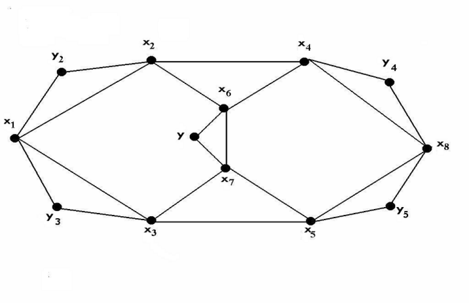
Figure 2: Cat’s cradle

The probabilities of each triple of outcomes of each measurement should sum to 1, for example, $P(x_{4})+P(x_{8})+P(y_{4})=1$. There are altogether seven equations of this kind. Combining them with the fact that probability is non-negative it is easy to prove that the probabilities assigned by our rational agent should satisfy $P(x_{1})+P(x_{8})\leq\frac{3}{2}$ [15]. This is an example of an uncertainty relation, a constraint on the probabilities assigned to the outcomes of incompatible measurements. In particular, if the system is prepared in such a way that it is rational to assign $P(x_{1})=1$ then the rules of quantum gambles force $P(x_{8})\leq\frac{1}{2}$.

This result is a special case of a more general principle given by [32, 33]

Theorem 3

(logical indeterminacy principle) Assuming $\dim\mathbb{H}\geq 3,$ let $x$ and $y$ be two incompatible atoms in the lattice $L=L(\mathbb{H)}$, that is, $x\neq(x\cap y)\cup(x\cap y^{\bot})$. Then there is a finite set $\Gamma\subset L\mathbb{(H})$ with $x,y\in\Gamma$ such that every state $P$ on $\Gamma$ satisfies $P(x)+P(y)<2$. In fact we have more: $P(x),P(y)$ $\in\{0,1\}$ if and only if $P(x)=P(y)=0$.

This theorem explains the sense in which axiom H4 -the axiom of irreducibility- expresses indeterminacy. This axiom asserts that for every non trivial $x$ there is a $y$ such that $x\neq(x\cap y)\cup(x\cap y^{\bot})$. By the logical indeterminacy principle the probability value of at least one of the events $x$ or $y$ must be strictly between zero and one, unless they both have probability zero. Moreover, this fact is already forced by the relation between $x$, $y$ and finitely many other events. Remember also that H4 is the only axiom (except SO) that distinguishes between the classical and quantum structures.

3.3 Wondergraph

The previous theorem is typical in the sense that all features of quantum probability, even the quantitative features, can be forced by the logical relations among finitely many events. This follows from a construction of a particular finite set of atoms in $\mathbb{R}^{3}$ which, together with the orthogonality relations among its elements will be called the Wondergraph.

Let us introduce first the notion of a frame function which generalizes the concept of a state

Definition 3

Let $\Gamma\subseteq L(\mathbb{H})$ be a set of atoms of $L(\mathbb{H})$ where $\dim\mathbb{H}=n$. A frame function on $\Gamma$ is a real function $f$ on $\Gamma$ such that all orthogonal sets of atoms $x_{1},x_{2},...,x_{n}$ in $\Gamma$ satisfy $\sum_{j=1}^{n}f(x_{j})=C$; where $C$ is a constant.

Consider the case of $\mathbb{R}^{3}$ the smallest space to which Gleason’s theorem applies. Let $\overrightarrow{e_{1}}=(1,0,0)$, $\overrightarrow{e_{2}}=(0,1,0)$ and $\overrightarrow{e_{3}}=(0,0,1)$ be the standard basis in $\mathbb{R}^{3}$ and $\overrightarrow{b_{ij}}=\frac{1}{\sqrt{2}}(\overrightarrow{e_{i}}+\overrightarrow{e_{j}})$, $1\leq i<j\leq 3$. Denote by $e_{i}$ and $b_{ij}$ the one dimensional subspaces along these vectors. The following theorem turns out to be equivalent to Gleason’s theorem [33]:

Theorem 4

(Wondergraph theorem) For every atom $z\in L(\mathbb{R}^{3})$ there is a finite set of atoms $\Omega(z)\subset L(\mathbb{R}^{3})$ such that $e_{i},b_{ij},z\in\Omega(z)$ and such that every frame function $f$ on $\Omega(z)$ which satisfies $f(e_{i})=f(b_{ij})=0$, and $\left|f(x)\right|\leq 1$ for all $x\in\Omega(z)$ necessarily also satisfies $\left|f(z)\right|\leq\frac{1}{2}$. Moreover, $\left|\Omega(z)\right|$, the number of elements of $\Omega(z)$, is  the same for all $z$.

Note that the condition $f(e_{i})=0,$ $\ 1\leq i\leq 3$ for the frame function $f$ on $\Omega(z)$ entails that $f(x)+f(x^{\prime})+f(x^{\prime\prime})=0$ for all orthogonal triples $x,x^{\prime},x^{\prime\prime}\in\Omega(z)$. To see why Wondergraph theorem entails Gleason’s theorem consider first

Lemma 5

Gleason’s theorem for $\mathbb{R}^{3}$is true if and only if every bounded frame function $f$ defined on the atoms of $L(\mathbb{R}^{3})$ which satisfies $f(e_{i})=f(b_{ij})=0$ is identically zero.

The proof of the lemma is straightforward. It follows from the fact that the quadric form $\left\langle\overrightarrow{x},A\overrightarrow{x}\right\rangle$ induced by a self adjoint operator $A$ on $\mathbb{R}^{3}$ is uniquely determined by the six  numbers $\left\langle\overrightarrow{e_{i}},A\overrightarrow{e_{i}}\right\rangle$, $\left\langle\overrightarrow{b_{ij}},A\overrightarrow{b_{ij}}\right\rangle$. Now, to see how Gleason’s theorem follows from Wondergraph let $f$ be a bounded frame function defined on the atoms of $L(\mathbb{R}^{3})$ which satisfies $f(e_{i})=f(b_{ij})=0$. Normalize $f$ so that $\left|f(x)\right|\leq 1$ for all $x$. Take $z$ to be arbitrary, then the restriction of $f$ to $\Omega(z)$ is a frame function on $\Omega(z)$ and therefore $\left|f(z)\right|\leq\frac{1}{2}$. Suppose the atoms of $\Omega(z)$ are $x_{1},...,x_{s}$ and consider the set $\Omega_{1}(z)=\bigcup_{j=1}^{s}\Omega(x_{j})$. The restriction of $f$ to $\Omega_{1}(z)$ is a frame function on each one of the $\Omega(x_{j})$’s. Hence, $\left|f(x_{j})\right|\leq\frac{1}{2}$ for all $x_{j}\in\Omega(z)$ and therefore $\left|f(z)\right|\leq\frac{1}{4}$. Iterating this process we get that $\left|f(z)\right|$ becomes as small as we wish. Since $z$ is arbitrary the theorem follows. Gleason’s theorem for any Hilbert space follows from the case of $\mathbb{R}^{3}$, as Gleason himself showed. Another way to extend the theorem from $\mathbb{R}^{3}$ to higher real or complex dimensions is to construct Wondergraphs in every (finite) dimension; which can be done once the three dimensional real case is given.

The proof that Gleason’s theorem entails the existence of Wondergraph is based on model theory. As a part of the proof one also concludes that there is a known algorithm to construct Wondergraph. The setback is that this algorithm runs very slowly (it is, in fact , the decision algorithm for the theory of real closed fields, which in the worst case runs in doubly exponential time). Thus we pose a

Problem 1

Construct Wondergraph explicitly.

Wondergraph allows one to reduce all the interesting quantum phenomena to relations among finitely many events. This follows from:

Corollary 6

Given a finite set of atomic events $\Gamma_{0}$ and a real number $\varepsilon>0$ there is a finite set of atoms $\Gamma$ such that

a. $\ \Gamma_{0}\subset\Gamma$, the number of elements $\left|\Gamma\right|$ of $\Gamma$ depends on $\varepsilon$ and on $\left|\Gamma_{0}\right|$ but not on the elements of $\Gamma_{0}$.

b.  If $P$ is a state on $\Gamma$ then there is a quantum state $W$ (non negative Hermitian operator with trace $1$) such that

$$\left|P(x)-<\overset{\rightarrow}{x},W\overset{\rightarrow}{x}>\right|<\varepsilon\quad for\ all\ x\in\Gamma_{0}$$

c. There is an algorithm to generate $\Gamma$ given $\Gamma_{0}$ and $\varepsilon$.

For many of the famous ”paradoxes” of quantum mechanics explicit constructions of the required finite set $\Gamma$ exist [15, 32, 33]. These include the EPR-Bell argument, the Kochen and Specker theorem, and also generalizations of Kochen and Specker to any given finite number of colors.

On a more fundamental level the importance of these results lies in the way probabilities are associated with $L$, the algebra of all the possible outcomes of all possible measurements. Remember that in the epistemic conception of probability a “fundamentally sound” method of measuring a person’s belief is “by proposing a bet and seeing what are the lowest odds he will accept”. In order to fit the infinite structure $L$ into this view of probability (or any other of the standard Bayesian accounts) we consider only finite segments of $L$ and the probability functions definable on them. These are the quantum gambles considered above. They are the equivalents of classical gambles with dice, roulettes and cards. Some real experiments involve arrangements which are like our gambles: A laboratory device is prepared in such a way that it can perform either one of a few incompatible measurements. Then, the experiment which is actually performed is chosen at random. This gives quantum probability an ”operational” flavour and, hopefully removes some of the mystery connected with it, typically expressed by words like ”interference” and ”superposition”.

Another way to see this point is to think about the classical propositional calculus. The Lindenbaum-Tarski algebra on countably many generators gives us all the expressive power we need as far as the propositional connectives are concerned. However, in practice we interpret (assign truth values) only to finite subsets. By analogy, if we take $L$ as representing a ”syntax” encompassing symbols for all possible outcomes of all possible measurements, then the ”semantics” is the assignment of probability values to finite sections of $L$. Gleason’s theorem, in its Wondergraph version, implies that this ”semantics” is, in fact, complete:

Corollary 7

(Completeness) Suppose that an agent assigns probability values $P(x)$ to the elements $x$ of a finite $\Gamma_{0}\subset L$, in a way that contradicts all possible quantum assignments. Then there is a finite $\Gamma\supset\Gamma_{0}$, such that $P$ cannot be extended from $\Gamma_{0}$ to $\Gamma$. Hence, in a larger gamble the agent can be shown to be irrational.

3.4 Solèr’s axiom revisited

Let us return to our axiomatic system and the axiom that closes the gap. Recall that Solèr’s axiom asserts that for every pair of orthogonal atoms $x$ and $y$ there is another atom $z$ in the plane they span, which bisects the angle between $x$ and $y$. More formally: $\mathcal{H}(z;x,y)$, the harmonic conjugate of $z$ with respect to $x$ and $y$, is orthogonal to $z$.

Assume that $L$ is infinite dimensional. In this case Solèr’s theorem, when coupled with Gleason’s theorem, implies that for any (globally defined) state $P$ on $L$ and atoms $x,y\in L$, if $P(x)=1$ and $P(y)=0$ then necessarily $x\bot y$, and there is an atom $z\leq x\cup y$ such that $P(z)=\frac{1}{2}$. In other words, there is a precise interpolation between probabilities zero and one.

The axiomatic systems of Bayesian probability theory typically include axioms which imply interpolation of probability values. The most famous (or infamous) one is Ramsey’s axiom on the existence of an ”ethically neutral” proposition whose probability is one half (axiom 1 in Ramsey’s system [4]). The axiom allows Ramsey to construct his theory of utilities (or ”values”, in his terminology). Savage [5], who wanted to avoid notions like ”ethical neutrality”, nevertheless also needs an interpolation principle for probabilities, and assumes the existence of arbitrarily refined partitions. This implies that one can obtain propositions with probabilities arbitrarily close to any rational in the interval $[0,1]$.

I propose to read Solèr’s axiom as a probability interpolation axiom; or at any rate to reformulate or replace it by a direct axiom about probabilities. This, however, cannot be straightforward. We are not even guaranteed that a globally defined state exists on $L$ in the first place. However, we can use the fact that certain finite orthogonality graphs such as $\Gamma$ of theorem 3 force any state defined on them to interpolate probability values between zero and one. This is our logical indeterminacy principle which expresses probabilistically the basic principle that differentiates the quantum event structure from the classical one. Now, we can turn the tables and assert axiomatically that orthogonality relations like those in $\Gamma$ are realizable in $L$. This assertion indirectly expresses the indeterminacy relations in their probabilistic sense. Here, for example, is how this can be done:

Consider $L(\mathbb{R}^{3})$ and the rays $x$, $z$ through the vectors:$\overrightarrow{x}=(1,0,0)$, and $\overrightarrow{z}=(1,1,0)$ respectively. Let $\Gamma=\Gamma(x,z)\subset L(\mathbb{R}^{3})$ be the finite subset of rays guaranteed in theorem 3 (and explicitly constructed in [31, 32]). This means that if $P$ is a state on $\Gamma$ with $P(x)=1$ then $0<P(z)<1$. Now, consider the rays in $\Gamma$ and their orthogonality relations abstractly, that is, as a graph, which we shall also denote $\Gamma$. A candidate to replace Solèr’s axiom can then be formulated as :

SO* Let $x$, $y$, $x^{\prime}\in L$ be three orthogonal atoms then there is $z\leq x\cup y$, such that the graph $\Gamma(x,z)$ is realizable in $x\cup y\cup x^{\prime}$.

There is a way to construct the graph $\Gamma$ which will make SO* obviously stronger than the original SO. To do this simply add to $\Gamma$ the rays (and orthogonality relations) which force the relation $\mathcal{H}(z;x,y)\ \bot\ z$. In the notations of section 2.4, this means adding rays $u,v,s,t$ and also the rays which, in the space $x\cup y\cup x^{\prime}$, are orthogonal to the planes $x\cup u$, $z\cup u$, $y\cup v$, $x\cup s$, $z\cup v$, $u\cup t$ . But this is cheating, all it shows is that there is a finite graph that forces Solèr’s axiom simultaneously with uncertainty. In order to make the axiom more acceptable one has to solve

Problem 2

Find the minimal $\Gamma$ that forces logical indeterminacy and that allows the proof of Solèr’s theorem (and even, perhaps, improves it to include finite dimensional cases).

Another possible candidate -analogous to Savage’s axiom on the existence of arbitrarily fine partitions- is the following:

SO** Let $z\in L$; then the Wondergraph $\Omega(z)$ is realizable in any three dimensional subspace of $L$ that includes $z$.

The restriction of the graphs we have used to those realizable in $\mathbb{R}^{3}$ is not essential. It may very well be that a more natural candidate for our $\Gamma$ or $\Omega$ exists, e.g., in $\mathbb{C}^{4}$.

4 Probability: Range and Classical Limit

We turn now to the explanatory power of our analysis. The ”logic of partial belief” provides straightforward probabilistic, or even combinatorial derivations of a variety of phenomena for which alternative approaches require complicated ad-hoc dynamical explanations. We shall consider two central examples: the first is the EPR paradox and the violation of Bell inequality, and the second is the measurement problem. In particular, we shall discuss the way macroscopic objects can be handled in this framework.

4.1 Bell Inequalities

The phenomenological difference between classical and quantum probability is most dramatic when quantum correlations associated with entangled states are concerned. Let us recall what the classical probabilistic analysis of the situation is: A pair of objects is sent from the source, one in Alice’s direction, one in Bob’s direction. Alice can perform either one of two measurements on her object; she can decide to detect the event $x_{1}$ or its absence (which means detecting the event $x_{1}^{\bot}$). Alternatively, she can decide to check the event $x_{2}$ or $x_{2}^{\bot}$. So each of these measurements has two possible outcomes. Similarly, Bob can test for $y_{1}$ or use a different test to detect $y_{2}$. Assuming nothing about the physics of the situation, and just considering the outcomes we get the following possible logical combinations expressed in the truth table:

$$\begin{array}[c]{cccccccc}x_{1}&x_{2}&y_{1}&y_{2}&x_{1}\cap y_{1}&x_{1}\cap y_{2}&x_{2}\cap y_{1}&x_{2}\cap y_{2}\\ 0&0&0&0&0&0&0&0\\ ...&...&...&...&...&...&...&...\\ 1&1&0&1&0&1&0&1\\ ...&...&...&...&...&...&...&...\\ 1&1&1&1&1&1&1&1\end{array}$$

It is the truth table of four propositional variables $x_{1},x_{2},y_{1},y_{2}$ and four (out of the six) pair conjunctions, so it has $16$ rows, three of them shown explicitly. Each row represents a possible state of affairs regarding the possible outcomes where $1$ indicates that the event occurs. Now, suppose that we were to bet on the outcomes. There are, of course many ways to do this, but they all have to conform with the canons of rationality. The only constraint here is that each one of the $16$ possibilities will be assigned a non-negative probability, and the sum of these probabilities be $1$. To give this fact a geometric interpretation consider each one of the $16$ rows in the truth table as a vector in an $8$ dimensional real space, then the vector of probabilities (writing $x_{i}y_{j}$ for $x_{i}\cap y_{j}$)

$$\mathbf{P}=(P(x_{1}),P(x_{2}),P(y_{1}),P(y_{2}),P(x_{1}y_{1}),P(x_{1}y_{2}),P(x_{2}y_{1}),P(x_{2}y_{2}))$$

lies in the convex hull of these $16$ vectors, which is a correlation polytope in $\mathbb{R}^{8}$ with the $16$ truth values as vertices shown schematically in Fig(3).

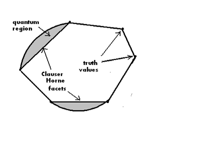
Figure 3: Classical and quantum correlations

The facets of the polytope, are given by linear inequalities in the probabilities, in this case the non-trivial inequalities have the form

$$-1\leq P(x_{1}y_{1})+P(x_{1}y_{2})+P(x_{2}y_{2})-P(x_{2}y_{1})-P(x_{1})-P(y_{2})\leq 0$$ (4)

They are called Clauser-Horne inequalities, they are among what is generally known as Bell inequalities. Remarkably, in the mid 19-century George Boole considered the most general form of the constraints on the values of probabilities of events that can be derived from the logical relations among them. He proved that these constraints have the form of linear inequalities in the probabilities. Paraphrasing Kant he called such constraints Conditions of Possible Experience.

So far we have been concentrating on the classical picture. What is the quantum mechanical analysis? Again, we shall make no physical assumptions beyond those which are given by the axioms of the event structure. With the two particles we associate a Hilbert space of the form $H\otimes H$, where in case the objects are spin-${\frac{1}{2}}$ particles, $\dim H=2$. The relevant lattice is thus $L=L(H\otimes H)$. The element of $L$ corresponding to the event $x_{1}$ is a two dimensional subspace of the form $a_{1}\otimes 1$ where $a_{1}\in L(H)$ and $1$ is the unit in $L(H)$. Similarly, the event corresponding to the outcome $y_{1}$ on Bob’s side is $1\otimes b_{1}$, and likewise for the other cases. The event corresponding to the measurement of $x_{1}$ on Alice’s side and $y_{1}$ on Bob’s side is just the intersection:

$$(a_{1}\otimes 1)\cap(1\otimes b_{1})=a_{1}\otimes b_{1}$$

Note also that $a_{i}\otimes 1$, and $1\otimes b_{j}$ are compatible. Now, to the eight outcomes

$$\begin{array}[c]{cccccccc}a_{1}\otimes 1,&a_{2}\otimes 1,&1\otimes b_{1},&1\otimes b_{2},&a_{1}\otimes b_{1},&a_{1}\otimes b_{2},&a_{2}\otimes b_{1},&a_{2}\otimes b_{2},\end{array}$$

correspond an $8$ dimensional vectors of probability values

$$\mathbf{P}=(P(a_{1}\otimes 1),P(a_{2}\otimes 1),P(1\otimes b_{1}),P(1\otimes b_{2}),P(a_{1}\otimes b_{1}),P(a_{1}\otimes b_{2}),P(a_{2}\otimes b_{1}),P(a_{2}\otimes b_{2})),$$

where $P$ is any probability assignment to the elements of $L(H\otimes H)$. When we vary $P$ and the subspaces $a_{i}$, $b_{j}$, we see that the quantum range is larger than the classical one, and some points lie outside the classical polytope (Fig 3), that is, they violate one of the facet inequalities of Clauser and Horne.

From the point of view developed so far this consequence is natural and follows from the event structure of quantum mechanics via Gleason’s theorem. We also know from corollary 10 that a violation of a Clauser-Horne inequality can already be depicted in a finite gamble (an explicit construction can be found in [15]). Altogether, in our approach there is no problem with locality and the analysis remains intact no matter what the kinematic or the dynamic situation is; the violation of the inequality is a purely probabilistic effect. Notice that we are just using the quantum event space notion of intersection between (compatible) outcomes: $(a_{1}\otimes 1)\cap(1\otimes b_{1})=a_{1}\otimes b_{1}$, as we have used the intersection in the classical event space. The derivation of Clauser-Horne inequalities, indeed of many of Boole’s conditions, is blocked since it is based on the Boolean view of probabilities as weighted averages of truth values. This, in turn, involves the metaphysical assumption that there is, simultaneously, a matter of fact concerning the truth values of incompatible propositions such as $x_{1}=a_{1}\otimes 1$ and $x_{2}=a_{2}\otimes 1$.

Recall that in section 2.2 we restricted ”matters of fact” to include only observable records. Our notion of “fact” is analytically related to that of “event” in the sense that a bet can be placed on $x_{1}$ only if its occurrence, or failure to occur, can be unambiguously recorded. However, this leaves open a metaphysical question: Given that $x_{1}$ occurred, what is the status of $x_{2}$ for which no observable record can exist? Our axioms are not designed to rule out the possibility that $x_{2}$ has a truth value which we do not know. Initially our approach was agnostic with respect to facts which leave no trace. However, as the above analysis shows, assigning truth values to $x_{2}$ and $x_{1}$ simultaneously is untenable. In other words, it is prohibited by the axioms a posteriori. I believe that Bohr deserves the credit for this insight, although his arguments fall short of establishing it.

We should also recall that there are alternatives to quantum mechanics in which the violations of the Clauser-Horne inequalities have non-local dynamical origins. However, from our perspective the commotion about locality can only come from one who sincerely believes that Boole’s conditions are really conditions of possible experience. Since these conditions are just properties of the classical intersection of events, their violation must indicate that something is not kosher with the measurements, that is, the choice of a measurement on one side may be correlated with the outcome on the other. But if one accepts that one is simply dealing with a different notion of probability, then all space-time considerations become irrelevant.

4.2 The BIG measurement problem, the small one, and the classical limit.

There are two “measurement problems” The BIG problem, which is illusory, and the small problem which is real and concerns the quantum mechanics of macroscopic systems. The BIG problem concerns those who believe that the quantum state is a real physical state which obeys Schrödinger’s equation in all circumstances. In this picture a physical state in which my desk is in a superposition of being in Chicago and in Jerusalem is a real possibility; and similarly a superposed alive-dead cat. In fact the linearity of Schrödinger’s equation implies that (decoherence notwithstanding) it is easy to produce states of macroscopic objects in superposition- which seems to contradict our experience, and sometimes, as in the cat case, does not even make much sense.

In our scheme quantum states are just assignments of probabilities to possible events, that is, possible measurement outcomes. This means that the updating of the probabilities during a measurement follows the Von Neumann-Lüders projection postulate and not Schrödinger’s dynamics. Indeed, the projection postulate is just the formula for conditional probability that follows from Gleason’s theorem. So the BIG measurement problem does not arise. In particular, the cat in the Schrödinger thought experiment is not superposed, but is rather cast in the unlikely role of a particle spin detector. Schrödinger’s equation governs the dynamics between measurements; it dictates the way probability assignments should change over time in the absence of a measurement. The general shape of the Schrödinger’s equation is not a mystery either; the unitarity of the dynamics follows from the structure of $L(\mathbb{H})$ via a theorem of Wigner [39], in its lattice theoretic form [40]. However, these remarks do not completely eliminate the measurement problem because in our scheme quantum mechanics is also applicable to macroscopic objects.

So suppose that $x$ is one of the rays in the cat’s Hilbert space corresponding to a living cat. Let $y$ be one of the atoms corresponding to a dead cat so that $x\bot y$. By Solèr’s axiom there is an atom $z\leq x\cup y$ which bisects the angle between $x$ and $y$. Does this mean that we are back with the BIG measurement problem? The answer is ‘No’; remember that $z$ is not a state of the system, it is a possible measurement outcome. It is a mistake to think that by merely following Schrödinger’s experiment we are ”observing” the event $z$, or something like it. Obviously we are not, we either see an $x$-like event, a live cat, or a $y$-like dead cat event. In order to ”see” $z$ we have to devise and perform a measurement such that $z$ is one of its eigenspaces. For reasons that will be explained below, with all probability this is impossible.

But even agreeing that performing such a measurement is impossible, we can surely think about operators for which $z$ is an eigenspace, say the projection on $z$. So let us imagine what one will see when one performs this measurement; what does the event $z$ look like? Presumably, the imagined measuring device is a huge piece of very complicated equipment, because in all likelihood the measurement of the projection on $z$ involves manipulating individual cat particles. In the end, however, there is a dial with two possible readings $0$ and $1$, and $z$ is just the event that the dial reads $1$. By Lüders’ rule the state of the cat after the measurement -assuming that $z$ was the outcome- is the projection on $z$. The quantum state is not a physical object, it is a representation of our state of knowledge, or belief. The projection on $z$ represents an extremely complex assignment of probabilities to all possible events in a Hilbert space of $\backsim 10^{25}$ particles, an intractable business. One thing is clear, though, there is complete uncertainty about the cat being dead or alive $P(x)=P(y)=\frac{1}{2}$, and of course $P(x\cup y)=1$.

Ignorance aside, is it not the case that now, after the measurement, there is a matter of fact about the cat being dead or alive? Well, No! As in all such circumstances we cannot say that there is a fact regarding this matter. It is impossible in principle to obtain a record concerning the cat being alive or dead simultaneously with the $z$-measurement. There is no fundamental difference between the present case and EPR, meaning that we cannot consistently maintain that the proposition “the cat is alive” has a truth value. But the devil is in the details; there is no way to tell from our completely schematic description what is going on in the laboratory. Consequently, there is no way to tell what is the biological state of the cat. It is only after we have mastered the details of the measuring process that we can understand the exact sense in which no record of $x$ or of $y$ is obtainable.

4.3 The Weak Entanglement Conjecture

The small measurement problem is the question why we do not routinely observe events like $z$ for macroscopic objects. More precisely why is it hard to observe macroscopic entanglement, and what are the conditions in which it might be possible? One answer which is certainly valid is decoherence- meaning that it is extremely hard to isolate large pieces of matter and equipment from environmental noise. Decoherence is a dynamical process and its exact character depends on the physics of the situation. I would like to point a possible more fundamental, purely combinatorial reason which is an outcome of the probabilistic structure: The entanglement of an average ray in a multiparticle Hilbert space is very weak. To make this intuition precise we have to quantify entanglement, and define what we mean by “average ray”.

To make the discussion simpler we shall concentrate on qbits. So our Hilbert space is composed of $n$ copies of the two dimensional complex Hilbert space $\mathbb{H}_{n}\mathbb{=C}^{2}\otimes\mathbb{C}^{2}\otimes...\otimes\mathbb{C}^{2}$, and $\dim\mathbb{H}_{n}=2^{n}$. An atom $s\in L(\mathbb{H}_{n}\mathbb{)}$ is called separable if it has the form $s=x_{1}\otimes x_{2}\otimes...\otimes x_{n}$ with $x_{i}\in L(\mathbb{C}^{2})$, otherwise an atom is called entangled. Also, we shall call the projections on separable (entangled) rays, separable (entangled, respectively) pure states. We keep the letter $s$ to designate separable atoms, and denote by $S\subset L(\mathbb{H}_{n}\mathbb{)}$ the set of all separable atoms. As usual if $x\in L(\mathbb{H}_{n}\mathbb{)}$ is a ray (atom), we shall denote by $\overrightarrow{x}$ a unit vector along it.

Now, suppose that we want to observe an entangled atom $x$. More precisely, we want to obtain a positive proof that it is indeed entangled. To do this we have to design a measurement that will distinguish the ray $x$ from all the separable atoms $s\in S$. A Hermitian operator that does this always exists, and will be called an entanglement witness for $x$, or in short, a witness. The normalization of witnesses is a matter of convention and for our purpose we shall use the following:

Definition 4

An Hermitian operator $W$ on $\mathbb{H}_{n}\mathbb{=C}^{2}\otimes\mathbb{C}^{2}\otimes...\otimes\mathbb{C}^{2}$ ($n$ copies) is called an entanglement witness if it satisfies

$$\sup\{\left|\left\langle\overrightarrow{s},W\overrightarrow{s}\right\rangle\right|\ ;\ s\in\nolinebreak S\}=\nolinebreak 1$$

while

$$\left\|W\right\|=\sup\{\left|\left\langle\overrightarrow{x},W\overrightarrow{x}\right\rangle\right|\ ;\ x\in L(\mathbb{H}_{n}\mathbb{)\}}>1.$$

So a witness is an observable whose expectation on every separable state is bounded between $-1$ and $1$, while it has an eigenvalue that is larger than $1$ in absolute value. Any one-dimensional eigenspace $x$ corresponding to this eigenvalue is obviously entangled. Denote by $\mathcal{W}_{n}$ the set of all entanglement witnesses on $\mathbb{H}_{n}$. One way to estimate how much a given $x\in L(\mathbb{H}_{n}\mathbb{)}$ is entangled is to calculate

$$\mathcal{E}(x)=\sup\{\left|\left\langle\overrightarrow{x},W\overrightarrow{x}\right\rangle\right|\ ;\ W\in\mathcal{W}_{n}\mathcal{\}}$$ (5)

A witness $W$ at which the value $\mathcal{E}(x)$ obtains is the best witness for the entanglement of $x$. If we allow that every measurement involves errors then the larger $\mathcal{E}(x)$ is, the more likely we are to actually observe it. The good news is that there are rays $x\in L(\mathbb{H}_{n})$ such that $\mathcal{E}(x)=\sqrt{2^{n}}$. These correspond to the the maximally entangled states, the so-called generalized GHZ states. However, it seems that such rays become more and more rare as $n$ increases. To formulate this intuition precisely, let $\mu_{n}$ be the normalized uniform (Lebesgue) measure on the unit sphere of $\mathbb{H}_{n}$. Then we

Conjecture 1

There is a universal constant $C>0$ such that

$$\mu_{n}\left\{\overrightarrow{x}\ ;\ \mathcal{E}(x)>C\sqrt{n\log n}\right\}\rightarrow 0\quad as\ n\rightarrow\infty$$ (6)

A similar result has been established for a large family of witnesses that for each $n$ contains $2^{2^{n}}$ witnesses, and which include those that give the best estimation for the GHZ states [44]; hence the conjecture.

I think the conjecture, if true, concerns our ability to observe macroscopic entanglement. There are two types of macroscopic or mesoscopic rays whose entanglement might be witnessed, and the conjecture concerns the second case:

1. There may be relatively rare cases in which the entanglement witness happens to be a thermodynamic observable, that is, an observable whose measurement does not require manipulation of individual particles but only the observation of some global property of the system. There are some indications that this may be the case for some spin chains and lattices [45].

2. Cases of very strong entanglement, like GHZ, which do require many manipulations of individual particles to be observed; however, the value of $\mathcal{E}(x)$ is large enough to give significant results that rise above the measurement errors. If we assume that the measurement errors are independent, then the total expected error grows exponentially with the number of particles that are manipulated. So, in general, one expects that only $x$’s for which $\mathcal{E}(x)$ is exponential in the number of manipulated particles could yield a significant outcome. The conjecture proposes that the proportion of such $x$ ’s is low.

To sum up: the answer to the question ”why don’t I see chairs in superposition” is twofold, decoherence surely, but even if we could turn it off, there is the combinatorial possibility that ”seeing” something like this is nearly impossible. All this, luckily, does not prevent the existence of exotic macroscopic superpositions that can be recorded.

5 Measurements

In this paper, all we have discussed is the Hilbert space formalism. I have argued that it is a new kind of probability theory that is quite devoid of physical content, save perhaps the indeterminacy principle which is built into axiom H4. Within this formal context there is no explication of what a measurement is, only the identification of ”observables” as Hermitian operators. In this respect the Hilbert space formalism is really just a syntax which represents the set of all possible outcomes, of all possible measurements. It is analogous to the mathematical concept of a probability space, in which certain subsets are identified as events. However, the mathematical theory of probability itself does not tell us the nature of the connection between these formal creatures and real events in the world.

But even before a connection is made between the formal and physical sense of measurement I think there is an interesting philosophical problem here. Our formalism seems to be consistent: there is a possible world where measurements and their outcomes behave in the way described above. This would not have been a serious problem if the classical theory of probability were not conceived as a priori in some sense. But the theory of probability is a part of what we take as our theory of inference, hence the term ‘logic of partial belief’. As such it is also a ground for the formation of rational expectations. Therefore, the fact that there is a consistent alternative poses a problem similar to the problem that non-Euclidean geometry raised even before general relativity. What should we make of a world in which Boole’s conditions of possible experience are violated for no reason other than the structure of probabilities described here?

What is real in the quantum world? Firstly, there are objects- particles about which the theory speaks- which are identified by a set of parameters that involve no uncertainty, and can be recorded in all circumstances and thus persist through time and context [46]. Among them are the rest mass, electric charge, baryonic number, etc. The other part of quantum reality consists of events, that is, recordings of measurements in a very broad sense of the word. Now, one has to distinguish between measurements on the one hand and interactions between material objects on the other. The latter are best described in the Heisenberg picture: There is a time dependent interaction Hamiltonian $H(t)$ which, like any other observable, defines at every moment $t$ a set of possible outcomes, one of the outcomes would obtain if $H(t)$ were measured. If, in addition, we have formed a belief about the state of the system at time $t=0$ (as a result of a previous measurement, say) we automatically have a probability distribution over the set of all possible outcomes of all possible measurements at each $t$. So each interaction constrains the set of possible outcomes in a certain specific way, and the question which interactions can actually be executed is an empirical question, to be tested by observing the outcomes and their distributions. Measurements are not interactions in this sense; although in the broad description of an experiment there is usually an interaction leading to the measurement.

It is impossible to give a precise definition of all the physical processes that deserve the name measurement; just as it is not possible to define the term event to which the theory of probability can be applied. Even a non-contextual definition of a singular concrete measurement is hard to provide; in this sense measurement outcomes are events ”under a description”, as philosophers say. Broadly speaking, a measurement is a process in which a material system $M$, prepared in a specific way, records some aspect of another system $S$, a recording that effects a permanent change in $M$, or at least one that lasts long enough. The outcomes to which we have referred throughout the paper are such recordings. Probably the best way to describe measurements is in informational terms. The information recorded by a measurement is systematic in the sense that a repeated conjunction of $M$ and $S$ yields the same set of results, and the frequency distribution over the set of results stabilizes in the long run. Of the same importance is the information that is lost during a measurement, the outcome that we could have obtained if any other measurement $M^{\prime}$ were performed instead of $M$ [47].

This description is broad enough to include the change that photons imprint on the receptors of the retina; it also includes the change caused by a proton hitting a rock on the dark side of the moon. There is nothing specifically human about measurements, nor does $M$ have to be associated with a macroscopic system. What constitutes a ”measuring device” cannot be determined beyond this broad description. However, there is a structure to the set of events. Not only does each and every type of measurement yield a systematic outcome; but also the set of all possible outcomes of all measurements -including those that have been realized by an actual recording- hang together tightly in the structure of $L(\mathbb{H})$. This is the quantum mechanical structure of reality.

Acknowledgements: This paper is the outcome of a three lecture series that I gave at the Patrick Suppes Center for the Interdisciplinary Study of Science and Technology, Stanford University. I would like to thank Patrick Suppes, Michael Friedman and Thomas Ryckman for their generous hospitality and the lively discussions. I also want to thank William Demopoulos and Ehud Hrushovski for many conversations on questions of philosophy, logic, and mathematics, and Jeremy Butterfield for his comments and suggstions. The research leading to this paper is supported by the Israel Science Foundation grant number 879/02.

References

- [1] Ghirardi, G.C., Rimini, A., and Weber, T. Unified dynamics for microscopic and macroscopic systems. Physical Review D 34, 470 (1984).
- [2] Bohm, D. and Hiley, B.J. The Undivided Universe: An ontological interpretation of quantum theory. London: Routledge, 1993.
- [3] Bell, J. S. Speakable and Unspeakable in Quantum Mechanics Cambridge: Cambridge University Press,
- [4] Ramsey, F.P. Truth and Probability. (1926) reprinted In D. H. Mellor (ed) F. P. Ramsey: Philosophical Papers. Cambridge: Cambridge University Press 1990
- [5] Savage, L.J. The Foundations of Statistics. London: John Wiley and Sons, 1954.
- [6] Feynman, R. P. The concept of probability in quantum mechanics. Second Berkeley Symposium on Mathematical Statistics and Probability, 1950, Berkeley: University of California Press, 553 (1951).
- [7] Feynman, R. P. and Hibbs, A. R. Quantum Mechanics and Path Integrals New York: McGraw-Hill, 1965.
- [8] Pitowsky , I. George Boole’s “conditions of possible experience” and the quantum puzzle. British Journal for the Philosophy of Science 45, 95-125 (1994).
- [9] Weinberg, S. Gravitation and cosmology: Principles and applications of the general theory of relativity, New York: John Wiley & Sons, 1972.
- [10] Pitowsky, I. Unified field theory and the conventionality of geometry. Philosophy of Science 51, 685-689 (1984).
- [11] Ben Menahem Conventionalism, Cambridge: Cambridge University Press (2005).
- [12] Bub, J. The Interpretation of Quantum Mechanics. Dordrecht: Reidel (1974).
- [13] Bub, J. Quantum Mechanics is About Quantum Information, Foundations of Physics 35, 541 (2005)
- [14] Barnum, H. Caves, C. M. Finkelstein, J. Fuchs, C. A. and Schack, R. Quantum probability from decision theory? Proceedings of the Royal Society of London A 456, 1175 (2000)
- [15] Pitowsky, I. Betting on the outcomes of measurements: A Bayesian theory of quantum probability Studies in the History and Philosophy of Modern Physics 34, 395 (2003).
- [16] Stairs, A. Kipske, Tupman and quantum logic: the quantum logician’s conundrum. This volume
- [17] Deutsch, D. Quantum theory of probability and decisions, Proceedings of the Royal Society of London A455, 3129 (1999);
- [18] Wallace, D. Everettian Rationality: defending Deutsch’s approach to probability in the Everett interpretation. Studies in the History and Philosophy of Modern Physics 34 415 (2003).
- [19] Birkhoff, G. and von Neumann, J. The logic of quantum mechanics. Annals of Mathematics 37, 823 (1936).
- [20] Finkelstein, D. Logic of quantum physics. Transactions of the New York Academy of Science 25, 621 (1963)
- [21] Putnam. H., The logic of quantum mechanics. (1968) reprinted in Mathematics Matter and Method - Philosophical Papers Volume1. Cambridge: Cambridge University Press, 1975.
- [22] Pitowsky, I. Quantum Probability, Quantum Logic, Lecture Notes in Physics 321, Heidelberg: Springer, 1989
- [23] Rédei, M. Why John von Neumann did not like the Hilbert space formalism of quantum mechanics (and what he liked instead). Studies in the History and Philosophy of Modern Physics 27, 493 (1996).
- [24] Solovay, R. M. A model of set-theory in which every set of reals is Lebesgue measurable. Annals of Mathematics 92, 1 (1970).
- [25] Young, W. J. Projective Geometry Chicago: Open Court 1930.
- [26] Artin, E. Geometric Algebra New York: John Wiley & Sons 1957.
- [27] Solèr, M. P. Characterization of Hilbert spaces with orthomodular spaces Communications in Algebra 23, 219 (1995).
- [28] Holland, S. S. Orthomodularity in infinite dimensions; a theorem of M. Solèr. Bulletin of the American Mathematical Society 32, 205 (1995).
- [29] Gleason, A. M. Measures on the closed subspaces of a Hilbert space. Journal of Mathematics and Mechanics 6, 885-893 (1957).
- [30] Gödel, K. What is Cantor’s continuum problem? in Feferman, S. (ed.) Kurt Gödel’s collected Papers, Vol II Oxford: Oxford University Press, 1990.
- [31] Kochen, S. and Specker, E. P. The problem of hidden variables in muantum Mechanics. Journal of Mathematics and Mechanics 17, 59-87 (1967).
- [32] Pitowsky, I. Infinite and finite Gleason’s theorems and the logic of indeterminacy. Journal of Mathematical Physics 39, 218 (1998).
- [33] Hrushovski, E. and Pitowsky, I. Generalizations of Kochen and Specker’s Theorem and the Effectiveness of Gleason’s Theorem. Studies in the History and Philosophy of Modern Physics 35, 177 (2004).
- [34] Clauser, J.F., Horne, M. A., Shimony, A., and Holt, R. A. Proposed experiment to test local hidden-variable theories. Physical Review Letters 23, 880 (1969).
- [35] Fine, A. Hidden variables, joint probability and Bell inequalities. Physical Review Letters 48, 291 (1982).
- [36] Pitowsky, I. and Svozil, K. New Optimal tests of quantum nonlocality. Physical Review A 64, 4102 (2001)
- [37] Boole, G. On the theory of probabilities. Philosophical Transactions of the Royal Society of London 152, 225 (1862).
- [38] Boole, G. The laws of Thought New York: Dover, 1958 (first published in 1854).
- [39] Wigner, E. P. Group Theory and its Applications to Quantum Mechanics of Atomic Spectra. New York: Academic Press (1959)
- [40] Uhlhorn, U. Representation of symmetry transformations in quantum mechanics. Arkiv Fysik 23, 307 (1963).
- [41] Mermin, N. D. Extreme quantum entanglement in a superposition of macroscopically distinct states Physical Review Letters. 65, 1838 (1990).
- [42] Werner, R. F. and Wolf, M. All multipartite Bell correlation inequalities for two dichotomic observables per site. Physical Review A 64, 032112 (2001)
- [43] Zukowski M. and Brukner C. Bell’s theorem for general N-qubit states. Physical Review. Letters 88 210401 (2002).
- [44] Pitowsky, I. Macroscopic objects in quantum mechanics-A combinatorial approach. Physical Review A 70 022103 (2004).
- [45] Brukner, C. and Vedral, V. Macroscopic thermodynamical witnesses of quantum entanglement quant-ph/0406040 (2004).
- [46] Ben Menahem, Y. Realism and quantum mechanics in A. van der Merve (ed): Microphysical Reality and Quantum Formalism Dordrecht: Kluwer, 1988.
- [47] Demopoulos, W. Elementary propositions and essentially incomplete knowledge: A framework for the interpretation of quantum mechanics Noûs 38, 86 (2004)