Exponential Operators, Dobiński Relations and Summability

P. Blasiak1,2, A. Gawron1, A. Horzela1, K. A. Penson2
and A. I. Solomon 2,3
1 H.Niewodniczański Institute of Nuclear Physics, Polish Academy of Sciences,
ul. Eliasza-Radzikowskiego 152, PL 31342 Kraków, Poland
2Laboratoire de Physique Théorique de la Matière Condensée, Université P. et M. Curie, Tour 24 - 2e ét., 4 Pl.Jussieu, F 75252 Paris Cedex 05, France 3Physics and Astronomy Department, The Open University,
Milton Keynes MK7 6AA, United Kingdom
pawel.blasiak@ifj.edu.pl,agnieszka.gawron@ifj.edu.pl,
andrzej.horzela@ifj.edu.pl, penson@lptl.jussieu.fr,
a.i.solomon@open.ac.uk
Abstract

We investigate properties of exponential operators preserving the particle number using combinatorial methods developed in order to solve the boson normal ordering problem. In particular, we apply generalized Dobiński relations and methods of multivariate Bell polynomials which enable us to understand the meaning of perturbation-like expansions of exponential operators. Such expansions, obtained as formal power series, are everywhere divergent but the Padé summation method is shown to give results which very well agree with exact solutions got for simplified quantum models of the one mode bosonic systems.

pacs:
03.65.Fd, 02.10.Ox, 02.30.Lt

Consider exponential operators of the form $\exp{(-\lambda{\cal H}_{\boldmath{\alpha}}({\hat{n}}))}$, where ${\cal H}_{\boldmath{\alpha}}({\hat{n}})=\sum_{i=1}^{N}\alpha_{i}{\hat{n}}^{i}$ is a polynomial of the number operator ${\hat{n}}$ (assumed to be bounded from below), $\alpha_{i}$’s play roles of coupling constants and $\lambda$ is an overall positive parameter. Calculation of the number state representation of $\exp{(-\lambda{\cal H}_{\boldmath{\alpha}}({\hat{n}}))}$ is straightforward

$$\langle l|\exp{(-\lambda{\cal H}_{\boldmath{\alpha}}({\hat{n}}))}|m\rangle=\exp{(-\lambda\sum_{i=1}^{N}\alpha_{i}{m}^{i})}\delta_{lm},$$ (1)

as well as its (standard) coherent state representation ($|z\rangle=\exp{(-\frac{|z|^{2}}{2})}\sum_{n=0}^{\infty}\frac{z^{n}}{\sqrt{n!}}|n\rangle$, ${\hat{n}}|n\rangle=n|n\rangle$, $\langle n|n^{\prime}\rangle=\delta_{nn^{\prime}}$, $a|z\rangle=z|z\rangle$ and $\langle z^{\prime}|z\rangle=\exp{\left(-\frac{1}{2}\left(|z^{\prime}|^{2}+|z|^{2}-2z^{\prime}z\right)\right)}$)

$$\langle z^{\prime}|\exp{(-\lambda{\cal H}_{\boldmath{\alpha}}({\hat{n}}))}|z\rangle=\langle z^{\prime}|z\rangle e^{-z^{\prime}z}\sum\limits_{k=0}^{\infty}\frac{\displaystyle(z^{\prime}z)^{k}}{\displaystyle k!}\exp{\left(-\lambda\sum_{i=1}^{N}\alpha_{i}{k}^{i}\right)}.$$ (2)

For the simplest example of ${\cal H}_{\boldmath{\alpha}}({\hat{n}})={\hat{n}}$ the r.h.s of Eqn.(2) is given in terms of the elementary function

$$\begin{array}[]{rcl}\langle z^{\prime}|\exp{(-\lambda{\hat{n}})}|z\rangle&=&\langle z^{\prime}|z\rangle e^{-z^{\prime}z}\sum\limits_{k=0}^{\infty}\frac{\displaystyle(z^{\prime}z)^{k}}{\displaystyle k!}\exp{(-\lambda k)}\\ &=&\langle z^{\prime}|z\rangle\exp{\left(z^{\prime}z\left(e^{-\lambda}-1\right)\right)}\end{array}$$ (3)

in which one recognizes the exponential generating function of the (exponential) Bell polynomials [1]

$$\exp{\left(x\left(e^{\lambda}-1\right)\right)}=\sum\limits_{k=0}^{\infty}\frac{\displaystyle\lambda^{k}}{\displaystyle k!}B(k,x).$$ (4)

The Bell polynomials are well known from their applications in combinatorics [2]. They are defined as

$$B(n,x)=\sum\limits_{k=1}^{n}S(n,k)x^{k},$$ (5)

where $S(n,k)$ denote the Stirling numbers of the second kind (positive integers which in enumerative combinatorics count the number of ways of putting $n$ different objects into $k$ identical containers leaving none container empty) whose analytic representation is

$$S(n,k)=\frac{1}{k!}\sum\limits_{j=1}^{k}\left(\begin{array}[]{c}{k}\\ {j}\end{array}\right)(-1)^{k-j}j^{n}.$$ (6)

Particular values of the Bell polynomials $B(n)=B(n,1)$ are known as the Bell numbers and in enumerative combinatorics count the number of ways of putting $n$ different objects into $n$ identical containers some of which may be left empty. This means that the Bell numbers give us the number of partitions of an $n$-element set. Expanding the l.h.s. of the Eqn.(3) as a power series in $\lambda$ and using the definition of the coherent states we arrive at

$$\langle z^{\prime}|z\rangle e^{-z^{\prime}z}\sum\limits_{k=0}^{\infty}\frac{\displaystyle\lambda^{k}}{\displaystyle k!}\sum\limits_{m=0}^{\infty}\frac{\displaystyle(z^{\prime}z)^{m}}{\displaystyle m!}m^{k}=\langle z^{\prime}|z\rangle\sum\limits_{k=0}^{\infty}\frac{\displaystyle\lambda^{k}}{\displaystyle k!}B(k,z^{\prime}z)$$ (7)

from which one reads out the formula

$$e^{-z^{\prime}z}\sum\limits_{m=0}^{\infty}\frac{\displaystyle(z^{\prime}z)^{m}}{\displaystyle m!}m^{k}=B(k,z^{\prime}z),$$ (8)

giving for $z^{\prime}=z=1$ the Dobiński relation

$$B(n)=e^{-1}\sum\limits_{m=0}^{\infty}\frac{\displaystyle m^{k}}{\displaystyle m!}.$$ (9)

Eqns. (8) and (9) connect sequences of polynomials $B(k,z^{\prime}z)$ or positive integers $B(n)$ with sums of nontrivial series of fractions and allow to represent the Bell polynomials as the Stieltjes moments of an infinite sum of weighted $\delta$-functions, called the Dirac comb

$$B(n,x)=e^{-x}\int_{0}^{\infty}{\rm d}yy^{n}\sum\limits_{m=0}^{\infty}\frac{\displaystyle x^{m}}{\displaystyle m!}\delta(y-m).$$ (10)

Following the above considerations we can generalize our results to arbitrary $\exp{(-\lambda{\cal H}_{\boldmath\alpha}({\hat{n}}))}$ in which ${\cal H}_{\boldmath\alpha}({\hat{n}})$ polynomially depend on ${\hat{n}}$. For such a case we get

$$\langle z^{\prime}|\exp{(-\lambda{\cal H}_{\boldmath\alpha}({\hat{n}}))}|z\rangle=\langle z^{\prime}|z\rangle\sum_{k=0}^{\infty}B_{\boldmath{\alpha}}(k,z^{\prime}z)\frac{(-\lambda)^{k}}{k!},$$ (11)

where generalized Bell polynomials $B_{\boldmath{\alpha}}(m,z^{\prime}z)$ are defined through generalized Stirling numbers of the second kind [3], [4], [5]

$$\begin{array}[]{c}B_{\boldmath{\alpha}}(m,x)=\sum\limits_{k=1}^{mN}S_{\boldmath{\alpha}}(n,k)\ x^{k},\\ S_{{\boldmath\alpha}}(n,k)=\frac{\displaystyle 1}{\displaystyle k!}\sum\limits_{j=0}^{k}\left(\begin{array}[]{c}{k}\\ {j}\end{array}\right)(-1)^{k-j}\left[\sum\limits_{l=1}^{N}{\bar{\alpha}}_{l}\ j^{\underline{l}}\right]^{n},\end{array}$$ (12)

with $j^{\underline{l}}=j(j-1)\dots(j-l+1)$ denoting the falling factorial and ${\bar{\alpha}}_{l}=\sum_{m=1}^{l}s(l,m)\alpha_{m}$ being the inverse Stirling transform of $\alpha_{i}$ given by the Stirling numbers of the first kind $s(n,k)$, $\sum_{k=m}^{n}s(n,k)S(k,m)=\delta_{nm}$. Generalized Dobiński relations read now [4], [5]

$$B_{{\boldmath\alpha}}(n,x)=e^{-x}\sum\limits_{m=0}^{\infty}\left[\sum\limits_{k=1}^{N}{\bar{\alpha}}_{k}\ m^{\underline{k}}\right]^{n}\frac{x^{m}}{m!}$$ (13)

and, analogously to Eqn.(10), provide us with representation of $B_{{\boldmath\alpha}}(n,x)$ as moments

$$B_{{\boldmath\alpha}}(n,x)=e^{-x}\int_{\Delta}{\rm d}yy^{n}\sum\limits_{m=0}^{\infty}\frac{\displaystyle x^{m}}{\displaystyle m!}\delta\left(y-\sum\limits_{k=1}^{N}{\bar{\alpha}}_{k}\ m^{\underline{k}}\right),$$ (14)

where the domain of integration $\Delta=[\,{\inf\left(\sum_{k=1}^{N}{\bar{\alpha}}_{k}\ m^{\underline{k}}\right)-\varepsilon},{\infty})$. Eqn.(14), if put into Eqn.(11) and changed the summation order, leads to Eqn.(2). Note that using the generalized Dobiński formula we give analytical meaning to the formal series (11). As a rule these series are divergent because the coefficients $B_{{\boldmath\alpha}}(n,x)$ grow with $n$ much faster than $n!$. Such an asymptotic behavior is seen from Eqns.(12) - the latter imply that the numbers $S_{{\boldmath\alpha}}(n,k)$ include the standard Stirling numbers of the second kind $S(nN,k)$ and, as a consequence, the polynomials $B_{{\boldmath\alpha}}(n,x)$ include polynomials $B(nN,x)$. The $n\rightarrow\infty$ asymptotics of the standard Bell numbers $B(n,1)$ is $B_{n}\sim n!\frac{\exp\bigl{(}\exp{(r(n))}-1\bigr{)}}{[r(n)]^{n+1}\sqrt{2\pi\exp{(r(n))}}}$ where $r(n)\sim\log{n}-\log(\log{n})$ and it causes that the series (11) are divergent for $N\geq 2$.

For the toy model ${\cal H}_{\boldmath{\alpha}}({\hat{n}})={\hat{n}}$ we were able to find the closed form of $\langle z^{\prime}|\exp{(-\lambda{\hat{n}})}|z\rangle$ given in terms of elementary functions - i.e. we solved explicitly the normal ordering problem for such an operator [6]. If ${\cal H}_{\boldmath{\alpha}}({\hat{n}})$ becomes a more complicated polynomial then the problem complicates but it remains manageable and gives some insight into perturbation methods widely used in quantum mechanics and quantum field theory. Because in the following we are going to concentrate ourselves on the problems related to the coupling constant perturbation calculus treated with combinatorics-based methods we do not use the scheme leading to the generalized Bell polynomials but we will investigate the problem using methods of multivariate Bell polynomials, [2], [7], still emphasizing the importance of the Dobiński-type relations. The multivariate Bell polynomials enable us to construct the Taylor–Maclaurin expansion of a composite function $f(g(x))$. To this end let us recall that for any $f(x)=\sum_{n=1}^{\infty}f_{n}x^{n}/n!$ and $g(x)=\sum_{n=1}^{\infty}g_{n}x^{n}/n!$ given as formal power series one gets

$$f(g(x))=[f\circ g](x)=\sum_{n=1}^{\infty}\left(\sum_{k=1}^{n}B_{nk}(g_{1},g_{2},\dots,g_{n-k+1})f_{k}\right)\,\frac{x^{n}}{n!}\,,$$ (15)

where the coefficients $B_{nk}$ are certain polynomials in the Taylor coefficients $g_{i}$ - namely the multivariate Bell polynomials - given by

$${B}_{n,k}(g_{1},\dots,g_{n-k+1})={\sum_{\{\nu_{i}\}}}^{\prime\prime}\frac{n!}{\prod\limits_{j=1}^{n}\left[\nu_{j}!\,(j!)^{\nu_{j}}\right]}\,g_{1}^{\nu_{1}}g_{2}^{\nu_{2}}\dots g_{n-k+1}^{\nu_{n-k+1}}\,,$$ (16)

where the summation ${\sum\limits_{\{\nu_{i}\}}}^{\prime\prime}$ is over all possible non-negative $\{\nu_{i}\}$ being partitions of an integer $n$ into sum of $k$ integers, i.e. over $\{\nu_{i}\}$ being solutions to the equations $\sum_{j=1}^{n}j\nu_{j}=n$ and $\sum_{j=1}^{n}\nu_{j}=k$111 This condition shows that the multivariate Bell polynomials are closely related to combinatorial numbers. Eqns.(15) and (16) imply that the multivariate Bell polynomials satisfy, for $a$ and $b$ arbitrary constants, the homogeneity relation

$$B_{n,k}(ab^{1}g_{1},ab^{2}g_{2},\dots,ab^{n-k+1}g_{n-k+1})=a^{k}b^{n}\,B_{n,k}(g_{1},g_{2}...,g_{n-k+1})\,.$$ (17)

A particular case of the multivariate Bell polynomials are polynomials being coefficients of Taylor-Maclaurin expansions of $\exp(\sum_{i=0}^{N}\alpha_{i}x^{i})$. They generalize the standard Hermite polynomials and for some special cases have simple analytic forms [9], [10] - among them the two variable Hermite–Kampé de Fériet polynomials $H_{n}^{(M)}(x,y)$:

$$\begin{array}[]{c}\displaystyle\exp\left(g_{1}x+g_{M}\,{x^{M}}\right)=\sum_{n=0}^{\infty}H_{n}^{(M)}(g_{1},{g_{M}})\frac{\displaystyle x^{n}}{\displaystyle n!}\,,\\[6.0pt] H_{n}^{(M)}(g_{1},{g_{M}})=n!\displaystyle\sum_{r=0}^{[n/M]}\frac{g_{1}^{n-Mr}g_{M}^{r}}{(n-Mr)!r!}\,,\end{array}$$ (18)

and the three-variable Hermite polynomials $H_{n}(a,b,c)$:

$$\begin{array}[]{c}\displaystyle\exp\left(ax+bx^{2}+cx^{3}\right)=\sum_{n=0}^{\infty}H_{n}(a,b,c)\frac{x^{n}}{n!}\,,\\[6.0pt] H_{n}(a,b,c)=n!\displaystyle\sum_{r=0}^{[n/3]}\frac{c^{r}H_{n-3r}^{2}(a,b)}{(n-3r)!r!}\,.\end{array}$$ (19)

As an illustration of the presented approach let us consider diagonal coherent state matrix element $\langle z|\exp{\left(-\left(g{(\xi\hat{n})}+G{(\xi\hat{n}})^{2}\right)\right)}|z\rangle$. Expanding the exponential as power series in ${\xi}$, next using (17), (18) and definition of the coherent states we arrive at

$$\langle z|\exp{\left(-\left(g{(\xi\hat{n})}+G{(\xi\hat{n})}^{2}\right)\right)}|z\rangle=1+\sum\limits_{n=1}^{\infty}H_{n}^{(2)}(-g,-G)B({n,|z|^{2}})\frac{\displaystyle\xi^{n}}{\displaystyle n!}.$$ (20)

The operational relation $H_{n}^{(2)}\left(x,y\right)=\exp{\left(y\frac{\partial^{2}}{\partial{x}^{2}}\right)}x^{n}$ enables us to rewrite the Eqn.(20) as

$$\begin{array}[]{rcl}\langle z|e^{-\left(g{(\xi\hat{n})}+G{(\xi\hat{n})}^{2}\right)}|z\rangle&=&\exp{\left(-G\frac{\displaystyle\partial^{2}}{\displaystyle\partial{g}^{2}}\right)}\exp{\left(|z|^{2}\left(e^{-g\xi}-1\right)\right)}\\ &=&\sum\limits_{k=0}^{\infty}\frac{\displaystyle(-G)^{k}}{\displaystyle k!}\sum\limits_{l=0}^{\infty}B(l,|z|^{2})\,\frac{\displaystyle\xi^{l}}{\displaystyle l!}\,\frac{\displaystyle{\rm d}^{k}}{\displaystyle{\rm d}{g}^{k}}\,(-g)^{l}\\ &=&\sum\limits_{k=0}^{\infty}(-G)^{k}\frac{\displaystyle\xi^{2k}}{\displaystyle k!}\sum\limits_{i=0}^{\infty}B(2k+i,|z|^{2})\frac{\displaystyle(-g\xi)^{i}}{\displaystyle i!}.\end{array}$$ (21)

Replacing $B(2k+i,|z|^{2})$ by their moment representation (10) and changing the integration and summation order we obtain the perturbation expansion of $\langle z|\exp{\left(-\left(g{(\xi\hat{n})}+G{(\xi\hat{n})}^{2}\right)\right)}|z\rangle$ in terms of the power series in the coupling constant $G$

$$\begin{array}[]{rcl}\langle z|e^{-\left(g{(\xi\hat{n})}+G{(\xi\hat{n})}^{2}\right)}|z\rangle&=&e^{|z|^{2}\left(e^{-g\xi}-1\right)}\sum\limits_{k=0}^{\infty}(-G)^{k}\frac{\displaystyle\left(\xi^{2}\right)^{k}}{\displaystyle k!}B(2k,|z|^{2}e^{-g\xi})\end{array}$$ (22)

Because of the asymptotic behavior $B(2k,|z|^{2}e^{-g\xi})\sim(2k)!,k\rightarrow\infty$, this series, as well as the series (20), both have zero radii of convergence being however asymptotic expansions of

$$\langle z|\exp{\left(-\left(g{(\xi\hat{n})}+G{(\xi\hat{n})}^{2}\right)\right)}|z\rangle=e^{-|z|^{2}}\sum\limits_{k=0}^{\infty}\frac{\displaystyle|z|^{2}}{\displaystyle k!}e^{-\left(g(\xi k)+G(\xi k)^{2}\right)}.$$ (23)

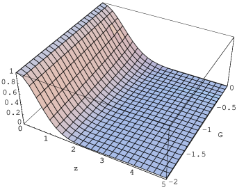
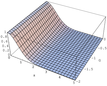
In order to give them analytical meaning one has to use methods of generalized summation. Numerical check using the Padé method (see Fig.1-2, below) shows that even low order approximants of series (20) and (22) give very good agreement with exact result calculated from (23) for G belonging to the domain much larger than the domain in which partial sums of both series give acceptable results. Moreover, comparing these results we in fact compare results given by the Padé method with exact solutions for simplified, nevertheless essentially quantum, model. This confirms practical utility of the Padé summation method applied to various perturbation expansions occurring in quantum physics even if we are unable to prove its applicability in a mathematically satisfactory way. It also confirms that generating functions obtained as solutions to the boson normal ordering problem and being in general divergent formal series may be interpreted as asymptotic expansions, resumed in such a generalized sense and, as a consequence, used in physical applications.

Acknowledgments

A.G. wishes to thank the Polish Ministry of Scientific Research and Information Technology for support under Grant No: 1P03B 060 27.

Refer to caption
Refer to caption
Figure 1: The sum of the series (23), $g=\xi=1$, (left plot) and its comparison with Padé approximants $[3,4]$ for the series (20) (dashed curve, worse approximation) and (22) (continuous curve, nondistinguishable from the plot of (23)) for $G=1$.
Refer to caption
Refer to caption
Figure 2: Subdiagonal Padé approximants $[3,4]$, $g=\xi=1$, for the series (20) (left plot) and (22) (right plot). It is seen that both approximations mimic the exact result (23) very well. It may be also checked that the results weakly depend on the order of approximation.

References

References

  • [1] Katriel J 1974 Lett. Nuovo Cim. 10 565.
  • [2] Comtet L 1974 Advanced Combinatorics, Dordrecht: Reidel.
  • [3] Blasiak P, Penson K A, Solomon A I 2003 Phys. Lett. A 309 198.
  • [4] Mendez M A, Blasiak P, Penson K A 2005 J. Math.Phys. 46 083511.
  • [5] Blasiak P 2005 Combinatorics of boson normal ordering and some applications, PhD Thesis, Institute of Nuclear Physics, Polish Academy of Sciences: Kraków and Université P. et M. Curie: Paris; Concepts of Physics 2 (2005), in press; arXiv:quant-ph/0507206
  • [6] Louisell W H 1990 Quantum Statistical Properties of Radiation, J. Wiley: New York.
  • [7] Aldrovandi R (2001) Special Matrices of Mathematical Physics (World Scientific, Singapore)
  • [8] Blasiak P, Penson K A, Solomon A I, Horzela A, Duchamp G H E 2005 J. Math.Phys. 46 052110.
  • [9] Dattoli G, Ottaviani P L, Torre A and Vàsquez L(1997) Riv. Nuovo Cim. 20 1
  • [10] Dattoli G 2000 J. Comp. and Applied Mathematics 118 111