Non-Markovian dynamics of a qubit

Abstract

In this paper we investigate the non-Markovian dynamics of a qubit by comparing two generalized master equations with memory. In the case of a thermal bath, we derive the solution of the recently proposed post-Markovian master equation [A. Shabani and D.A. Lidar, Phys. Rev. A 71, 020101(R) (2005)] and we study the dynamics for an exponentially decaying memory kernel. We compare the solution of the post-Markovian master equation with the solution of the typical memory kernel master equation. Our results lead to a new physical interpretation of the reservoir correlation function and bring to light the limits of usability of master equations with memory for the system under consideration.

I Introduction

The dynamics of systems interacting with their surroundings is in general very complicated. Very often, however, the physical systems of interest are sufficiently isolated from their environment to allow the use of certain approximations such as the weak coupling approximation and the Markovian approximation petruccionebook . The former one assumes that the interaction between the system and the environment is sufficiently weak, i.e. the system is quasi-closed. The latter one relies on the assumption that the characteristic times of the system are much longer than those of the environment, and it always assumes the validity of the weak coupling approximation.

Most of the results on open systems dynamics are based on the weak coupling and Markovian approximations. Recent studies have shown the limits of the Markovian description of quantum computation and quantum error correction Alicki02 ; Ahn ; Daffer04 ; Terhal05 ; Preskill . Moreover, nanotechnology-based devices using hybrid systems, e.g. combining quantum optical and solid state systems, have been investigated and seem to be very promising for future technological applications Tian04 ; Tian04b . In order to describe decoherence in many solid state systems non-Markovian approaches need often to be used John94 ; quang97 ; Vega05 ; Florescu04 . Finally, a comprehensive and complete understanding of the interaction between a quantum system and its environment, not relying on the weak coupling and/or Markovian approximations, is crucial in order to clarify fundamental issues such as the quantum-classical border, and in order to gain new insight in the dynamics of quantum systems which are not in thermal equilibrium.

Outside the region of validity of the Markovian approximation the master equation describing the dynamics cannot be usually cast in the well known Lindblad form Lindblad ; Gorini . This fact has several consequences: one for all, complete positivity of the dynamical map note1 is not guaranteed anymore, and even positivity may be violated. The latter of this properties, i.e. positivity, is necessary to guarantee the statistical interpretation of the density matrix, while the former one ensures that the time evolution in the system-environment total space is unitary .

Non-Lindblad master equations are much more difficult to solve, both analytically and numerically, than Lindblad ones, and they may lead to non-physical behaviors such as, e.g., violation of positivity of the dynamical map [See, e.g., Refs. Munro96 ; barnett ; Maniscalco05 ]. The break down of the positivity condition stems from the phenomenological nature of most of the non-Markovian approaches. Exact generalized master equations indeed, by definition, do not violate neither positivity nor complete positivity but they are generally far too complicated for providing useful means for studying the system dynamics.

In this paper we focus on a basic model of an open quantum system with memory, i.e. a two-level system (qubit) interacting with a bosonic thermal reservoir. We apply a recently proposed post-Markovian approach lidar05 which interpolates between the exact Kraus map and the Markovian dynamics. We compare the solution of the post-Markovian generalized master equation with the solution of the typical memory kernel master equation petruccionebook ; barnettbook . For a specific physically interesting form of the reservoir spectral density it is possible to derive an exact solution starting from a microscopic description of the total system, i.e. system plus reservoir. This fact allows us to make a comparison between the phenomenological memory kernel approaches and the exact microscopic approach. From this comparison a new physical interpretation of the reservoir correlation function will emerge. Finally the limitations of the memory kernel approaches will be underlined and issues related to the loss of positivity of the dynamical maps will be carefully analyzed.

The paper is structured as follows. In Sec. II we recall the post-Markovian master equation and we present the solution for the case of a qubit interacting with a thermal reservoir. In Sec. III we recall the solution of the typically used generalized master equation with memory, we compare it to the post-Markovian solution, and we analyze the “non-physical”region of the parameters space where positivity breaks down. In Sec. IV we consider the exact solution and in Sec. V we present conclusions.

II Post-Markovian master equation for a qubit

II.1 Interpolating the Kraus and Markovian dynamical maps

Very recently a new general post-Markovian master equation has been presented lidar05 . An interesting feature of this phenomenological master equation is that, by construction, it interpolates between the generalized measurement interpretation of the exact Kraus operator sum map, and the continuous measurement interpretation of the Markovian dynamics.

It is worth reminding that the dynamics of open quantum systems may be described equivalently either by means of the density matrix satisfying the master equation or by means of a stochastic wave function which is the solution of the stochastic Schrödinger equation unravelling the dynamics petruccionebook . For Markovian dynamics there exist a physical interpretation for the time evolution of the stochastic wave functions (quantum trajectories). Indeed it has been shown that the quantum trajectories describe the time evolution of the system conditioned to a continuous measurement of the environment carmichaelbook ; Moelmer96 . Different types of detection schemes of the environment (photon counting, homodyne and heterodyne detection) correspond to different unravellings (different types of stochastic Schrödinger equations). At contrast, in the case of non-Markovian dynamics, it has been shown that quantum trajectories do not have a physical interpretation Gambetta02 although attempts to find an interpretation in extended Hilbert states have been performed Breuer04 . In more detail, it turns out that the stochastic wave function at time $t$ represents the state the system would be in at that time if a measurement was performed on the environment at that time, and yielded a particular result (generalized measurement interpretation). However, the wavefunction at time $t$ does not have any link with itself at times less then $t$, and therefore there cannot be any physical interpretation of the quantum trajectories, for non-Markovian systems Gambetta02 . The reason can be traced back to the finite correlation time characterizing the non-Markovian bath.

Now, since the post-Markovian master equation actually interpolates between the exact dynamics and the Markovian dynamics, an analysis of the time evolution according to this equation may give new insight in the dynamics of non-Markovian systems, in the possible physical phenomena taking place when the Markovian approximation fails, and in their role in the break down of the continuous measurement interpretation. This is in fact what we are going to investigate in the rest of the paper. Moreover, we will study the usefulness of the post-Markovian master equation presented in Ref. lidar05 for the description of open quantum systems, comparing it to other common non-Markovian approaches. To this aim we consider the basic open quantum system, e.g. a two-level atom or qubit, interacting linearly with a quantized bosonic reservoir at $T$ temperature.

II.2 Post-Markovian master equation for the qubit

The general form of the post-Markovian master equation introduced in Ref. lidar05 is the following

$$\frac{d\rho}{dt}=\mathcal{L}\int_{0}^{t}dt^{\prime}k(t^{\prime})\exp(\mathcal{L}t^{\prime})\rho(t-t^{\prime}),$$ (1)

where $\rho(t)$ is the density matrix of the reduced system, $k(t^{\prime})$ is the memory kernel, and $\mathcal{L}$ is the Markovian Liouvillian. For the system here considered the Markovian Liouvillian is given by GardinerZollerbook

$$\mathcal{L}\rho = \gamma_{0}(N+1)\left[\sigma_{-}\rho\sigma_{+}-\frac{1}{2}\sigma_{+}\sigma_{-}\rho-\frac{1}{2}\rho\sigma_{+}\sigma_{-}\right]$$ (2)

$$+ \gamma_{0}N\left[\sigma_{+}\rho\sigma_{-}-\frac{1}{2}\sigma_{-}\sigma_{+}\rho-\frac{1}{2}\sigma_{-}\sigma_{+}\right],$$

with $\gamma_{0}$ the phenomenological dissipation constant, $N$ the mean number of excitations of the reservoir, and $\sigma_{\pm}$ the spin inversion operators. In Appendix A we recall the form of the solution of the Markovian master equation via the damping basis method.

In the following we will focus on a widely use form of memory kernel, namely the exponential memory kernel

$$k(t)=\gamma e^{-\gamma t}.$$ (3)

It is worth stressing that $k(t)$, which hereafter we will call the Shabani-Lidar memory kernel, is a quantity introduced phenomenologically in Ref. lidar05 . Therefore, it should not be confused with the memory function, appearing in the second order approximation of the Nakajima-Zwanzig equation, which is related to the spectral density of the reservoir [See, e.g., petruccionebook , p.465]. In order to understand the meaning of the Shabani-Lidar memory kernel we recall that, in the measurement scheme approach to open quantum systems, the post-Markovian master equation describes a situation in which a measurement of the environment at a time $t^{\prime}$ is followed by a Markovian evolution, described in terms of continuous measurements of the environment at times $t>t^{\prime}$. The time $t^{\prime}$ characterizes the bath memory effects. In this picture, the Shabani-Lidar memory kernel is a function which assigns weights to different measurements (selecting different $\rho(t^{\prime})$) lidar05 . Now, having in mind these definitions, and remembering that that the post-Markovian master equation is phenomenological, one might wonder which is the relationship between the memory kernel of the post-Markovian master equation and the Nakajima-Zwanzig memory function (also known as correlation function) which is related to the reservoir spectral density. This question will be addressed in Sec. IV.

II.3 Analytic solution

By applying the method described in lidar05 , and recalled in Appendix B, to a two-level system whose ground and excited states are $|1\rangle$ and $|2\rangle$, respectively, we derive the following solution of the post-Markovian master equation

$$\rho(t) = \frac{1}{2}\left\{I-\left[\xi(R,t)\left(\rho_{11}-\rho_{22}+\frac{1}{2N+1}\right)\right.\right.$$ (4)

$$- \left.\left.\frac{1}{2N+1}\right]\sigma_{z}+\frac{\xi(2R,t)}{2}\left[\rho_{12}\sigma_{+}+\rho_{21}\sigma_{-}\right]\right\},$$

where $\rho_{ij}=\langle i|\rho(0)|j\rangle$, with $i,j=1,2$. In the previous equation

$$\xi(R,\tau) = e^{-\frac{R+1}{2}\tau}\left\{\frac{1}{\sqrt{|1-r(R)|}}\sinh\left[\sqrt{|1-r(R)|}\frac{(R+1)\tau}{2}\right]\right.$$ (5)

$$+ \left.\cosh\left[\sqrt{|1-r(R)|}\frac{(R+1)\tau}{2}\right]\right\},$$

and

$$r(R)=\frac{4R}{(R+1)^{2}},$$ (6)

with $R=|\lambda_{2}|/\gamma$, the eigenvalue $\lambda_{2}$ being the one derived for the Markovian master equation [see Eq. (28)], and $\tau=\gamma t$.

Equation(5) is valid only for $r(R)\leq 1$ and $r(2R)\leq 1$. When $r(R)>1$ and/or $r(2R)>1$, the form of the time dependent coefficients $\xi(R,\tau)$ and/or $\xi(2R,\tau)$ appearing in Eq. (4) is obtained from Eq. (5)by substituting $\sinh[.]$ and $\cosh[.]$ with $\sin[.]$ and $\cos[.]$, respectively.

Let us focus on the case of a zero-temperature reservoir. In this case the solution of the post-Markovian master equation takes the form

$$\rho(\tau)=\frac{1}{2}\{I+\left[2P_{1}(\tau)-1\right]\sigma_{z}+\left[2\rho_{12}(\tau)\sigma_{+}+h.a.\right]\},$$ (7)

where the time evolution of the ground state population $P_{1}(\tau)=\rho_{11}(\tau)$ and of the coherences $\rho_{12}(\tau)=\rho_{21}^{*}(\tau)$ is given, respectively, by:

$$P_{1}(\tau) = \rho_{11}\xi(R,\tau),$$ (8)

$$\rho_{12}(\tau) = \frac{1}{4}\rho_{12}\xi(2R,\tau).$$ (9)

We note that, for the zero-temperature case here considered, $\lambda_{2}=-\gamma_{0}$, and therefore $R=\gamma_{0}/\gamma$.

II.4 Markovian limit

We conclude this section by showing the Markovian limit of the post-Markovian solution. To this aim we firstly notice that Eq. (5) can be recast in the following simplified form

$$\xi(R,t) = \frac{e^{-|\lambda_{2}|t}-Re^{-\gamma t}}{1-R}.$$ (10)

For times $t\gg 1/\gamma\equiv\tau_{R}$ (coarse graining in time) and for $R\ll 1$, i.e. $\tau_{0}=1/\gamma_{0}\gg\tau_{R}$, the previous equations become $\xi(R,t)\simeq e^{-|\lambda_{2}|t}$, while $\xi(2R,t)\simeq e^{-2|\lambda_{2}|t}$, and one reobtains the Markovian dynamics. The approximation $\tau_{0}=1/\gamma_{0}\gg\tau_{R}$ amounts at saying that $\tau_{R}$ is much smaller than the characteristic time of the system $\tau_{0}$. In the following we will call $\tau_{R}$ the characteristic time of the reservoir.

III Generalized master equation with memory

III.1 Phenomenological master equation

Let us now consider the typical phenomenological master equation with memory kernel having the form

$$\frac{d\rho}{dt}=\int_{0}^{t}dt^{\prime}k(t^{\prime})\mathcal{L}\rho(t-t^{\prime}).$$ (11)

This generalized master equation takes into account the previous “history”($0<t^{\prime}<t$) of the density matrix $\rho(t)$ by means of the phenomenological memory kernel $k(t^{\prime})$. Differently from time-convolutionless approaches petruccionebook , this leads to a master equation which is not local in time. For specific forms of the memory kernel, as the exponential one considered in this paper, this master equation can be solved by means of the Laplace transforms.

The memory kernel master equation given by Eq. (11) has been used in Ref. barnett for studying the non-Markovian dynamics of a quantum harmonic oscillator interacting with the vacuum. There the authors have found that, for an exponential memory kernel such as the one given by Eq. (3), the positivity of the density matrix is violated for certain values of the phenomenological decay constants. In Ref. Daffer04 the generalized master equation with memory given in Eq. (11) has been analyzed for a two-level atom in the presence of telegraphic noise, and conditions for complete positivity have been presented. In the present paper we consider this model for the two-level atom interacting with a bosonic reservoir at $T$ temperature, focussing in particular, for the sake of simplicity, on the zero temperature reservoir.

Similarly to the case of the post-Markovian master equation, one can solve Eq. (11) by taking its Laplace transform, determining the poles, and inverting the solution in the standard way. Using the damping basis given by Eq. (27), with the eigenvalues given by Eq. (28), we find that the solution has the same form of Eq. (4), with the only difference that the quantities $\xi(R,t)$ is now given by

$$\xi(R,\tau) = e^{-\frac{\tau}{2}}\left\{\frac{1}{\sqrt{|1-4R|}}\sinh\left[\frac{\tau}{2}\sqrt{|1-4R|}\right]\right.$$ (12)

$$+ \left.\cosh\left[\frac{\tau}{2}\sqrt{|1-4R|}\right]\right\}.$$

By comparing Eq. (5) and Eq. (12), with the help of Eq. (6), one easily sees that this amounts at assuming $R=\gamma_{0}/\gamma\ll 1$ in Eq. (5). Stated another way, as one can see directly form Eqs. (1) and (11), the memory kernel master equation is a special case of the post-Markovian master equation, in the limit in which the system characteristic time $\tau_{0}$ is much bigger than the reservoir correlation time $\tau_{R}$ lidar05 . We note that, for $4R>1$ and $8R>1$ the form of the time dependent coefficients $\xi(R,\tau)$ and/or $\xi(2R,\tau)$, respectively, is obtained from Eq. (12) by substituting $\sinh[.]$ and $\cosh[.]$ with $\sin[.]$ and $\cos[.]$.

We conclude this section noting that, as for the Markovian dynamics, the solution of the master equation with memory, given by Eq. (11), can be obtained from the solution of the post Markovian master equation in the limit $R=\gamma_{0}/\gamma\ll 1$. However, contrarily to the Markovian dynamics, no coarse graining in time has been made, and therefore the solution of Eq. (11) describes correctly the short time dynamics, $t\ll\tau_{R}$, characterized by non-negligible system-reservoir correlations.

III.2 Positivity of the dynamical map

As we have already mentioned in the Introduction, since the master equations given by Eqs. (1) and (11) are not of Lindblad-type, the positivity of their corresponding dynamical maps is not guaranteed. The break down of the positivity condition means that the density matrix loses its statistical interpretation, its eigenvalues becoming negative. This is hence a sign of failure of the phenomenological master equations with memory.

An analysis of the positivity condition for a master equation of the form of Eq.(11) has been presented, in the case of a damped harmonic oscillator, in Ref. barnett . There the authors have found that positivity is always violated for sufficiently high values of the phenomenological decay constant. The positivity condition of the memory kernel master equation has been also studied in Ref. Budini04 for different types of memory kernels, including the exponential one, generalizing the results of barnett . It is therefore not surprising that, as we will see in the following, we obtain the same result of Ref. barnett for the same form of master equation, with an exponential memory kernel, when the system is a qubit. As we will show, however, the post-Markovian master equation exhibits a strikingly different behavior in respect of the positivity condition.

In order to study in more detail the positivity condition for both the two memory kernel master equations considered in this paper, it is more convenient to rewrite the solutions in terms of the Bloch vector $\vec{w}=\{w_{x},w_{y},w_{z}\}$. The qubit density operator at time $\tau=\gamma t$, given by Eqs.(4) and Eq. (5) in the post-Markovian case, and by Eqs.(4) and (12) in the memory kernel case, can be recast in the form

$$\rho(\tau)=\frac{1}{2}\left[I+\vec{w}(\tau)\cdot\vec{\sigma}\right],$$ (13)

with $\vec{\sigma}=\{\sigma_{x},\sigma_{y},\sigma_{z}\}$, and

$$w_{x}(\tau) = \xi(2R,\tau){\rm Re}[\rho_{12}]=\xi(2R,\tau)w_{x}(0)$$ (14)

$$w_{y}(\tau) = -\xi(2R,\tau){\rm Im}[\rho_{12}]=\xi(2R,\tau)w_{y}(0)$$ (15)

$$w_{z}(\tau) = 2P_{1}\xi(R,\tau)-1=P_{1}(\tau)-P_{2}(\tau),$$ (16)

where $P_{1}(\tau)$ is given by Eq.(8), $P_{2}(\tau)=1-P_{1}(\tau)$, and $\xi(R,\tau)$ is given by Eq. (12) (post-Markovian) or Eq. (5) (memory kernel). The dynamical map describing the evolution of the qubit is positive if and only if the density operator evolves only to states inside or on the Bloch sphere. Therefore the positivity condition, in terms of the Bloch vector components, simply reads $|w_{i}(\tau)|\leq 1$, $i=x,y,z$. By looking at Eqs. (14)-(16) and Eq.(8), one sees immediately that the conditions $|w_{i}(\tau)|\leq 1$ are equivalent to $|\xi(R,\tau)|\leq 1$ and $|\xi(2R,\tau)|\leq 1$.

Let us begin considering the post-Markovian master equation. It is straightforward to prove that $\xi(R,\tau)$ is a positive and monotonically decreasing function of $R$, therefore, it is sufficient to investigate the conditions for which $|\xi(R,\tau)|\leq 1$, since $|\xi(2R,\tau)|\leq|\xi(R,\tau)|$ for all values of $R$ and $\tau$. As shown in Appendix C, it turns out that the post-Markovian dynamical map never violates positivity. On the contrary, for the case of the memory kernel master equation given by Eq. (11), a close look to Eq. (12) tells us that $|\xi(R,\tau)|\leq 1$ only for $4R<1$, i.e. $4\gamma_{0}<\gamma$. We remind that one may derive the memory kernel master equation given by Eq. (11) from the post-Markovian master equation given by Eq. (1) in the limit $\gamma_{0}\ll\gamma$. Having this is mind it is not surprising that the positivity condition breaks down for sufficiently high values of $\gamma_{0}$, for the system here considered. The study of positivity, therefore, suggests that the post-Markovian master equation is somehow “more fundamental”than the memory kernel master equation.

IV Exact dynamics

In this section we will analyze two different aspects characterizing the non-Markovian dynamics of a quibit described by means of memory kernel master equations. The first aspect stems from the microscopic derivation, using the Nakajima-Zwanzig formalism, of the phenomenological memory kernel master equation given by Eq. (11). The microscopic derivation will allow us to link the Shabani-Lidar memory kernel to the correlation function and to the reservoir spectral density, in the limit $\gamma_{0}\ll\gamma$.

The second aspect described in this section is related to a physically interesting specific microscopic model of non-Markovian dynamics of a qubit for which an exact solution does exist. The existence of an exact solution allows to make a comparison with the predictions of the post-Markovian and memory kernel solutions, and hence to study the limits of both these approaches. Moreover, keeping in mind that the post-Markovian approach can be seen as an interpolation between the exact Kraus map and the Markovian one, one may gain new insight in the reason why non-Markovian quantum trajectories lack of a physical meaning.

IV.1 Microscopic derivation

Let us begin with the microscopic derivation of the memory kernel master equation given by Eq. (11) . We consider the following microscopic Hamiltonian for the total system, i.e. system plus reservoir,

$$H=H_{0}+H_{I},$$ (17)

with

$$H_{0} = \frac{\hbar\omega_{0}}{2}\sigma_{z}+\sum_{k}\omega_{k}b^{{\dagger}}_{k}b_{k},$$

$$H_{I} = \sigma_{+}B+\sigma_{-}B^{{\dagger}},$$ (18)

where $B=\sum_{k}g_{k}b_{k}$. The transition frequency of the two-level system is denoted by $\omega_{0}$, the index $k$ labels the different modes of the reservoir with frequencies $\omega_{k}$, $b^{{\dagger}}_{k}$ and $b_{k}$ indicate the creation and annihilation operators, and $g_{k}$ are the coupling constants. Following the typical approach for the derivation of master equations for the reduced density matrix we firstly write the von Neumann master equation for the total system in the interaction picture, then we trace over the environmental degrees of freedom, under the assumptions that ${\rm Tr}_{R}\left[H_{I}(t),\rho_{T}(0)\right]=0$, with $\rho_{T}$ the density matrix of the total system, and $\rho_{T}(0)=\rho(0)\otimes\rho_{R}(0)$, with $\rho_{R}(0)$ the density matrix of the reservoir. To the second order in perturbation theory (Born approximation), we obtain the following integro-differential equation for the reduced density matrix

$$\frac{d\rho(t)}{dt}=\int_{0}^{t}dt^{\prime}{\rm Tr}_{R}\left[H_{I}(t),[H_{I}(t^{\prime}),\rho(t^{\prime})\otimes\rho_{R}]\right].$$ (19)

Having in mind Eq.(18) it is then straightforward to recast Eq.(19) in the same form of Eq. (11) with

$$k(t^{\prime}) = {\rm Tr}_{R}\left[B(0)B^{{\dagger}}(t^{\prime})\rho_{R}\right]$$ (20)

$$\equiv \int d\omega J(\omega)e^{i(\omega-\omega_{0})t^{\prime}}.$$

In the previous equation $B(t)=\sum_{k}g_{k}b_{k}\exp(-i\omega_{k}t)$ is the reservoir operator appearing in Eq. (18), in the interaction picture, and $J(\omega)=\sum_{k}g_{k}^{2}\delta(\omega-\omega_{k})/(2m_{k}\omega_{k})$, with $m_{k}$ masses of the oscillators of the reservoir. From the previous definition of $k(t^{\prime})$ one sees clearly that this function describes temporal correlations of the reservoir operators $B$, and therefore it is commonly known as the reservoir correlation function. In the second line of Eq. (20) we have introduced the so-called spectral density of the reservoir $J(\omega)$, which is therefore simply the Fourier transform of the correlation function. An exponential correlation function of the form of Eq. (3) corresponds to a Lorentzian spectral density as the one typical of cavity quantum electrodynamics, for a reservoir in the vacuum state.

In the rest of this section we will focus on the following specific physical system: a two level atom interacting resonantly with a quantized mode of an empty high Q cavity. Assuming that the two-level atom is in resonance with the cavity mode, the reservoir spectral density is the following

$$J(\omega)=\frac{1}{\pi}\frac{\bar{\gamma_{0}}\bar{\lambda}^{2}}{(\omega_{0}-\omega)^{2}+\bar{\lambda}^{2}}.$$ (21)

Using Eq. (20), we get

$$k(t^{\prime})=\bar{\gamma}_{0}\bar{\lambda}e^{-\bar{\lambda}t},$$ (22)

and the master equation (19) becomes

$$\frac{d\rho}{dt}=\int_{0}^{t}dt^{\prime}\bar{\mathcal{L}}k(t^{\prime})\rho(t-t^{\prime}),$$ (23)

with $k(t^{\prime})$ given by Eq. (22), and $\bar{\gamma}_{0}\bar{\mathcal{L}}=(\bar{\gamma}_{0}/\gamma_{0})\mathcal{L}$ , where $\mathcal{L}$ is given by Eq. (2), with $N=0$. A direct comparison with Eqs. (3) and (11) clearly shows that the master equation derived using second order perturbation theory starting from the microscopic description above coincides with the phenomenological memory kernel master equation given by Eq.(11), provided that $\bar{\lambda}=\gamma$, $\bar{\gamma}_{0}=\gamma_{0}$.

IV.2 Physical interpretation of the system and reservoir parameters

The microscopic derivation allows to give a physical interpretation of the decay constants $\gamma_{0}$ and $\gamma$. Indeed, Eq. (21) tells us that $\gamma_{0}$ measures the strength of coupling between the two-level atom and the vacuum reservoir, and hence the system characteristic time $\tau_{0}$ is determined only by the system-reservoir coupling strength. The reservoir correlation time $\tau_{R}=1/\gamma$ is simply given by the inverse of the width of the Lorentzian spectral density.

Having this in mind, the reason of the violation of positivity for the master equation given by Eq. (11) becomes clear. Indeed, such master equation correctly describes the dynamics of the system only when second order perturbation theory is valid, i.e. for weak system-reservoir coupling. The conditions in correspondence of which positivity is violated, i.e. when $4R>1$ and $8R>1$, with $R=\gamma_{0}/\gamma$, however, correspond to strong couplings between system and reservoir.

Finally, we remind that, as noticed in Sec. III.1, Eq.(19) is the limit for $\gamma_{0}/\gamma\ll 1$ of the post-Markovian master equation given by Eq.(1). As a consequence, in this limit, the Shabani-Lidar phenomenological memory kernel $k(t^{\prime})$ coincides with the Fourier transform of the reservoir spectral density, as given by Eq. (20). This fact allows to give a new physical interpretation to the correlation function of the reservoir in terms of generalized measurement by the environment. Indeed, it turns out that the reservoir correlation function acts as a weighting time distribution function, assigning weights to different measurements selecting different $\rho(t^{\prime})$.

IV.3 Exact solution

The physical system we consider in this section is one of the few open quantum systems amenable of an exact solution Garraway97 . For a spectral density of the type given by Eq. (21), the exact density matrix has the following form petruccionebook

$$\rho(t)=\begin{pmatrix}P_{1}(\tau)&\rho_{12}(\tau)\\ \rho_{12}^{*}(\tau)&1-P_{1}(\tau)\end{pmatrix},$$ (24)

with

$$P_{1}(\tau) = P_{1}(0)e^{-\tau}\Big{\{}\cosh\left[\sqrt{|1-2R|}\;\frac{\tau}{2}\right]$$ (25)

$$+ \frac{1}{\sqrt{|1-2R|}}\sinh\left[\sqrt{|1-2R|}\;\frac{\tau}{2}\right]\Big{\}}^{2},$$

for $2R\leq 1$. If $2R>1$, $P_{1}(t)$ has the same form of Eq. (25) provided that the substitutions $\cosh[.]\rightarrow\cos[.]$ and $\sinh[.]\rightarrow\sin[.]$ are made. In Fig.1 we compare the time evolution of the exited state population as predicted by both the post-Markovian master equation [see Eqs. (8) and (5)] and by the memory kernel master equation [see Eqs. (8) and (12)] with the exact dynamics [see Eq. (25)], in correspondence to three different values of the parameter $R=\gamma_{0}/\gamma$. We assume that the initial state of the two-level system is the exited state.

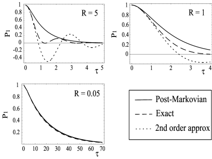
Figure 1: Time evolution of the excited state probability for three different values of $R$, i.e. $R=5$, $R=1$, $R=0.05$. The dimensionless time is $\tau=\gamma t$. The solid line indicates the dynamics for the post-Markovian master equation, the dashed lines indicates the exact dynamics and the dotted line the dynamics of the memory kernel master equation derived using second order perturbation theory.

From the figure one can see that while the memory kernel approximated dynamics does violate positivity for strong enough couplings ($R=5$ and $R=1$), the post-Markovian dynamics is always positive. However, both the post-Markovian solution and the second-order solution approximate well at all times $\tau$ the exact dynamics only for small values of $R$, e.g. for small couplings. Therefore, the specific example here considered shows that there exist situations for which there is actually no advantage in using the post-Markovian approach when compared to second order perturbation theory. The reason why the post-Markovian approach fails in describing the dynamics of the system even for intermediate couplings is related to the way in which such a master equation is derived. Let us recall the physical meaning of the post-Markovian approach in terms of generalized measurement interpretation. The derivation of the post-Markovian master equation assumes that, after the time $t^{\prime}$ at which the generalized measurement by the environment is performed, the evolution of the system is Markovian. The time distribution of the instants $t^{\prime}$ at which the measurement is performed is given by the memory kernel. Therefore one should expect such master equation to be valid for $\tau_{0}>\tau_{R}$. Indeed, for $\tau_{0}\leq\tau_{R}$ the assumption that the dynamics after $t^{\prime}$ is Markovian would not be well justified since the reservoir correlation time would then be longer than the Markovian dissipation time, and this would inevitably lead to a non-negligible feedback of the environment to the system. We see from Eq. (25) that already for $R=\gamma_{0}/\gamma\geq 0.5$ the exact dynamics of $P_{1}(\tau)$ shows an oscillatory behavior. These oscillations may be seen, in a completely quantum approach, as virtual absorption and re-emission of the same quantum of energy from the environment. The description of these quantum phenomena cannot be present in the post-Markovian approach. It is exactly the appearance of these virtual exchanges of energy which does not allow to give a physical interpretation to the single trajectories for strongly non-Markovian systems, since there seems to be no way for a single physical trajectory to describe a virtual process.

V Summary and Conclusions

In this paper we have taken into consideration two models of generalized master equations with memory, and we have applied them to the description of the non-Markovian dynamics of a qubit interacting with a quantized bosonic reservoir in thermal equilibrium. For the case of an exponential memory kernel we have compared the solution of the recently proposed post-Markovian master equation with the solution of the typical master equation with memory kernel. We have demonstrated that, for the system considered, the post-Markovian approach never violates positivity, contrarily to the memory kernel master equation. We have then seen that the memory kernel master equation coincides with the second order expansion of the exact Nakajima-Zwanzig generalized master equation. Since the memory kernel master equation is the limit of the post-Markovian master equation for $\gamma_{0}\ll\gamma$, it is possible to give a generalized measurement interpretation to the correlation function of the reservoir. Finally we have considered the following physical implementation of the system: the qubit describes the excited and ground electronic state of an effective two-level atom crossing a high $Q$ cavity; the reservoir is formed by the quantized modes of the high $Q$ cavity which are distributed according to a Lorentzian peaked at the atomic Bohr frequency. This physical system, typical of cavity QED, represents one of the few examples of exactly solvable open quantum systems. The comparison between the exact dynamics and the post-Markovian and memory kernel solutions shows that there exist situations in which the post-Markovian approach does not present any advantage over the second order approximated memory kernel master equation. The reason is traceable back to the fact that, by derivation, the post-Markovian master equation cannot describe accurately situations for which the characteristic time of the reservoir $\tau_{R}$ is greater than the characteristic time of the system $\tau_{0}$. When $\tau_{R}\geq\tau_{0}$ the dynamics is characterized by virtual exchanges of energies between the system and the environment which cannot be described by the post-Markovian approach. Such virtual processes, absent in the Markovian dynamics, seem to be responsible for the lack of a physical interpretation of single quantum trajectories in terms of continuous measurements performed by the environment.

VI Acknowledgements

S.M. thanks Nikolay Vitanov for the hospitality at the University of Sofia, where part of the work was done, and acknowledges financial support by the European Union’s Transfer of Knowledge project CAMEL (Grant No. MTKD-CT-2004-014427) and by the Angelo Della Riccia Italian National Foundation.

Appendix A

The damping basis method allows to solve the master equation given by Eq.(2) by solving the eigenvalue equation

$$\mathcal{L}\rho_{\lambda}=\lambda\rho_{\lambda}.$$ (26)

It turns out that the damping basis is Briegel93

$$\rho_{\lambda_{i}}:\{\rho_{\lambda_{1}}=\sigma_{0},\rho_{\lambda_{2}}=\sigma_{z},\rho_{\lambda_{3}}=\sigma_{+},\rho_{\lambda_{4}}=\sigma_{-}\},$$ (27)

with $\sigma_{0}=\frac{1}{2}[I-\sigma_{z}/(2N+1)]$, $\sigma_{\pm}=\sigma_{x}\pm i\sigma_{y}$, and $\sigma_{x},\sigma_{y},\sigma_{z}$ the Pauli matrices. The corresponding eigenvalues are

$$\lambda_{i}:\{\lambda_{1}=0,\lambda_{2}=-2\gamma_{0}(N+1/2),\lambda_{3}=\lambda_{4}=-\gamma_{0}(N+1/2)\}.$$ (28)

The density matrix $\rho(t)$ can then be written, in the damping basis, as follows

$$\rho(t)=\sum_{\lambda_{i}}c_{\lambda_{i}}e^{\lambda_{i}t}\rho{\lambda_{i}},$$ (29)

with $c_{\lambda_{i}}={\rm Tr\left\{\check{\rho}_{\lambda_{i}}\rho(0)\right\}}$, where $\check{\rho}_{\lambda_{i}}$ is the dual damping basis. Inserting the values of Eqs. (27)-(28) into Eq. (29), one gets

$$\rho(t) = \frac{1}{2}\left\{I-\left[e^{-\gamma_{0}(2N+1)t}\left(\rho_{11}-\rho_{22}+\frac{1}{2N+1}\right)\right.\right.$$ (30)

$$- \left.\left.\frac{1}{2N+1}\right]\sigma_{z}+\frac{e^{-\gamma_{0}(N+1/2)t}}{2}\left[\rho_{12}\sigma_{+}+\rho_{21}\sigma_{-}\right]\right\}.$$

Appendix B

In this Appendix we recall the main steps to derive the general solution of Eq. (1), as demonstrated in lidar05 , and we carry out the derivation for the case of a qubit interacting with a quantized thermal reservoir. The initial step to solve the post-Markovian master equation is the derivation of the damping basis for the Markovian case (see Appendix A). As in the previous Appendix, we denote with $\{\lambda_{i}\}$ the complex eigenvalues and with $\{\rho_{\lambda_{i}}\}$ and $\{\check{\rho}_{\lambda_{i}}\}$ the damping basis and its dual, respectively. Then we write the density matrix as follows

$$\rho(t)=\mu_{i}(t)\rho_{\lambda_{i}}.$$ (31)

Taking the Laplace transform of Eq.(1) one gets

$$s\tilde{\rho}(s)-\rho(0)=\left[\tilde{k}(s)\ast\frac{\mathcal{L}}{s-\mathcal{L}}\right]\tilde{\rho}(s),$$ (32)

where $\ast$ denotes the convolution. Taking the Laplace transform of Eq. (31) and using the previous equation one obtains

$$s\tilde{\mu}_{i}(s)-\mu_{i}(0)=\lambda_{i}\tilde{k}(s-\lambda_{i})\tilde{\mu}_{i}(s),$$ (33)

and transforming back

$$\mu_{i}={\rm Lap}^{-1}\left[\frac{1}{s-\lambda_{i}\tilde{k}(s-\lambda_{i})}\right]\mu_{i}(0)\equiv\xi_{i}(t)\mu_{i}(0).$$ (34)

The coefficients $\xi_{i}$ may be calculated once fixed $\mathcal{L}$ and $k(t)$ (see lidar05 ), therefore one gets

$$\rho(t)=\sum_{i}\xi_{i}(t)\mu_{i}(0)\rho{\lambda_{i}}.$$ (35)

For the case of a qubit interacting with a $T$-temperature reservoir, the damping basis is given by Eq. (27). Assuming an exponential memory kernel, and using Eq. (28), we have solved Eq. (34) obtaining

$$\xi_{1}(t) = 1,$$

$$\xi_{2}(t) = \xi(R,t),$$

$$\xi_{3}(t) = \xi_{4}(t)=\xi(2R,t),$$ (36)

with $\xi(R,t)$ given by Eq. (5). Inserting the previous equations into Eq. (35), one gets Eq. (4).

Appendix C

In this Appendix we demonstrate that the post-Markovian master equation for a qubit never violates the positivity condition for an exponential memory kernel. We have seen in Sec. III.2 that the positivity condition amounts at $0\leq\xi(R,\tau)\leq 1$.

Let us firstly show that $\xi(R,\tau)\leq 0$. By looking at Eq. (10), and remembering that for the zero temperature case $|\lambda_{2}|=\gamma_{0}$, one sees immediately that this corresponds to prove that

$$\left\{\begin{matrix}1-R>0,&\hskip 28.45274pte^{-R\tau}-Re^{-\tau}>0;\\ 1-R<0,&\hskip 28.45274pte^{-R\tau}-Re^{-\tau}<0.\end{matrix}\right.$$ (37)

The first set of inequalities is always satisfied since when $R<1$ then $e^{(1-R)\tau}>R$ at all times $\tau$. Similarly the second set of inequalities is always satisfied since when $R>1$ then $e^{-(R-1)\tau}\leq 1<R$ at all times $\tau$.

We now show that $\xi(R,\tau)\leq 1$. Since $R>0$ and $\xi(R,\tau)\geq 0$ we have

$$\xi(R,\tau)=\frac{e^{-R\tau}-Re^{-\tau}}{1-R}\leq\frac{e^{-\tau}-Re^{-\tau}}{1-R}=e^{-\tau}\leq 1.$$ (38)

References

- (1) H.-P. Breuer and F. Petruccione, The Theory of Open Quantum systems (Oxford University Press, 2002).
- (2) R. Alicki et al., Phys. Rev. A 65, 062101 (2002); R. Alicki et al., Phys. Rev. A 70, 010501 (2004).
- (3) D. Ahn et al., Phys. Rev. A 66, 012302 (2002); D. Ahn et al., Phys. Rev. A 70, 024301 (2004).
- (4) S. Daffer et al., Phys. Rev. A 70, 010304 (2004).
- (5) B.M. Terhal and G. Burkard, Phys. Rev. A 71, 012336 (2005).
- (6) P. Aliferis, D. Gottesman, and J. Preskill, eprint quant-ph/0504218.
- (7) L. Tian et al, Phys. Rev. Lett. 92, 247902 (2004).
- (8) L. Tian and P. Zoller, Phys. Rev. Lett. 93, 266403 (2004).
- (9) S. John and T. Quang, Phys. Rev. Lett. 74, 3419 (1994).
- (10) T. Quang et al, Phys. Rev. Lett. 79, 5238 (1997).
- (11) I. de Vega, D. Alonso, and P. Gaspard, Phys. Rev. A 71, 023812 (2005).
- (12) L. Florescu et al., Phys. Rev. A 69, 013806 (2004).
- (13) G. Lindblad, Commun. Math. Phys. 48, 119 (1976).
- (14) V. Gorini, A. Kossakowski, and E.C.G. Sudarshan, J. Math. Phys. 17, 821 (1976).
- (15) A map is completely positive iff satisfies both (positivity condition) and , with the -dimensional identity operator.
- (16) W.J. Munro and C.W. Gardiner, Phys. Rev. A 53, 2633 (1986).
- (17) S.M. Barnett and S. Stenholm, Phys. Rev. A 64, 033808 (2001).
- (18) S. Maniscalco, Phys. Rev. A 72, 024103 (2005).
- (19) A. Shabani and D.A. Lidar, Phys. Rev. A 71, 020101(R) (2005).
- (20) S.M. Barnett and P.M. Radmore Methods in Theoretical Quantum Optics (Oxford University Press, Oxford, 1997).
- (21) H.J. Carmichael, An Open Systems Approach to Quantum Optics (Springer-Verlag, Berlin, 1993).
- (22) K. Mølmer and Y. Castin, Quantum Semiclass. Opt. 8, 49-72 (1996).
- (23) J. Gambetta and H.M. Wiseman, Phys.Rev. A 66, 012108 (2002).
- (24) H.-P. Breuer, Phys. Rev. A 70, 012106 (2004).
- (25) C.W. Gardiner and P. Zoller, Quantum Noise (Springer-Verlag, Berlin, 2000).
- (26) A.A. Budini, Phys. Rev. A 69, 042107 (2004).
- (27) B.M. Garraway, Phys. Rev. A 55, 2290 (1997).
- (28) H.-J. Briegel and B.-C. Englert, Phys. Rev. A 47, 3311 (1993).