Quantum Algorithm for Commutativity Testing of a Matrix Set

Abstract

Suppose we have $k$ matrices of size $n\times n$. We are given an oracle that knows all the entries of $k$ matrices, that is, we can query the oracle an $(i,j)$ entry of the $l$-th matrix. The goal is to test if each pair of $k$ matrices commute with each other or not with as few queries to the oracle as possible. In order to solve this problem, we use a theorem of Mario Szegedy [Sze04b, Sze04a] that relates a hitting time of a classical random walk to that of a quantum walk. We also take a look at another method of quantum walk by Andris Ambainis [Amb04a]. We apply both walks into triangle finding problem [MSS05] and matrix verification problem [BS05] to compare the powers of the two different walks. We also present Ambainis’s method of lower bounding technique [Amb00] to obtain a lower bound for this problem. It turns out Szegedy’s algorithm can be generalized to solve similar problems. Therefore we use Szegedy’s theorem to analyze the problem of matrix set commutativity. We give an $O(k^{4/5}n^{9/5})$ algorithm as well as a lower bound of $\Omega(k^{1/2}n)$. We generalize the technique used in coming up with the upper bound to solve a broader range of similar problems. This is probably the first problem to be studied on the quantum query complexity using quantum walks that involves more than one parameter, here, $k$ and $n$.

Chapter 1 Introduction

1.1 The Model, Motivation, and the Main Results

Suppose we are given a set $X$ of size $n$ and we want to test if the set satisfies a given property. We are also given an oracle that computes $f(i)$ for some index $i$ in the set. For example, in element distinctness [Amb04a], $X$ is a set of integer variables, $\{x_{1},x_{2},\ldots,x_{n}\}$ and the property to test is whether there are two different indices $i$ and $j$ such that $x_{i}=x_{j}$. In order to decide if $X$ satisfies the property, we query the oracle for values $f(i)=x_{i}$ at various indices $i$. In general, we are interested in minimizing the classical or quantum query complexity, the number of queries a classical or quantum algorithm make to the oracle. This notion will be defined formally in Section 1.2.5.

We are interested in studying classical and quantum query complexities because an oracle sometimes gives a separation between them. For example, de Beaudrap, Cleve and Watrous showed one problem where we need an exponentially many queries in the bounded error classical case, but only a single query is needed in the quantum case [dBCW]. Another occasion to study a query complexity is when obtaining a time complexity is hard. In such a case, the number of queries we make gives a lower bound for the time complexity. In fact, currently there is no lower bound method for quantum time complexity that gives super-linear bounding, and by studying quantum query complexity, we get lower bounds heuristic on quantum time complexity.

One of the powers of quantum computation comes from the fact that we can query in superposition. That is, if we are given a set of $n$ elements from $1$ to $n$ denoted $[n]$, we can query an oracle in parallel once to obtain a superposition of $f(1)$ through $f(n)$. However, as we will see in Section 1.2.2, we can in a sense only learn one of the $f(i)$’s from such a query. The real power of quantum computation comes from interference. That is, the information in the states, e.g., $f(i)$’s, can be combined by means of unitary quantum gates in a non-trivial way, and we can extract a global property of the inputs. For example, in Deutsch’s algorithm, given two input bits indexed by $0$ and $1$, we cannot obtain both $f(0)$ and $f(1)$ in one oracle query. However, by making a suitable quantum query, we can obtain a global property, $f(0)\oplus f(1)$ [Deu85]. This interference is also used for quantum search in an unstructured database, in an algorithm due to Grover [Gro98], to extract a global property, i.e., if the set we are given contains an element we are looking for.

It turns out we can generalize Grover’s search to test if a set we have satisfies a given property using a quantum version of a random walk, called a quantum walk. Using a quantum walk, for example, element distinctness can be solved in $O(n^{2/3})$ [Amb04a] queries with a matching lower bound of $\Omega(n^{2/3})$ [AS04]. A quantum walk was first studied on the line, both discrete [ABN⁺01] and continuous [FG98], analogous to classical discrete and continuous random walks, except that a quantum discrete walk uses a coin to decide which point to move to next, whereas a quantum continuous walk does not. The discrete quantum walk on the line showed that the probability distribution after certain number of steps of quantum walk is different from that of the classical probability distribution [ABN⁺01]. The continuous quantum walk was then applied to a graph that gave an exponential speed up in a hitting time as compared to the classical counterpart [CFG02]. The discrete quantum walk on the line was also extended to general graphs [AAKV01] and later applied to a search on a hypercube [SKW03]. Both discrete [AKR05] and continuous [CG04] walks were applied to search an item on a grid. Ambainis [Amb04a] used a discrete quantum walk to solve element distinctness. This is generalized in [MSS05] to find a three clique in a graph (triangle finding). Szegedy proposed a different quantization of a classical Markov chain in [Sze04b, Sze04a]. He showed that there is a quadratic speedup for the hitting time of his quantization of classical walk. Szegedy’s quantization was applied in [BS05] to verify a product of two matrices (matrix verification). For more details in the development of quantum walk based algorithms, see [Amb04b].

The goal of this essay is to investigate the query complexity of testing the commutativity of $k$ matrices of size $n\times n$. This essay is probably the first to study quantum query complexity that involves two variables, $k$, the number of matrices in the set and $n$, their dimension. We show that there are three upper bounds for this problem, $O(kn^{5/3})$, $O(k^{2/3}n^{2})$ and $O(k^{4/5}n^{9/5})$, depending on the relationships between the variables $k$ and $n$. We also show a lower bound of $\Omega(k^{1/2}n)$.

The organization of the essay is as follows. We first introduce the mathematical background necessary to understand our quantum algorithms in Section 1.2. Then we take a look at the details of Szegedy-Walk in Section 2.1 and Ambainis-Walk in Section 2.2. We use these two walks to analyze triangle finding problem in Section 2.3 to see a case where Amabinis-Walk performs better. In Section 2.4.1, we take a look at a quantum adversary method [Amb00] to obtain a lower bound for our problems. We shift our focus to matrices next and in Section 2.5, we study matrix verification problem. In Chapter 3, we finally study the problem of testing the commutativity of $k$ matrices of size $n\times n$. We first take a look at a case where $k=2$ by using a modification of matrix verification in Section 3.1. Next we study four different algorithms for a general $k$ in Section 3.2. This problem is generalized in Section 3.3. Finally we give a summary and directions for future work in Chapter 4.

1.2 Mathematical Background

In this section, we will go over the mathematical background necessary to follow the algorithms in this essay. Beyond the content in this section, [NC00] is a good reference in general introductory material in quantum computation.

1.2.1 Space and qubit

Classically, information is encoded in a binary string using a sequence of bits $0$ and $1$. Quantumly, information is encoded in a finite-dimensional complex vector space, endowed with the standard inner product, a Hilbert space using qubits. A qubit may exist in states $|0\rangle$ and $|1\rangle$, which are basis vectors for a two-dimensional space.

$$|0\rangle=\left(\begin{array}[]{c}1\\ 0\\ \end{array}\right)$$

and

$$|1\rangle=\left(\begin{array}[]{c}0\\ 1\\ \end{array}\right),$$

or in any linear combination of these basis states with unit norm. We call the two vectors $|0\rangle$ and $|1\rangle$ computational basis for the two-dimensional Hilbert space since they correspond to the conventional bit representation of information. There are other pairs of basis states that span the two-dimensional Hilbert space but we focus on the computational basis. The state of a sequence of $n$ qubits is a unit vector in the $n$-fold tensor product space ${\mathbb{C}}^{2}\otimes{\mathbb{C}}^{2}\otimes\ldots\otimes{\mathbb{C}}^{2}$. This $2^{n}$-dimensional space is spanned by tensor products of states $|0\rangle$, $|1\rangle$. This is the computational basis for the $n$-qubit memory. The tensor product of two vectors $|\phi\rangle$ and $|\psi\rangle$ is denoted as $|\phi\rangle\otimes|\psi\rangle$. When these are computational basis vectors given by bit strings $x,y$, we may abbreviate the state $|x\rangle\otimes|y\rangle$ by $|x,y\rangle$ or simply $|xy\rangle$. The latter two make sense when $x$ and $y$ are bit-strings. Using a standard vector notation, a tensor product of two vectors is obtained by multiplying each entry in the left vector with the right vector.

$$\left(\begin{array}[]{c}a\\ b\\ \end{array}\right)\bigotimes\left(\begin{array}[]{c}c\\ d\\ e\\ \end{array}\right)=\left(\begin{array}[]{c}a\left(\begin{array}[]{c}c\\ d\\ e\\ \end{array}\right)\\ b\left(\begin{array}[]{c}c\\ d\\ e\\ \end{array}\right)\\ \end{array}\right)=\left(\begin{array}[]{c}ac\\ ad\\ ae\\ bc\\ bd\\ be\\ \end{array}\right).$$

For example, a two qubit state $|10\rangle$ is,

$$|1\rangle|0\rangle=\left(\begin{array}[]{c}0\\ 1\\ \end{array}\right)\otimes\left(\begin{array}[]{c}1\\ 0\\ \end{array}\right)=\left(\begin{array}[]{c}0\\ 0\\ 1\\ 0\\ \end{array}\right).$$

This extends in the natural way to tensor products of higher-dimensional vectors. The dual of the vector $|i\rangle$ is denoted by $\langle i|$, which is a row vector obtained by taking a conjugate transpose of $|i\rangle$. For $|0\rangle$ this is just a row vector $(1\;0)$.

1.2.2 Superposition and Measurement

A Hilbert space of dimension $n$ is spanned by $n$ orthonormal vectors, and we can express a state in the space as a linear combination of these basis states. For a two-dimensional Hilbert space with the basis states $|0\rangle$ and $|1\rangle$, any state $|\phi_{1}\rangle$ can be expressed as

$$|\phi_{1}\rangle=\frac{1}{\sqrt{|\alpha_{0}|^{2}+|\alpha_{1}|^{2}}}\left(\alpha_{0}|0\rangle+\alpha_{1}|1\rangle\right),$$

where $\alpha_{i}$ is the amplitude of $|i\rangle$. Similarly, a multiple qubit state is also expressed as a linear combination of its basis states. For example, a two qubit state $|\phi_{2}\rangle$ can be expressed as a linear combination of four computational basis states,

$$|\phi_{2}\rangle=\frac{1}{\sqrt{|\alpha_{00}|^{2}+|\alpha_{01}|^{2}+|\alpha_{10}|^{2}+|\alpha_{11}|^{2}}}\left(\alpha_{00}|00\rangle+\alpha_{01}|01\rangle+\alpha_{10}|10\rangle+\alpha_{11}|11\rangle\right).$$

Definition 1 (Measurement [NC00])

Given a set of $n$ basis states $\{|m_{i}\rangle\}$, a measurement in a basis $|m\rangle$ of a state $|\phi_{n}\rangle=\alpha_{1}|m_{1}\rangle+\ldots+\alpha_{n}|m_{n}\rangle$ is a projection of $|\phi_{n}\rangle$ onto one of the basis states by applying projective operators $\{|m_{i}\rangle\langle m_{i}|\}$ to $|\phi_{n}\rangle$. The superposition collapses to one of the basis states and the probability of obtaining $|m_{i}\rangle$ is $\langle\phi_{n}|\left(|m_{i}\rangle\langle m_{i}|\right)|\phi_{n}\rangle=|\alpha_{i}|^{2}$. The state after measurement is then, $\frac{|m_{i}\rangle\langle m_{i}|\phi_{n}\rangle}{|\alpha_{i}|}$.

The implication above is that before measuring $|\phi_{n}\rangle$, the state is in superposition of its basis states, but measuring collapses the superposition and gives only one of the basis states as an outcome with the probability according to the amplitude of the basis states in $|\phi_{n}\rangle$. Since the probabilities must sum up to one, this means that the sum of the squares of the amplitudes must also sum up to one,

$$\sum_{i=1}^{n}|\alpha_{i}|^{2}=1.$$

Also note that we normalize the collapsed state resulting from the measurement so that the squares of the amplitudes in this new state also sums up to one.

For a multiple qubit system, we can also measure a small set of qubits only and leave the rest alone. A measurement in the computational basis of the first qubit collapses the first qubit into one outcome of the measurement, the remaining state is unchanged. Formally, the state is projected onto a subspace consistent to the measurement outcome. For example, if we have

$$|\psi\rangle=\frac{1}{\sqrt{2}}(|00\rangle+|01\rangle+|10\rangle+|11\rangle),$$

measuring the first qubit gives $0$ with probability $\frac{1}{2}$ and $1$ with probability $\frac{1}{2}$. On outcome $0$, the new state is

$$|\psi^{\prime}\rangle=\frac{1}{\sqrt{2}}(|00\rangle+|01\rangle),$$

and on outcome $1$, the new state is

$$|\psi^{\prime\prime}\rangle=\frac{1}{\sqrt{2}}(|10\rangle+|11\rangle).$$

1.2.3 Operators and Quantum Gates

A quantum gate is a matrix that acts on the state vectors. In order for a matrix to be a legal (physically realizable) operator, it must be unitary, that is $U^{{\dagger}}U=I$, where $U^{{\dagger}}$ is the conjugate transpose of a gate $U$. Some gates that are used for the construction of the algorithms in this essay are X, Hadamard $H$, and control-NOT gates.

$$X=\left(\begin{array}[]{cc}0&1\\ 1&0\\ \end{array}\right),H=\frac{1}{\sqrt{2}}\left(\begin{array}[]{cc}1&1\\ 1&-1\\ \end{array}\right),\mbox{C-NOT}=\left(\begin{array}[]{cccc}1&0&0&0\\ 0&1&0&0\\ 0&0&0&1\\ 0&0&1&0\\ \end{array}\right)$$

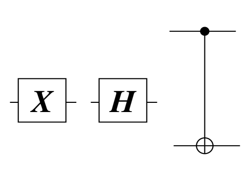
Figure 1.1: Diagrammatic Representations of $X$, $H$, and control-NOT respectively.

The effect of $X$ on computational basis is a logical NOT operation, $X|0\rangle=|1\rangle$ and $X|1\rangle=|0\rangle$. A Hadamard, $H$ transforms $|0\rangle$ into a uniform superposition of $|0\rangle$ and $|1\rangle$ i.e., $\frac{(|0\rangle+|1\rangle)}{\sqrt{2}}$ and $|1\rangle$ into $\frac{(|0\rangle-|1\rangle)}{\sqrt{2}}$. Applying $H$ for each of $n$ qubits initialized to $|0\rangle$, we can create a uniform superposition of $2^{n}$ computational bases, i.e., $\frac{1}{\sqrt{2^{n}}}\displaystyle\sum_{x=0}^{{2^{n}}-1}|x\rangle$. C-NOT takes two qubits as inputs and conditioned on the first qubit, it performs a logical NOT operation to the second qubit, e.g., $\mbox{C-NOT}|01\rangle=|01\rangle$ because the first qubit is $0$, and $\mbox{C-NOT}|11\rangle=|10\rangle$ because the first qubit is $1$. It is a unitary operation corresponding to a classical gate.

Recall that classically if we are given NOT and AND gates, we can construct a classical circuit for any boolean function. Such a set of gates is called a universal set of gates. Similarly, quantumly, we have universal sets of gates. This means that any unitary transformation on $n$ quantum bits maybe approximated to within a specified $\epsilon>1$ (in the spectral norm, say) by composing a sequence of these gates. One example involves the use of a C-NOT and a Hadamard with two additional one-qubit gates called a phase gate $S$, and $\pi/8$ gate $T$.

$$S=\left(\begin{array}[]{cc}1&0\\ 0&i\\ \end{array}\right),T=\left(\begin{array}[]{cc}1&0\\ 0&e^{i\pi/4}\\ \end{array}\right)$$

For the proof of the universality of this gate set, refer Section 4.5 in [NC00].

1.2.4 Quantum Algorithms and the Circuit Model

A quantum algorithm consists of quantum registers that hold qubits, and a series of unitary operations described by a quantum circuit. The registers are initialized to $|0\rangle$ except for the input register which is initialized to the bits of the problem instance, as in a classical circuit. The circuit consists of a sequence of gates from a universal set of quantum gates with the labels of the qubits the gates are applied to. In Figure 1.2, the registers are represented by black lines. As we apply operators we move from the left to the right of the circuit. At the end of the algorithm, i.e., at the right end of the circuit, a measurement is performed on one or more qubits in the computational basis, which gives an outcome of the algorithm. An algorithm is said to compute a boolean function with bounded error if when the input string $x$ is in the language, the algorithm accepts $x$ (has outcome $1$) with probability more than $3/4$, and when $x$ is not in the language, the algorithm accepts (i.e., has outcome $0$) with probability less than $1/4$.

For example, suppose we want to implement an algorithm that flips the phase if the registers both contain $|0\rangle$, but not otherwise. Then Figure 1.2 performs such algorithm. It first applies an $X$ gate to each register, and then applies a Hadamard gate to the second qubit, followed by a C-NOT conditioned on the first qubit, followed by a Hadamard on the second qubit, and finally applies $X$ gates to two of the qubits. This operator can be written as

$$I-2|00\rangle\langle 00|.$$

It is straightforward to check that both the circuit and the above matrix flips the phase of the qubit if they are both $0$.

The quantum time complexity of a (boolean) function is measured by the least number of gates required to implement an algorithm that computes the function with bounded error in terms of the size of the input. In Figure 1.2, the input size is two and the number of gates is seven.

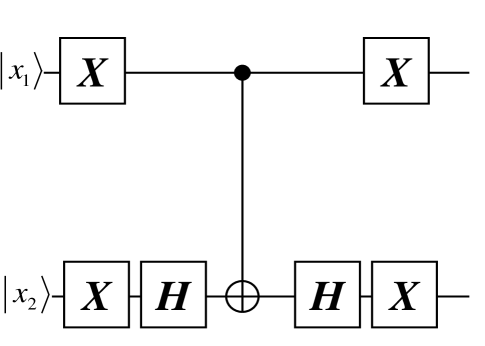
Figure 1.2: A Circuit that Implements a Phase Flip

1.2.5 Query Model and Quantum Query Complexity

We first formally define an oracle in terms of an operator.

Definition 2 (Oracle)

[NC00] An oracle $O$ for a function $f:\{1,\ldots,n\}\rightarrow\{0,1\}$ is a unitary operator that acts on a computational basis such that

$$O|x\rangle|q\rangle=|x\rangle|q\oplus f(x)\rangle,$$

where $|q\rangle$ is an oracle qubit with $q\in\{0,1\}$, which is flipped conditioned on $x\in\{1,\ldots,n\}$, i.e., flipped if $f(x)=1$. An oracle for a function with a larger range, $\{1,\ldots,n\}$ is defined similarly, with $O(\log n)$ qubits each for the query and the function value and $\oplus$ representing a bit-wise XOR.

Using an oracle, we can perform a query algorithm,

Definition 3 ($T$-Query Quantum Algorithm)

[BBC⁺01a] A $T$-query quantum algorithm $A$ with an oracle $O$ for function $f$ is defined as

$$A=U_{T}OU_{T-1}\ldots OU_{1}OU_{0},$$

where all the transformation are defined on a three register quantum memory consisting of the query register, the oracle response register and workplace qubits for the algorithms. The $U_{i}$’s are unitary transformations independent of the function $f$, and the algorithm only depends on the function $f$ through $T$ applications of $O$.

The query complexity of an algorithm is measured by the number of oracle operators we apply. The query complexity of computing a property $P$ of the oracle function $f$ is given by the least query complexity algorithm that computes $P(f)$.

For a search algorithm where an oracle outputs $f(x)=1$ if $x$ is a target of the search and the property being if a given set contains a target element, we usually prepare an oracle qubit as $\frac{|0\rangle-|1\rangle}{\sqrt{2}}$, so that we get

$$O\frac{1}{\sqrt{2^{n}}}\displaystyle\sum_{x=0}^{2^{n}-1}|x\rangle\left(\frac{|0\rangle-|1\rangle}{\sqrt{2}}\right)\rightarrow(-1)^{f(x)}\frac{1}{\sqrt{2^{n}}}\displaystyle\sum_{x=0}^{2^{n}-1}|x\rangle\left(\frac{|0\rangle-|1\rangle}{\sqrt{2}}\right).$$

Since the oracle qubit does not change throughout the algorithm, we could simply think of this oracle as flipping a phase if $f(x)=1$.

What would be the action of $O$ in a search algorithm? Suppose we have an initial state

$$|\psi\rangle=\frac{1}{\sqrt{2^{n}}}\displaystyle\sum_{x=0}^{2^{n}-1}|x\rangle,$$

and that $|\psi\rangle$ is a combination of two vectors, $|\alpha\rangle$ and $|\beta\rangle$, where the former is a uniform superposition of elements $x$ such that $f(x)=0$, and the latter contains the rest of elements. Then the act of applying the oracle is a reflection about the axis $|\alpha\rangle$ because

$$O(a|\alpha\rangle+b|\beta\rangle)=a|\alpha\rangle-b|\beta\rangle.$$

Recall the phase flip operator from the last section, which up to an overall sign of $-1$ is a reflection operator. Thus we can create the following reflection operator by removing $X$ gates in Figure 1.2.

$$2|0\rangle\langle 0|-I.$$

This construction extends in a straightforward manner to $n$ qubits. In general, in order to implement a phase flip on qubits that represent $n$, $O(\log{n})$ gates are required.

We can create another reflection operator also called Grover diffusion operator that reflects the state with the axis $|\psi\rangle$ by

$$H^{\oplus n}(2|0\rangle\langle 0|-I)H^{\oplus n}=2|\psi\rangle\langle\psi|-I.$$

Hence so far we have two reflection operators, $O$ and $2|\psi\rangle\langle\psi|-I$.

Lemma 4

Applying

$$G=\left(2|\psi\rangle\langle\psi|-I\right)O$$

is a rotation in a two-dimensional space spanned by $|\alpha\rangle$ and $|\beta\rangle$ by $2\theta$, where $\theta$ is the initial angle between $|\psi\rangle$ and $|\alpha\rangle$.

Lemma 4 also holds for the composition of reflections of any two vectors. We will use this fact later in this essay. In Figure 1.3, the action of $G$ is described geometrically. It first reflects $|\psi\rangle$ about the axis $|\alpha\rangle$, and then $O|\psi\rangle$ is reflected against the original state $|\psi\rangle$.

Figure 1.3: A Product of Two Reflections is a Rotation

In this one step of $G$, there is only one query $O$. In Grover’s algorithm, this process is repeated $O(\sqrt{N})$ times for $N=2^{n}$ so as to rotate the state of the query register close to $|\beta\rangle$: in the worst case when there is only one $x$ such that $f(x)=1$, $\theta\approx\frac{1}{\sqrt{n}}$. This gives a query complexity of $O(\sqrt{n})$.

1.2.6 Reducing Error Probability

In many quantum algorithms, we encounter a problem of reducing the error probability from a constant such as $1/4$ to polynomial close to $0$. An algorithm is said to compute a function $f$ with one-sided error given an input $x$ if the following two conditions hold,

1. If $x$ is not in the language, it rejects with probability $1$.

2. if $x$ is in the language, it accepts with probability at least $\epsilon>0$.

This means that we have a probability $(1-\epsilon)$ of having a false negative. In order to reduce the error probability to at most $1/2$, we repeat this algorithm for $k=\lceil-\frac{1}{\log{(1-\epsilon)}}\rceil\approx\frac{1}{\epsilon}$ times, because

$$(1-\epsilon)^{-\frac{1}{\log{(1-\epsilon)}}}\leq\frac{1}{2}.$$

During any one time in the $k$ repetition of the algorithms, if the algorithm accepts $x$, we terminate and decide “yes”. Most of the algorithms in this essay have one-sided error. For example, in element distinctness, if we find two different indices $i$ and $j$ such that $x_{i}\neq x_{j}$, we are sure it is in fact true.

In our algorithms, we will often compose bounded error quantum algorithms. In such cases, a quantum algorithm is used as a subroutine in place of an oracle. We would have to amplify, by repetition, the success probability of the subroutine so that the overall algorithm succeeds. This results in an additional factor of $O(\log T)$ in the query complexity where the complexity with an ideal oracle is $O(T)$. Such a scenario is studied in [HMdW03] as a quantum search with a bounded error oracle. The main result in [HMdW03] is that we only need to invoke the oracle $\sqrt{n}$ times as opposed to the obvious approach that gives $\sqrt{n}\log{n}$.

In this essay, whenever we have a one-sided error and we wish to amplify the success probability, we assume the procedure is modified as above. Moreover, if we have a case of imperfect oracle realized by a bounded error quantum algorithm, we apply the theorem in [HMdW03].

Chapter 2 Related Work

2.1 Quantum Walk of Szegedy

2.1.1 Element Distinctness

Recall from Chapter 1, the problem of Element Distinctness: given a function $f:[n]=\{1,2,\ldots,n\}\mapsto[m]$, $m\geq n$, as an oracle, we want to test if $f$ is one-one or not. If $f$ is not one-one, we say there is a collision. That is, $(i,j)$ collide if $f(i)=f(j)$, The function $f$ can also be written as a list of numbers: $f\equiv(f_{1},f_{2},\ldots,f_{n})$. The goal of the algorithm is to answer this question with as few queries to the oracle as possible.

The significance of this problem is that it is one of the applications of quantum walks that gives better bounds than classical counterparts. Underlying this quantum algorithm is a random walk. Ambainis was the first to adopt this classical walk into a quantum algorithm [Amb04b]. Classically, the straightforward algorithm to solve Element Distinctness is to go through the list one by one. Interestingly, this straightforward algorithm performs better than a random walk based algorithm classically which we will see in Section 2.1.2.

Fact 5

Classical query complexity of element distinctness is $\Theta(n)$.

Since it is optimal an unordered search may be reduced to element distinctness. However, in quantum scenario, quantum walk based algorithm performs better than the above bound. Quantum walk based algorithm is a quantum version of a random walk based algorithm, which is described below.

2.1.2 Classical Walk Based Algorithm

The following is a classical algorithm based on random walk for finding a collision.

Algorithm 1 A Classical Walk Algorithm for Element Distinctness

1:  Pick a uniformly random set $I$ of $r$ elements out of $[n]$ (call it an $r$-subset).

2:  Query $f$ at points in $I$.

3:  if There is a collision within $I$ then

4:     return  “Collision found” and elements that collide

5:  end if{Walk on $r$-subsets of $[n]$.} {(idea) Pick an element in the set and one not in the set uniformly at random (u.a.r.). Swap these elements. Note that we are maintaining the size of the subset.}

6:  for  $t\leq T$  do

7:     Pick $i\in I$ and $j\in[n]-I$ u.a.r.

8:     $I\leftarrow(I-\{i\})\cup\{j\}$.

9:     Query $f_{j}$.

10:     if There is a collision within $I$ then

11:        Output the elements that collide.

12:        return  

13:     end if

14:  end for

15:  print  “No collision” {i.e., $f$ is one-one.}

This walk is irreducible in the sense that there is a path between any pair of subsets. Let $\mathcal{T}$ be the first time the walk “hits” an $r$-subset containing a collision (hitting time).

Observation

$$Pr(\text{walk stops in two steps $|$ any state})\geq 1\cdot\frac{2}{n-r}\cdot\frac{r-1}{r}\cdot\frac{1}{n-r}.$$

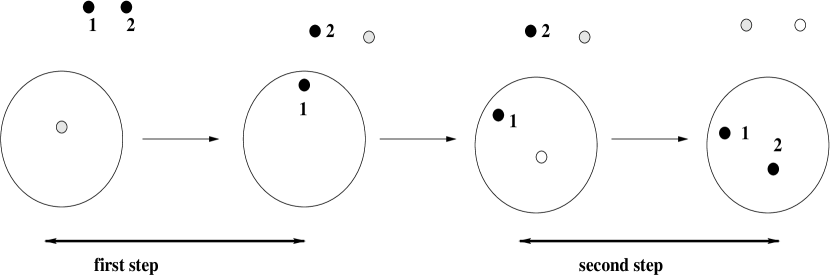
Figure 2.1: The Probability of the Walk Stopping in Two Steps

This is because in the worst case, there are exactly two elements that collide with each other, and initially, we do not have any element that form a colliding pair in the $r$-subset. Next we pick one of the two colliding elements from $n-r$ elements not in the set with probability $\frac{2}{n-r}$. In the second step, we first choose an element in the $r$-subset that is not part of the colliding set with probability $\frac{r-1}{r}$, and then we pick the other colliding element not in the $r$-subset with probability $\frac{1}{n-r}$ and swap these. In Figure 2.1, $1$ and $2$ are colliding elements not in the subset initially. It describes a sequence of transformation by which they are found by the algorithm. The hitting time for the walk is

$$E(\mathcal{T})\leq\frac{(n-r)^{2}r}{2(r-1)}.$$

There are more sophisticated arguments that give a better bound on $\mathcal{T}$. We will analyze hitting times more precisely.

2.1.3 Hitting Time in Classical Walks

Consider a Markov Chain on the state space $X$, ($|X|=N$) given by the transition matrix $P$, where $P=\left(p_{x,y}\right)$, $x,y\in X$ and

$$p_{x,y}=Pr(\text{making a transition to $y$ $|$ current state $=x$}).$$

This corresponds to general Markov Chains, in the sense that if we are at $x$, we move to any arbitrary state $y$ in the state space with probability $p_{x,y}$. $P$ is called a stochastic matrix, i.e., $\displaystyle\sum_{y}p_{x,y}=1$ for all $x$. So all the rows sum up to $1$.

We assume that the Markov Chain is

1. Symmetric: $p_{x,y}=p_{y,x}$. This makes the underlying graph of the walk undirected.

2. Irreducible: There is a path between every pair of states.

3. Aperiodic: There exists $x\in X$ and $t_{x}\geq 1$ such that

   $$Pr(\text{We reach $x$ in $t$ steps starting from $x$})>0$$

   for all $t\geq t_{x}$. Aperiodicity of the walk is equivalent to having an underlying graph that is not bipartite. This implies the same property for all $y\in X$ if the second property holds.

Figure 2.2: An Example of a Periodic Markov Chain

What are the properties of such Markov Chains?

1. Since $P$ is symmetric, it is equal to its transpose, $P=P^{\texttt{T}}$. So $P$ is doubly stochastic; both rows and columns sum up to $1$.

2. Let $s$ be any initial distribution, then $s^{\texttt{T}}P^{t}\longmapsto\pi^{\texttt{T}}=(\frac{1}{N},\frac{1}{N},\ldots,\frac{1}{N})$ as $t\rightarrow\infty$ in the $l_{1}$ metric. The distribution $\pi$ is called stationary distribution, which is a fixed point in a Markov Chain. So we have uniform stationary distribution.

3. $\pi^{\texttt{T}}P=\pi^{\texttt{T}}=(\frac{1}{N},\frac{1}{N},\ldots,\frac{1}{N})$: $\pi$ is an eigenvector of $P$ with eigenvalue of $1$. Since $P$ is symmetric, it is Hermitian, therefore it is diagonalizable and all the eigenvalues are real. Moreover, the other eigenvalues are strictly less than $1$: $\lambda_{1}=1>\lambda_{2}\geq\ldots\geq\lambda_{n}>-1$. The eigenvalue of $1$ is obtained from the irreducibility property. Aperiodicity implies all the eigenvalues are $>-1$.

In general, a marked state $M\subseteq X$ is a subset. For element distinctness, $M$ contains two colliding elements. Since we stop at a marked state, the transition matrix for this state is different from others. Suppose we would like to search for one of the marked states by simulating the walk and stopping when we see a state $x\in M$. The transition matrix now looks like

$$\tilde{P_{M}}=\left(\begin{array}[]{ccc}P_{M}&P^{\prime}\\ 0&I\\ \end{array}\right),$$ (2.1)

where $(P_{M}\;P^{\prime})$ are the rows of $P$ corresponding to $X-M$, $P_{M}$ is $P$ from which rows and columns corresponding to $M$ have been removed. The rows corresponding to the states in $M$ are $(0\;I)$ since once we reach $M$, we do not move to any other state.

What is the hitting time of $M$? Let $T$ be the hitting time for finding a marked state starting in distribution $s$.

Fact 6

$$E(T)=s_{M}^{\texttt{T}}(I-P_{M})^{-1}\cdot\mathbb{1},$$

where $s_{M}$ is the projection of $s$ onto $X-M$, and $\mathbb{1}^{\texttt{T}}=(1,1,\ldots,1)$. When $M$ is non-empty, and since the Markov Chain is ergodic all the eigenvalues of $P_{M}$ have absolute value less than $1$. Therefore the expression is well-defined.

Proof 2.1.7.

For any non-negative integer-valued random variable $T$, $E(T)=\displaystyle\sum_{t=0}^{\infty}Pr(T>t)$. In our case, $Pr(T>t)$ is the probability we have not reached the marked state after $t$ steps. This is also the probability that we are still in one of the states in $X-M$. Since the state distribution after $t$ steps is $s^{\texttt{T}}\tilde{P}^{t}$, where

$$\tilde{P}^{t}=\left(\begin{array}[]{ccc}P_{M}^{t}&P^{\prime}(t)\\ 0&I\\ \end{array}\right).$$

Let $\mathbb{1}_{X-M}$ denote a vector that contains $1$ for the first $|X-M|$ entries and $0$ for the rest. Then we have

$$Pr(\text{We are not in a marked state after $t$ steps})=s^{T}\tilde{P}^{t}1_{X-M}=s^{T}_{M}\tilde{P}^{t}_{M}\mathbb{1}.$$

Then,

$$\begin{array}[]{ll}E(T)&=\displaystyle\sum_{t=0}^{\infty}s_{M}^{T}P_{M}^{t}\mathbb{1}\\ \\ &=s_{M}^{T}(\displaystyle\sum_{t=0}^{\infty}P_{M}^{t})\mathbb{1}\\ \\ &=s_{M}^{T}(I-P_{M})^{-1}\mathbb{1}.\\ \end{array}$$

Stationary distribution for $P$ is a uniform distribution over all elements. Thus by judicially choosing initial state to be the stationary distribution, we get a good bound on hitting time.

Corollary 1.

a. If $s=(\frac{1}{N},\frac{1}{N},\ldots,\frac{1}{N})$, then hitting time $E(T)$ is

$$E(T)=\frac{1}{N}\cdot\mathbb{1}\cdot(I-P_{M})^{-1}\cdot\mathbb{1}.$$

b. Let $\mathbb{1}_{M}=\frac{(1,\ldots,1)}{\sqrt{N}}$. If the eigenvalues/vectors of $P_{M}$ are $(\lambda_{i},v_{i})$ and $\mathbb{1}_{M}=\displaystyle\sum_{i=1}^{N-m}\nu_{i}v_{i}$ then,

$$E(T)=\displaystyle\sum_{i=1}^{N-m}\nu_{i}^{2}(\frac{1}{1-\lambda_{i}}),$$ (2.2)

where $N$ is the normalization factor, $m=|M|$ is the size of marked subsets, and $\lambda_{i}$ is the $i$-th largest eigenvalue of $P_{M}$ in magnitude.

Note in the first part of Corollary 1, the eigenvalues of $(I-P_{M})^{-1}$ are $\frac{1}{1-\lambda_{i}}$, for each eigenvalue $\lambda_{i}$ of $P_{M}$. Also since we are working with real symmetric matrices, all the numbers $\nu_{i}$ are real.

The matrix $P_{M}$ is real, all the absolute values of eigenvalues of $P_{M}$ are strictly less than $1$, and along with the symmetry of $P_{M}$, it is orthogonally diagonalizable. This means we can choose ${v_{i}}$ such that they form an orthonormal set. Note that the spectral norm of a matrix is the largest singular value of the matrix. Since $P_{M}$ is symmetric, it is equivalent to the largest eigenvalue. Hence $\|P_{M}\|=\lambda_{1}$. Since $\displaystyle\sum\nu_{i}^{2}$ is at most $1$, we have, $E(T)\leq\frac{1}{1-\lambda_{1}}=\frac{1}{1-\|P_{M}\|}$.

In order to bound the hitting time, then we need to bound the largest eigenvalue of $P_{M}$.

Lemma 2.1.8 ([Sze04b]).

If the spectral gap($=1-\lambda_{2}(P)$) of $P$ is $\geq\delta$, and if $\frac{|M|}{|X|}\geq\epsilon$, then $\|P_{M}\|\leq 1-\frac{\delta\epsilon}{2}$.

In the above lemma, we define $\lambda_{i}(P)$ to be $i$-th largest eigenvalue of $P$ in magnitude. Note that since $P$ has a uniform distribution, $\lambda_{1}=1$. So the spectral gap, which is formally, the difference between the largest and the second largest eigenvalues in magnitude, is $\lambda_{1}(P)-\lambda_{2}(P)=1-\lambda_{2}(P)$.

Figure 2.3: $P_{ij}$ Moves from One State to Another With a Symmetric Difference of Two

To bound the hitting time of the walk , we would like an explicit formula for the spectral gap of $P$ to compute the upper bound of the spectra for $P_{M}$. Recall the state space of the walk is $X=\{\text{$r$-subsets of }[n]\}$. Given an $r$-subset, there are $r(n-r)$ other $r$-subsets to transition to by swapping one of the $r$ elements in the current subset with one of the $n-r$ elements not in the subset. Each of these $r(n-r)$ subsets have equal probability of being moved to from the current $r$-subset. Then

$$N=|X|={n\choose r},$$

and

$$\begin{array}[]{ll}p_{i,j}&=\left\{\begin{array}[]{cc}\frac{1}{r(n-r)}&\textrm{ if $|i\cap j|=r-1$}\\ 0\\ \end{array}\right.\\ &=\frac{J_{n,r,r-1}}{r(n-r)},\end{array}$$

where $J_{n,r,r-1}$ is a boolean matrix with entry $1$ iff $i$ and $j$ are subsets of size $r$, whose intersection is of size $r-1$.

Theorem 2.1.9 ([Knu91]).

There are $r+1$ eigenspaces of $J_{n,r,r-1}$, eigenvalues corresponding to

$$\lambda_{j}=(r-j)(n-r)-j(r-j+1),\;0\leq j\leq r.$$

We have $r\leq\frac{n}{2}$, otherwise we have a high probability of solving the problem in Line 3 in Algorithm 1. Also, $\lambda_{j}$ is a decreasing function of $j$. The eigenvalues are not all positive, e.g., for $j=r$, we have $\lambda_{r}=-r$. However, we are only interested in the first and the second largest eigenvalues, which are, $\lambda_{0}=r(n-r)$ and $\lambda_{1}=r(n-r)-n$. Since these are eigenvalues for $J_{n,r,r-1}$ and $P=\frac{J_{n,r,r-1}}{r(n-r)}$, the second largest eigenvalue for $P$ is $\frac{r(n-r)-n}{r(n-r)}$. From these, we can compute the spectral gap: $1-\frac{\lambda_{1}}{r(n-r)}=\frac{n}{r(n-r)}>\frac{1}{r}$. Remembering that $M$ is the set of $r$-subsets that contain a colliding pair of elements, in order to lower bound the fraction of marked elements, we need to consider the worst case scenario where we have exactly one pair of colliding elements.

$$\frac{|M|}{|X|}\geq\frac{{n\choose r-2}}{{n\choose r}}=\frac{r(r-1)}{(n-r-2)(n-r-1)}\geq\frac{r^{2}}{2n^{2}}$$

for $r=o(n)$ when approximation involved.

From this, we have

$$\begin{array}[]{ll}\|P_{M}\|&\leq 1-\frac{\frac{r^{2}}{2n^{2}}\frac{1}{r}}{2}\\ &=1-\frac{r}{4n^{2}}.\\ \end{array}$$

So

$$E(T)\leq\frac{1}{1-\|P_{m}\|}\leq\frac{4n^{2}}{r}=O\left(\frac{n^{2}}{r}\right).$$

This is a bound on the hitting time of the algorithm. The query complexity of the algorithm is calculated as follows. We need to make $r$ initial queries for the values of each element in the initial $r$-subset. At each of the $O(\frac{n^{2}}{r})$ iteration of the walk, we need to query the value of the new element we swapped into the subset. Thus, we have $O(r+\frac{n^{2}}{r})$ query complexity. This is minimized when $r=n$ and gives $O(n)$ query complexity. This is equivalent to checking every element in the entire set, thus giving no speedup to the straightforward algorithm of sequentially checking every element in the set.

Now we are interested in the quantization of the classical algorithm we have discussed thus far.

2.1.4 Quantization of the classical walk

Figure 2.4: A Bipartite Walk

The first quantization of random walk in Algorithm 1 was proposed by Ambainis [Amb04b], which is described in Section 2.2. A new kind of quantization of classical walks was proposed by Szegedy [Sze04b], which we present here in detail. The walk is over a bipartite graph. Each side of the graph contains $r$-subsets as vertices. A pair of vertices in the left and the right hand side of the graph are connected only if one can be changed into another on the opposite side by removing one of the elements in the subset and adding one that is not in the current set. This is equivalent to having two vertices connected if they differ in exactly two elements. The probability of moving from a subset $x$ in the left side of the graph to a subset $y$ in the right side of the graph is given by $p_{x,y}$. For each side of the graph, we create a state,

$$|\phi_{x}\rangle=\displaystyle\sum_{y}\sqrt{p_{x,y}}|x\rangle|y\rangle$$

for the transition from $x$ on the left side to all of its neighbors $y$ on the right side of the graph, and

$$|\psi_{y}\rangle=\displaystyle\sum_{x}\sqrt{p_{x,y}}|x\rangle|y\rangle$$

similarly. Note that,

a. $\{\phi_{x}\}_{x}$ and $\{\psi_{y}\}_{y}$ are orthonormal sets because each $|x\rangle$ and $|y\rangle$ are distinct.

b. Let $E_{1}=span\{\phi_{x}\}_{x}$ and $E_{2}=span\{\psi_{y}\}_{y}$ and $\pi_{1}$, $\pi_{2}$ to be orthonormal projections onto $E_{1}$, $E_{2}$ respectively. We define two unitary operators $R_{1}$ and $R_{2}$ as $R_{1}=2\Pi_{1}-I$ and $R_{2}=2\Pi_{2}-I$.

Then $R_{1}$ is unitary because it can be implemented using the combination of unitary gates similar to the reflection operator in Section 1.2.4. We can see that $R_{1}$ is actually a reflection operator about the space $E_{1}$ because

$$\begin{array}[]{ll}R_{1}|\varphi\rangle&=(2\pi_{1}-I)|\varphi\rangle\\ &=(2\displaystyle\sum_{x}|\phi_{x}\rangle\langle\phi_{x}|-I)|\varphi\rangle\\ &=\displaystyle\sum_{x}(2|\phi_{x}\rangle\langle\phi_{x}|-I)|\varphi\rangle\\ &=\left\{\begin{array}[]{cc}|\varphi\rangle&\text{if $\varphi\in E_{1}$}\\ -|\varphi\rangle&\text{if $\varphi\in E_{1}^{\bot}$}\\ \end{array}\right.\\ \end{array}$$

Similarly $R_{2}$ is unitary and is a reflection about the space $E_{2}$.

Definition 2 (Quantitization of a M.C. $P$).

$$W_{P}=R_{2}R_{1}$$

Why is this a natural definition? The straightforward way to define a step of the walk is

$$\begin{array}[]{ll}|x\rangle|\overline{0}\rangle&\rightarrow|x\rangle\displaystyle\displaystyle\sum_{y}\sqrt{p_{x,y}}|y\rangle\\ &\rightarrow|x\displaystyle\rangle\displaystyle\sum_{y}\sqrt{p_{x,y}}|y\rangle\displaystyle\displaystyle\sum_{z}\sqrt{p_{y,z}}|z\rangle\\ &\rightarrow|x\rangle\displaystyle\displaystyle\sum_{y}\sqrt{p_{x,y}}|y\rangle\displaystyle\displaystyle\sum_{z}\sqrt{p_{y,z}}|z\rangle\displaystyle\displaystyle\sum_{a}\sqrt{p_{z,a}}|a\rangle\\ \end{array}$$

But this is just a simulation of a classical walk. Instead, we keep the memory of the previous step only. To do so, we need an operator that diffuses $x$ into all the neighbors $y$ and vice versa.

Another way to see that the definition of the quantized walk is natural is to look at the Grover diffusion operator as an operator to move from a vertex in a complete graph to one of the adjacent vertices with equal probability. This idea was introduced in [Wat01]. Algorithm 2 describes Szegedy’s algorithm.

Algorithm 2 Szegedy’s Quantization of a Random Walk

1:  Let $|\phi_{0}\rangle=\frac{1}{\sqrt{N}}\displaystyle\sum_{x}|\phi_{x}\rangle=\frac{1}{\sqrt{N}}\displaystyle\sum_{x,y}\sqrt{p_{x,y}}|x\rangle|y\rangle=\frac{1}{\sqrt{N}}\displaystyle\sum_{y}|\phi_{y}\rangle$

2:  Measure if the first register is marked or not.

3:  if The first register is marked then

4:     return  ‘‘Found marked element.’’

5:  end if

6:  Apply $H\otimes I$ to $|0\rangle|\phi_{01}\rangle$ to get $\frac{1}{\sqrt{2}}(|0\rangle|\phi_{01}\rangle+|1\rangle|\phi_{01}\rangle)$

7:  Pick $t$ u.a.r. from $[0,\ldots,T]$

8:  for $i\leq T$ do

9:     Apply controlled-$W_{\tilde{P}}$ conditioned on the first register. {The modified matrix $\tilde{P}$ in Equation 2.1 lets us remain in the same state once we arrive at the marked state.}

10:  end for{ Now we have $\frac{1}{\sqrt{2}}(|0\rangle|\phi_{01}\rangle+|1\rangle W_{\tilde{P}}^{t}|\phi_{01}\rangle)$}

11:  Apply $H\otimes I$ to get $\frac{1}{2}|0\rangle(|\phi_{01}\rangle+W_{\tilde{P}}^{t}|\phi_{01}\rangle)+\frac{1}{2}|1\rangle(|\phi_{01}\rangle-W_{\tilde{P}}^{t}|\phi_{01}\rangle)$

12:  Measure the first register.

13:  if There is a ’1’ in the first register then

14:     return  ‘‘Detected marked element.’’

15:  else

16:     return  ‘‘No marked element.’’

17:  end if

Szegedy defines the quantum hitting time as follows.

Definition 3 ([Sze04a]).

$T$ is an $c$-deviation-on-average time with respect to $|\phi\rangle$ if

$$\frac{1}{T+1}\displaystyle\sum_{t=0}^{T}\|W_{p}^{t}|\phi\rangle-|\phi\rangle\|_{2}^{2}\geq c_{.}$$

This was defined so that after $T$ steps of the walk, the average deviation of the initial state is very high. That is, the state is significantly skewed towards the marked state and so the probability of observing the marked state is high. Since the walk is realized by unitary evolution it cannot end up in a marked state. Instead, it can cycle through states with high amplitude on marked states.

Next we compute the complexity of this algorithm. One step of the walk is $R_{1}$ followed by $R_{2}$. We show here that $R_{1}$ can be implemented efficiently. $R_{2}$ can be implemented similarly. Recall that

$$\begin{array}[]{ll}R_{1}&=(2\Pi_{1}-I)\\ &=\left(2\displaystyle\displaystyle\sum_{x}|\phi_{x}\rangle\langle\phi_{x}|-I\right)\\ &=\displaystyle\displaystyle\sum_{x}\left(2|\phi_{x}\rangle\langle\phi_{x}|-I_{x}\right),\\ \end{array}$$

where $I_{x}$ is identity on $|x\rangle\otimes\mathbb{C}^{x}$. The last line follows from the fact that we are working on

$$\begin{array}[]{ll}\mathbb{C}^{X\times X}&\cong\mathbb{C}^{X}\otimes\mathbb{C}^{X}\\ &\cong\bigoplus_{x}|x\rangle\otimes\mathbb{C}^{X},\\ \end{array}$$

so $R_{1}$ which acts on $\mathbb{C}^{X}\otimes\mathbb{C}^{X}$ can be decomposed into the direct sum of $|X|$ diffusion operators, $2|\phi_{x}\rangle\langle\phi_{x}|-I_{x}$. Since this is the reflection in $|x\rangle\otimes\mathbb{C}^{X}$ about $|\phi_{x}\rangle$, this can be written as

$$|x\rangle\langle x|\otimes\left(U_{x}(2|\overline{0}\rangle\langle\overline{0}|-I)U^{{\dagger}}_{x}\right),$$

and $2|\overline{0}\rangle\langle\overline{0}|-I$ can be implemented using $O(\log{|X|})$ gates similarly to the construction of a circuit for $2|00\rangle\langle 00|-I$ in Section 1.2.4.

From the above argument, we see that if there is an efficient procedure to implement the transformation

$$\left(I\otimes U_{x}\right)|x\rangle|\overline{0}\rangle=|x\rangle\displaystyle\sum_{y}\sqrt{p_{x,y}}|y\rangle,$$

then the algorithm can be implemented efficiently.

2.1.5 Hitting Time in Quantum Walks

In order to analyze the deviation time, it suffices to take a look at the eigenvalues and eigenvectors of one step of the walk. This is because for a unitary operator $U=\displaystyle\sum_{j}e^{i\theta_{j}}|v_{j}\rangle\langle v_{j}|$ with $\{|v_{j}\rangle\}$ being the orthonormal eigenvectors of $U$, $U^{t}=\displaystyle\sum_{j}e^{i\theta_{j}t}|v_{j}\rangle\langle v_{j}|$ so it has the same set of eigenvectors.

Recall that $W_{P}=R_{2}R_{1}=(2\Pi_{2}-I)(2\Pi_{1}-I)$, where $\Pi_{i}$ is an orthogonal projection to $E_{i}$, and $E_{1}$ is the space spanned by $|\phi_{x}\rangle$ and similarly for $E_{2}$. Let $A=\displaystyle\sum_{x}|\phi_{x}\rangle\langle x|$ and $B=\displaystyle\sum_{y}|\phi_{y}\rangle\langle y|$. Note that the dimension of the space in which $|\phi_{x}\rangle$ lies is $N^{2}$ and that of $\langle x|$ is $N$. Then we can write $W_{P}=R_{2}R_{1}$ as $(2AA^{{\dagger}}-I)(2BB^{{\dagger}}-I)$ because $\Pi_{1}=\displaystyle\sum_{x}|\phi_{x}\rangle\langle\phi_{x}|=AA^{{\dagger}}$, and similarly for $\Pi_{2}$. Note that $A$ and $B$ are norm-preserving operations because $A^{{\dagger}}A=I=B^{{\dagger}}B$ and $A$ maps a vector in $\mathbb{C}^{x}$ into its subspace $E_{1}$ and similarly for $B$.

Suppose a vector $v\in(E_{1}+E_{2})^{\bot}$. Then $v$ lies in the space orthogonal to both $E_{1}$ and $E_{2}$. Since $R_{i}$ reflects a vector orthogonal to $E_{i}$, then $v$ is reflected by both $R_{1}$ and $R_{2}$. Then applying a walk operator $W_{P}=R_{2}R_{1}$ does not change $v$. Hence $W_{P}|v\rangle=|v\rangle$, and the subspace spanned by such $v$’s is an invariant subspace, an eigenspace with eigenvalue $1$. Thus we only need to analyze the behavior of $W_{P}$ in $E_{1}+E_{2}$. Suppose we have $|w\rangle,|v\rangle\in\mathbb{C}^{X}$, then we want to analyze the action of $R_{2}$ on $A|w\rangle$ and the action of $R_{1}$ on $B|v\rangle$. (Since $A|w\rangle\in E_{1}$, the action of $R_{1}$ on $A|w\rangle$ is identity.) Since

$$\begin{array}[]{ll}R_{2}A|w\rangle&=2\Pi_{2}A|w\rangle-A|w\rangle\\ &=2B(B^{{\dagger}}A)|w\rangle-A|w\rangle,\\ \end{array}$$

where the first term of the last line lies in $E_{2}$ and the second term in $E_{1}$, and similarly,

$$R_{1}B|v\rangle=2A(A^{{\dagger}}B)|v\rangle-B|v\rangle,\\$$

we define the discriminant of $A$ and $B$ as follows.

Definition 4.

The discriminant matrix $D$ of $A$ and $B$ is $D=A^{{\dagger}}B$.

Theorem 5.

If $D=\displaystyle\sum_{j}\delta_{j}|w_{j}\rangle\langle v_{j}|$ is the singular value decomposition of $D$, then

a) $0\leq\delta_{j}\leq 1$.

b) The space generated by $\{Aw_{j},Bv_{j}\}$, for all $j$ where $(w_{j},v_{j})$ is a pair of singular vectors is invariant under $W_{P}$. And $W_{P}$ restricted to this space is a composition of a reflection about $Aw_{j}$ followed by a reflection about $Bv_{j}$.

Let the angle between $Aw_{j}$ and $Bv_{j}$ be $\theta_{j}$, that is the singular value corresponding to $Aw_{j}$ and $Bv_{j}$ be $\langle w_{j}|A^{{\dagger}}B|v_{j}\rangle=\langle w_{j}|D|v_{j}\rangle=\cos{\theta_{j}}$, for $\theta_{j}\in[0,\pi/2]$. Recall from Lemma 4 that a product of two reflections about two reflectors $|\phi\rangle$ and $|\psi\rangle$ is a rotation by an angle $2\theta$, where $\theta$ is an angle between the vectors $|\phi\rangle$ and $|\psi\rangle$. Similarly then $W_{P}$ is a rotation by $2\theta_{j}$ in this subspace.

Proof 2.1.10 (Theorem 5-a).

Singular values are taken to be real and non-negative by convention, so $\delta_{j}\geq 0$. Since $A$, $B$ are norm-preserving $\|Aw\|=\|w\|$ and $\|Bv\|=\|v\|$. Using these facts,

$$\begin{array}[]{ll}\delta_{j}&\leq\max_{\{|\alpha\rangle,|\beta\rangle\}}|\langle\beta|D|\alpha\rangle|\\ &=\max_{\{|\alpha\rangle,|\beta\rangle\}}|\langle\beta|A^{\dagger}B|\alpha\rangle|\\ &\leq\max_{\{|\alpha\rangle,|\beta\rangle\}}\|A|\beta\rangle\|\cdot\|B|\alpha\rangle\|\\ &\leq 1.\\ \end{array}$$

Hence $\delta_{j}\leq 1$.

Proof 2.1.11 (Theorem 5-b).

As we mentioned before, we only need to consider the action of $W_{P}$ on $Aw_{j}$ and $Bv_{j}$ and that $Aw_{j}$ is invariant by $R_{1}$ and $Bv_{j}$ is invariant by $R_{2}$.

$$\begin{array}[]{ll}W_{P}|Aw_{j}\rangle&=(2\Pi_{2}-I)A|w_{j}\rangle\\ &=(2(BB^{{\dagger}})-I)A|w_{j}\rangle\\ &=2B(B^{{\dagger}}A|w_{j}\rangle)-A|w_{j}\rangle\\ &=2BD^{{\dagger}}|w_{j}\rangle-A|w_{j}\rangle\\ &=2\delta_{j}B|v_{j}\rangle-A|w_{j}\rangle\\ &=(\cos{\theta_{j}}B|v_{j}\rangle)-(A|w_{j}\rangle-\cos{\theta_{j}}B|v_{j}\rangle).\\ \end{array}$$

The first term in the last line is the component of $A|w_{j}\rangle$ that is along $B|v_{j}\rangle$ and the second term is the component of $A|w_{j}\rangle$ that is orthogonal to $B|v_{j}\rangle$. So, on $A|w_{j}\rangle$, $R_{1}$ is a reflection about $A|w_{j}\rangle$ (identity in this case), and $R_{2}$ is a reflection about $B|v_{j}\rangle$ (because of the orthogonal component) in the subspace. Similarly, on $B|v_{j}\rangle$, $R_{1}$ is a reflection about $A|w_{j}\rangle$ (because of the orthogonal component), and $R_{2}$ is a reflection about $B|v_{j}\rangle$ (identity) in the subspace.

Using Theorem 5, we are ready to estimate the deviation time with the initial state,

$$\begin{array}[]{ll}|\phi_{01}\rangle&=\frac{1}{\sqrt{N}}\displaystyle\sum_{x\in X-M}|x\rangle\displaystyle\sum_{y\in X}\sqrt{p_{x,y}}|y\rangle\\ &=\frac{1}{\sqrt{N}}\displaystyle\sum_{x\in X-M}|\phi_{x}\rangle,\\ \end{array}$$

because $|\phi_{01}\rangle$ is the state that remains after the measurement in Step 3 of Algorithm 2. We would like to bound $T$ such that

$$\frac{1}{T+1}\displaystyle\sum_{t=0}^{T}\|W_{\tilde{P}}^{t}|\phi_{01}\rangle-|\phi_{01}\rangle\|^{2}\geq c(1-\epsilon)$$

for some small positive constant $c$ and $\epsilon$ being the fraction of marked elements. This is because by Szegedy’s definition in Definition 3, the hitting time is the time it takes for the state to be significantly different from the initial state, greatly skewed towards the marked state. That is, we want the $L_{2}$ norm of the difference between the final and the initial state to be at least as large as the fraction of unmarked elements. This ensures that when we measure the final state, we detect a large deviation from the initial state. The term in the summation is $2(1-\epsilon-\langle\phi_{01}|W_{\tilde{P}}^{t}|\phi_{01}\rangle)$ because $|\phi_{01}\rangle=\displaystyle\sum_{x\in X-M}\frac{1}{\sqrt{N}}|\phi_{x}\rangle$ and so $\||\phi_{01}\rangle\|^{2}=1-\epsilon$, so we need to upper bound $\frac{1}{T+1}\displaystyle\sum_{t=0}^{T}\langle\phi_{01}|W_{\tilde{P}}^{t}|\phi_{01}\rangle$.

Now

$$\begin{array}[]{ll}D(x,y)&=\langle x|D|y\rangle\\ &=\langle x|A^{{\dagger}}B|y\rangle\\ &=\langle x|\left(\displaystyle\sum_{z}|z\rangle\langle\phi_{z}|\right)\left(\displaystyle\sum_{u}|\phi_{u}\rangle\langle u|\right)|y\rangle\\ &=\langle\phi_{x}|\phi_{y}\rangle\\ &=\langle x|\left(\displaystyle\sum_{y}\sqrt{p_{x,y}}\langle y|\right)\left(\displaystyle\sum_{x}\sqrt{p_{y,x}}|x\rangle\right)|y\rangle\\ &=\sqrt{p_{x,y}}\sqrt{p_{y,x}},\\ \end{array}$$

then for $D_{\tilde{P}}$, the $(x,y)$ entry is $\sqrt{\tilde{p}_{x,y}}\sqrt{\tilde{p}_{y,x}}$. Since if exactly one of $x$ or $y$ is marked, $\sqrt{\tilde{p}_{x,y}}$ or $\sqrt{\tilde{p}_{y,x}}$ is $0$, the entry of $D_{\tilde{P}}$ is zero if exactly one of $x$ or $y$ is marked. Also since $P_{M}$, and $I$ are symmetric, for $(x,y)$ both being unmarked or marked, we have $P_{M}$ or $I$ respectively as diagonal blocks in $D_{\tilde{P}}$. So

$$D_{\tilde{P}}=\left(\begin{array}[]{cc}P_{M}&0\\ 0&I\\ \end{array}\right).$$

Now we are ready to use Theorem 5. Let the normalized eigenvectors of $P_{M}$ be $\{v^{\prime}_{k}\}_{k}$ with eigenvalues $\lambda_{k}$, and denote $v_{k}$ for $v^{\prime}_{k}$ padded with $0$ to make an eigenvector of $D_{\tilde{P}}$. Since $P_{M}$ is symmetric, all the eigenvectors are orthogonal. The rest of the eigenvectors of $D_{\tilde{P}}$ are $\{|x\rangle\}_{x}$ for $x\in M$. These vectors are also orthogonal to each other, and all $n$ eigenvectors of $D_{\tilde{P}}$ are orthogonal to each other as well. So its eigenvectors are the singular vectors and the absolute value of the eigenvalues give the singular values because some eigenvalues may be negative. Then from Theorem 5, the invariant subspaces of $W_{\tilde{P}}$ are the subspaces $F_{k}$ spanned by the pairs $(Av_{k},Bv_{k})$ with singular value $|\lambda_{k}|$ for all $k$ and the subspaces $F_{x}$ spanned by the pairs $(A|x\rangle,B|x\rangle)$ with singular values $1$ for all $x\in M$. Since the product of two reflections is a rotation as we have seen before, the action of $W_{\tilde{P}}$ is a rotation of the subspace $F_{k}$ by $2\theta_{k}$, where $\theta_{k}$ is the angle between $Av_{k}$ and $Bv_{k}$:

$$\langle v_{k}|A^{\dagger}B|v_{k}\rangle=\cos{\theta_{k}},$$

This is also equal to the singular value of $A^{\dagger}B=D$ corresponding to $v_{k}$, $\theta_{k}=\cos^{-1}{|\lambda_{k}|}$. Also $\theta_{k}\in(0,\pi/2]$ cannot be zero because $\cos{\theta_{k}}=|\lambda_{k}|<1$ and from Theorem 2.1.8, $\|P_{M}\|=\lambda_{1}=1-\frac{\delta\epsilon}{2}<1$ assuming that $\epsilon\neq 0$. So $W_{\tilde{P}}^{t}$ rotates the subspaces by $2\theta_{k}t$.

Observation
a)

$$|\phi_{01}\rangle\in span\{Av_{k}\}_{k}$$

because

$$\begin{array}[]{ll}|\phi_{01}\rangle&=\frac{1}{\sqrt{N}}\displaystyle\sum_{x\in X-M}|\phi_{x}\rangle\\ &=\frac{1}{\sqrt{N}}\displaystyle\sum_{x\in X-M}\left(\displaystyle\sum_{z}|\phi_{z}\rangle\langle z|\right)|x\rangle\\ &=\frac{1}{\sqrt{N}}\displaystyle\sum_{x\in X-M}A|x\rangle\\ \end{array}$$

and $|x\rangle\in span_{k}\{v_{k}\}$ for $n\in X-M$. So $|\phi_{01}\rangle$ is spanned by $Av_{k}$ for all $k$.

b)

$$\||\phi_{01}\rangle\|^{2}=1-\epsilon$$

because

$$\begin{array}[]{ll}\||\phi_{01}\rangle\|^{2}&=\frac{1}{N}\displaystyle\sum_{x\in X-M}\langle\phi_{x}|\phi_{x}\rangle\\ &=\frac{|X-M|}{N}\\ &=1-\epsilon.\\ \end{array}$$

So we normalize the initial state and also write this as the linear combination of the spanning set,

$$\frac{|\phi_{01}\rangle}{\sqrt{1-\epsilon}}=\displaystyle\sum_{k}\nu_{k}A|v_{k}\rangle.$$ (2.3)

Note that the square of the amplitudes sum up to $1$ so $\displaystyle\sum_{k}\nu_{k}^{2}=1$. Let $|z_{k}\rangle=A|v_{k}\rangle$. Then $|z_{k}\rangle$ are orthonormal to each other because $|v_{k}\rangle$ are orthonormal to each other. $A$ preserves inner products:

$$\begin{array}[]{ll}\langle z_{k}|z_{k^{\prime}}\rangle&=A^{\dagger}A\langle v_{k}|v_{k^{\prime}}\rangle\\ &=\langle v_{k}|A^{\dagger}A|v_{k^{\prime}}\rangle\\ &=\langle v_{k}|v_{k^{\prime}}\rangle\\ &=0.\\ \end{array}$$

Claim 6.

If $T\geq 100\displaystyle\sum_{k}\frac{\nu_{k}^{2}}{\theta_{k}}$,

$$\begin{array}[]{ll}\frac{1}{T+1}\displaystyle\sum_{t=0}^{T}\|W_{\tilde{P}}^{t}|\phi_{01}\rangle-|\phi_{01}\rangle\|^{2}&=2\left((1-\epsilon)-\frac{1}{T+1}\displaystyle\sum_{t=0}^{T}\langle\phi_{01}|W_{\tilde{P}}^{t}|\phi_{01}\rangle\right)\\ &\geq c(1-\epsilon),\end{array}$$

for some constant $2\geq c>0$.

This means

$$\frac{1}{T+1}\displaystyle\sum_{t=0}^{T}\langle\phi_{01}|W_{\tilde{P}}^{t}|\phi_{01}\rangle<\left(1-\frac{c}{2}\right)\left(1-\epsilon\right).$$

Proof 2.1.12.

From Equation 2.3

$$\begin{array}[]{ll}\langle\phi_{01}|W_{\tilde{P}}^{t}|\phi_{01}\rangle&=\frac{1}{1-\epsilon}\displaystyle\sum_{k_{1},k_{2}}\nu_{k_{1}}\nu_{k_{2}}\langle z_{k_{1}}|W_{\tilde{P}}^{t}|z_{k_{2}}\rangle\\ &=\frac{1}{1-\epsilon}\displaystyle\sum_{k}\nu_{k}^{2}\langle z_{k}|W_{\tilde{P}}^{t}|z_{k}\rangle\\ &=\frac{1}{1-\epsilon}\displaystyle\sum_{k}\nu_{k}^{2}\cos{(2\theta_{k}t)},\\ \end{array}$$

because $|z_{k}\rangle$’s are orthonormal to each other and belong to orthogonal eigenspaces of $W_{\tilde{P}}$. The last line is obtained from the fact that the angle between $|z_{k}\rangle$ and $W_{\tilde{P}}^{t}|z_{k}\rangle$ is $2\theta_{k}t$ since one step of $W_{\tilde{P}}$ rotates the subspace by $2\theta_{k}$, and so $\langle z_{k}|W_{\tilde{P}}^{t}|z_{k}\rangle=\cos{(2\theta_{k}t)}$.

Now we use three mathematical identities to bound $\displaystyle\sum_{t=0}^{T}\cos{(2\theta_{k}t)}$. First,

$$\cos{(\omega t)}=\frac{e^{i\omega t}+e^{-i\omega t}}{2}.$$

So the sum of cosines is a sum of two geometric series. Using the formula for the sum of geometric series we have,

$$\begin{array}[]{ll}\frac{1}{T+1}\displaystyle\sum_{t=0}^{T}\langle\phi_{01}|W_{\tilde{P}}^{t}|\phi_{01}\rangle&\leq(1-\epsilon)\displaystyle\sum_{k}\nu_{k}^{2}\frac{1}{T+1}\frac{\cos{(2\theta_{k}T)}-\cos{(2\theta_{k}(T+1))}+1-\cos{(2\theta_{k})}}{2(1-\cos{(2\theta_{k}}))}.\\ \end{array}$$

Next, we use

$$|\cos{\alpha}-\cos{\beta}|\leq|\alpha-\beta|$$

to bound the numerator and use

$$\cos{\alpha}\leq 1-\frac{\alpha^{2}}{8}\text{ for $\alpha\in[-3.79,3.79]$},$$

to bound the denominator. Note that here, $\alpha=2\theta_{k}$ and $\theta_{k}\in(0,\frac{\pi}{2}]$ as mentioned before, so the third inequality can be applied.

Using these, we get

$$\begin{array}[]{ll}\frac{1}{T+1}\displaystyle\sum_{t=0}^{T}\langle\phi_{01}|W_{\tilde{P}}^{t}|\phi_{01}\rangle&\leq(1-\epsilon)\frac{1}{T+1}\displaystyle\sum_{k}\nu_{k}^{2}\frac{2\theta_{k}+2\theta_{k}}{2((2\theta_{k})^{2})/8}\\ &=(1-\epsilon)\frac{4}{T+1}\displaystyle\sum_{k}\frac{\nu_{k}^{2}}{\theta_{k}}\\ &\leq(1-\epsilon)\frac{4}{100}.\\ \end{array}$$

The last line comes from the fact that we have chosen $T\geq 100\displaystyle\sum_{k}\frac{v_{k}^{2}}{\theta_{k}}$. So the claim holds for $\left(1-\frac{c}{2}\right)=\frac{1}{25}$ or $c=\frac{48}{25}$.

We can relate the hitting time of the walk with the eigenvalues of $P_{M}$.

Corollary 7.

$c$-deviation on average time for $W_{\tilde{P}}$ with respect to $\frac{|\phi_{01}\rangle}{\sqrt{1-\epsilon}}$ is $O\left(\frac{1}{\sqrt{1-\|P_{M}\|}}\right)$.

Proof 2.1.13.

We know that $T\geq 100\displaystyle\sum_{k}\frac{\nu_{k}^{2}}{\theta_{k}}$ and that $\cos{\theta_{k}}=|\lambda_{k}|$. Then

$$\begin{array}[]{ll}\theta_{k}\geq\sin{\theta_{k}}&=\sqrt{1-\cos^{2}{\theta_{k}}}\\ &=\sqrt{1-\lambda_{k}^{2}}\\ &\geq\sqrt{1-\lambda_{k}},\\ \end{array}$$

because $\lambda_{k}\leq 1$.

So,

$$T\leq 100\displaystyle\sum_{k}\frac{\nu_{k}^{2}}{\sqrt{1-\lambda_{k}^{2}}}\leq\frac{100}{\sqrt{1-\|P_{M}\|}}\displaystyle\sum_{k}\nu_{k}^{2}$$

because $\displaystyle\sum_{k}\nu_{k}^{2}=1$ and any eigenvalue in $P_{M}$ is at most the largest eigenvalue of $P_{M}$ which is $\|P_{M}\|$. This means that the hitting time $T\in O\left(\frac{1}{\sqrt{1-\|P_{M}\|}}\right)$.

Recall that the classical hitting time for a symmetric transition matrix is $O\left(\frac{1}{1-\|P_{M}\|}\right)$, so using Szegedy’s walk we have quadratic speedup.

Theorem 2.1.14 ([Sze04a]).

For the quantum walk based on a transition matrix $P$ with eigenvalue gap of $\delta$, the fraction of marked elements $|M|/|X|$ at least $\epsilon$, in time $O\left(1/\sqrt{\delta\epsilon}\right)$, Algorithm 2 detects a marked element with probability at least $\frac{1}{1000}$ if it exists, in $O(1/\sqrt{\delta\epsilon})$ application of $W_{\tilde{P}}$.

Proof 2.1.15.

If a marked element exists, either a marked element is detected in Step 2 with probability $\epsilon$, or a deviation is detected in Step 11 with probability $\geq\frac{1}{4(T+1)}\displaystyle\sum_{t=0}^{T}\|W_{\tilde{P}}^{t}|\phi_{01}\rangle-|\phi_{01}\rangle\|^{2}\geq\frac{12}{25}(1-\epsilon)$. Then the net probability of success is $\epsilon+\frac{12}{25}(1-\epsilon)\geq\frac{12}{25}+\frac{13\epsilon}{25}$. Here, $T=O(\frac{1}{\sqrt{1-\|P_{M}\|}})$ from Corrollary 7 and Lemma 2.1.8.

The consequence of Theorem 2.1.14 is that it suffices to analyze the classical version of the walk in order to bound the quantum hitting time. Suppose we have three different costs, time or query, associated with a classical walk based algorithm. A setup cost, $s(r)$, an update cost $u(r)$ and a checking cost $c(r)$. A setup cost is the cost required to set up the initial $r$-subset, an update cost is the cost to maintain the data pertaining to the $r$-subset during the walk, and a checking cost is the cost needed to see if we have a marked subset. Then the total quantum complexity of this algorithm is

$$s(r)+\frac{1}{\sqrt{\delta\epsilon}}\left(u(r)+c(r)\right).$$ (2.4)

Throughout the rest of the essay, we will describe the classical versions of the algorithms to obtain quantum upper bound.

As an application to element distinctness, using Theorem 2.1.14, we get $O(n^{2/3})$ bound. If we use the classical walk, however, we get a query complexity of $O(n^{4/3})$, which is worse than the straightforward algorithm that gives $O(n)$. Because in quantum case, we have a smaller hitting time, a walk based approach performs better.

2.2 Quantum Walk of Ambainis

There is another quantum walk algorithm proposed by Ambainis [Amb04b] to solve Element Distinctness, which came prior to [Sze04b, Sze04a]. This is generalized in [MSS05, CE03] to solve any $k$-collision problem and is called Generic Algorithm.

Definition 1 ($k$-collision).

[CE03] Given a function $f$ on a set $S$ as an oracle and a $k$-ary relation $C\subseteq S^{k}$, find a $k$-tuple of distinct elements $(a_{1},a_{2},\ldots,a_{k})\in S^{k}$ such that $(f(a_{1}),f(a_{2}),\ldots,f(a_{k}))\in C$ if it exists. Otherwise, reject.

In the circuit for the generic algorithm, there are three main registers, a set register, a data register and a coin register. The set register holds a subset $I$ of the set $S$, of size $r$ or $r+1$. The data register holds the data corresponding to the set in the set register. The coin register holds an element of $S-I$. In element distinctness, for example, the set register contains indices of elements $i$ in $r$-subset, the data register contains the actual value $x_{i}$ for each element in the set register, and the coin register contains the indices $j$’s that are not in the set register.

The walk starts with a uniform superposition of $r$-subset in the set register and sets up the corresponding data register as in Szegedy-walk. Unlike Szegedy-walk, this algorithm also sets up a coin register $C$. At each step of the walk, if the subset is marked, i.e., contains a $k$-tuple in $C$, then it flips the phase by applying a phase flip operator similar to the one in Section 1.2.4. Then it enters quantum walks to flip the coin. It diffuses the coin register over indices in $S-I$ by applying a Grover diffusion operator similar to the one in Section 1.2.5 and adds the element from the coin register to the set register. Now the size of the set register is augmented to $r+1$. Then it diffuses the set register over $I$, and removes one element from the set register. Note that during this diffusion step, the data register is updated correspondingly. This process is repeated for some time before checking the subset for a marked state. When the size of $r$-subset is $1$, this is analogous to what Grover’s algorithm does.

Similarly to Equation 2.4, we can write the expression for the total cost of Ambainis-walk using a setup cost, an update cost and a checking cost from the classical walk,

$$s(r)+\left(\frac{n}{r}\right)^{k/2}(c(r)+\sqrt{r}u(r)).$$

One of the differences between Ambainis-Walk and Szegedy-Walk is that in the former, checking takes after $\sqrt{r}$ steps of the quantum walk, whereas in the latter, checking takes after every step of the walk. Also, in the former, the walk is over a graph, in which the vertices are a subset of size $r$ or $r+1$ and they are connected iff the size of the vertex differ by $1$ and the symmetric difference is two, whereas in the latter, the walk is over a bipartite graph, and each side of the vertices are subsets of size $r$, and they are connected iff the symmetric difference is two. We shall see later how these differences affect the performance of an algorithm for different problems.

2.3 Triangle Finding Problem

Suppose we are given an oracle for the adjacency matrix of a graph. It takes two vertices in a graph $(i,j)$ as inputs and outputs $1$ if the vertices are connected by an edge and $0$ otherwise. We are promised that there is exactly one clique of size three, called triangle, or none at all. Our goal is to test which case holds for an undirected graph $\mathcal{G}$ with as few queries to the oracle as possible.

For $\mathcal{G}$ with $n$ vertices, classical lower bound is $\Omega(n^{4/3}\log^{1/3}n)$ [CK01]. Quantumly, the lower bound is $\Omega(n)$ [MSS05], by the following argument. Suppose there is a graph $\mathcal{G}_{1}$, that is formed by adding an extra edge to one pair of the $n$ leaves in a star graph, $\mathcal{G}_{2}$. Then there are $n^{2}$ possible triangles in $\mathcal{G}_{1}$. We are given an oracle for the edges in $\mathcal{G}_{1}$; it answers “yes” in input $(i,j)$ if it is part of the graph. The goal is to find an edge in $\mathcal{G}_{1}$ that is part of $\mathcal{G}_{1}-\mathcal{G}_{2}$. Using a lower bound for unordered search over $n^{2}$ edges this takes $\Omega(n)$ quantumly as we prove later in Section 2.4.3. Now such an edge forms a triangle in $\mathcal{G}_{1}$. So if we are given an algorithm for triangle finding, we could also find an edge in $\mathcal{G}_{1}-\mathcal{G}_{2}$. Hence the quantum lower bound for triangle finding problem is $\Omega(n)$.

A straightforward quantum upper bound is $O(n^{1.5})$ by running Grover search on $n^{3}$ triplets of vertices, querying three times at each iteration. Here we present an algorithm of Magniez, Santha, and Szegedy [MSS05] that uses Ambainis-based quantum walk and queries the oracle $O(n^{1.3})$ times. We also present an algorithm that uses Szegedy-based quantum walk to compare its performance with Ambainis-based quantum walk algorithm. We will also point out why there is a difference in performance between the algorithms that use these two different quantum walks.

2.3.1 $O(n^{1.3})$ Algorithm Using Ambainis Walk

Recall from Section 2.2 that the query complexity for solving $k$-Collision for a set of $n$ elements by performing a quantum walk on $r$-subsets is,

$$s(r)+\left(\frac{n}{r}\right)^{k/2}(c(r)+\sqrt{r}u(r)).$$

The approach in [MSS05] consists of an outer algorithm $A_{o}$ and a subroutine $A_{s}$. The input of $A_{o}$ is a set $V_{o}$ of $n$ vertices. The output of $A_{o}$ is a pair of vertices in $V_{o}$ that is part of a triangle if there is one, “reject” otherwise. The input for $A_{s}$ is a set of $r$ vertices, $V_{s}$ and their adjacency matrix as well as a vertex $v$ that is not necessarily in $V_{s}$. The output of $A_{s}$ is an edge called Golden Edge in the adjacency matrix for vertices in $V_{s}$ that together with $v$ forms a triangle. Then in order to find a triangle edge in the subset in $A_{o}$, we only need to feed each of the $n$ vertices in $V_{o}$ and an adjacency matrix for a subgraph induced by an $r$-subset into $A_{s}$. A further modification is that using Grover’s search algorithm, we search for a vertex that forms a golden edge by repeating this algorithm $\sqrt{n}$ times instead of $n$.

Next, we analyze the query cost of $A_{s}$ and then $A_{o}$. Remember that in $A_{s}$, we are given the adjacency matrix of a set of vertices $V_{s}$ of size $r$. We perform a walk on $s$-subsets of $[n]$ to find a golden edge in $V_{s}$. We create a subset of size $s$ out of $r$ vertices, and query if each of $s$ vertices is connected to the given vertex $v$, because $v$ might come from outside this set $V_{s}$. This setup cost is then $O(s)$. At each step of the walk, we get a new vertex from $V_{s}$ into the subset of size $s$, but in order to check if there is a golden edge in the subset, we only need to query if the new vertex is connected to $v$. So the update cost is $1$ and the checking cost is $0$. The parameter $k$ for this instance of $k$-collision is $2$, because we are looking for two vertices that form a triangle with $v$, giving the total query cost of the order of

$$s+\frac{r}{s}(\sqrt{s}).$$

This is minimized when $s=r^{2/3}$ with $O(r^{2/3})$ query cost.

The outer algorithm $A_{o}$ performs a walk on $r$-subsets of vertices of $V_{o}$. The data are the adjacency matrix of the subgraphs induced by the $r$-subset. Initially we need to query $r^{2}$ times to set up an adjacency matrix of the subset. At each step of the walk, we insert a new vertex in the subset and remove one from it. We update the adjacency matrix for the new vertex, which costs $r$ queries. For detecting a golden edge, we invoke $\sqrt{n}$ times the subroutine $A_{s}$ that costs $r^{2/3}$. Hence the checking cost is $\sqrt{n}r^{2/3}$. The parameter $k=2$ because we are looking for two vertices that are part of a triangle. Hence the total cost is,

$$r^{2}+\left(\frac{n}{r}\right)\left(\sqrt{n}r^{2/3}+\sqrt{r}r\right).$$

This is minimized when $r=n^{3/5}$ giving $O(n^{1.3})$ query complexity.

2.3.2 Szegedy Walk Does Not Perform Better

Does using Szegedy-Walk give any advantage in query complexity for this problem? Suppose the goal of the outer algorithm $A_{o}$ and the subroutine $A_{s}$ are the same as in [MSS05]. Then for $A_{s}$, the setup cost, update cost and the checking cost do not change. Using $s$ as the size of the subset and $r$ as the number of vertices in $A_{s}$, $\delta$ is $1/s$ from Theorem 2.1.9, and $\epsilon$ is the probability that we have two vertices that form a golden edge with $v$, so $\epsilon=\frac{{{r-2}\choose{s-2}}}{{r\choose s}}\approx\frac{s^{2}}{r^{2}}$, for $s\in o(r)$. Then the total cost is,

$$s+\frac{r}{\sqrt{s}}(1),$$

minimizing this gives $r^{2/3}$ when $s=r^{2/3}$, which is exactly the same as in [MSS05] described in Section 2.3.1.

For $A_{o}$, the setup cost, update cost and the checking cost are as same as in [MSS05]. Using $r$ as the size of the subset, $\delta$ is $1/r$ from Theorem 2.1.9, and $\epsilon$ is the probability that we have two vertices that form a golden edge in the $r$-subset $V_{s}$. So $\epsilon=\frac{{{n-2}\choose{r-2}}}{{n\choose r}}\approx\frac{r^{2}}{n^{2}}$, for $r\in o(n)$. Then the total cost is of the order of,

$$r^{2}+\frac{n}{\sqrt{r}}(r+\sqrt{n}r^{2/3}).$$

However, this gives $O(n^{1.5})$ query complexity for $r=O(1)$, the same as the straightforward application of Grover’s search and worse than in [MSS05].

It turns out for the same setup, update and checking cost, we can easily see which algorithm will perform better [Mag05]. Compare the formula for $k$-collision using Ambainis-Walk

$$\begin{array}[]{ll}s(r)+\left(\frac{n}{r}\right)^{k/2}(c(r)+\sqrt{r}u(r))\\ =s(r)+\frac{n^{k/2}}{r^{k/2}}c(r)+\frac{n^{k-2}}{r^{(k-1)/2}}u(r),\end{array}$$

with the one for Szegedy-Walk, where $\delta=\frac{1}{r}$ and $\epsilon=\frac{{{n-k}\choose{r-k}}}{{n\choose r}}\approx\frac{r^{k}}{n^{k}}$,

$$\begin{array}[]{ll}s(r)+\frac{n^{k/2}}{r^{(k-1)/2}}(c(r)+u(r))\\ =s(r)+\frac{n^{k/2}}{r^{(k-1)/2}}c(r)+\frac{n^{k/2}}{r^{(k-1)/2}}u(r).\end{array}$$

From these we see that Ambainis-Walk always performs better because the second term is always better than Szegedy-Walk, while other terms are the same. This allows us to have a higher query cost for checking, giving an improvement over the straightforward $O(n^{1.3})$ upper bound for triangle finding algorithm.

There are other algorithms that use Szegedy-Walk, such as an algorithm that performs a walk based on edges. However, so far all these algorithms give the same $O(n^{1.5})$ query upper bound.

2.4 Adversary Method for Query Lower Bounds

In this section, we describe one of the popular methods to derive lower bounds for quantum query complexity. Later in this essay we apply this technique to derive lower bounds for the problems we are studying.

2.4.1 Quantum Adversary Theorem

Suppose an oracle takes an input $i$ and produces $x_{i}$ to form a string $x=(x_{1},x_{2},\ldots,x_{N})^{N}\in\{0,1\}$. Furthermore, suppose there is a boolean function that takes the string $x$ as an input and produces an output $f(x)$. For example, in unordered search, the oracle takes an index $i$ and outputs $x_{i}$. The boolean function $f(x)$ is the logical OR of all $x_{i}$: $f(x)=\vee_{i}x_{i}$. We want to lower bound the number of queries needed to decide $f(x)$.

Theorem 1.

[Amb00] Let $A\subseteq\{0,1\}^{N}$ be a set such that every string in the set maps to $0$ under $f$, and let $B\subseteq\{0,1\}^{N}$ be a set such that every string in the set maps to $1$. Suppose that

1. For all $x\in A$, there exists $m$ different $y\in B$ such that $y_{i}\neq x_{i}$ for exactly one $i$.

2. For all $y\in B$, there exists $m^{\prime}$ different $x\in A$ such that $x_{i}\neq y_{i}$ for exactly one $i$.

Then $\Omega(\sqrt{mm^{\prime}})$ queries are required to compute $f$.

Proof 2.4.16.

Suppose we have a $t$ query bounded error algorithm for computing $f$. In order to lower bound $t$, the number of queries needed, we take a look at $W_{t}$, the sum of all the inner products at the end of $t$-th query over all pairs of $x$ and $y$ that satisfy the relationships stated in parts 1 and 2 of the theorem:

$$W_{t}=\displaystyle\sum_{(x,y)\in R}\langle\psi^{t}_{x}|\psi^{t}_{y}\rangle.$$ (2.5)

The proof estimates the difference $|W_{t}-W_{0}|$ and $|W_{j}-W_{j-1}|$, the difference made after each query to the oracle in terms of $|R|$.

Let $|\psi^{j}_{x}\rangle$ be the state of the algorithm after the $j$-th query if queries were answered according to the input $x=(x_{1},x_{2},\ldots,x_{N})$. We are interested in $\langle\psi^{j}_{x}|\psi^{j}_{y}\rangle$, i.e., how much the states will differ after $j$ queries if $x$ is taken from the set $A$ and $y$ is taken from the set $B$. For this inner product, there are two simple things we know about,

Property 1

$\langle\psi^{0}_{x}|\psi^{0}_{y}\rangle=1$. This is because $|\psi^{0}_{x}\rangle=|\psi^{0}_{y}\rangle=|\psi_{start}\rangle$.

Property 2

At the end of the algorithm, the inner product must be small: After $t$ queries, $|\langle\psi^{t}_{x}|\psi^{t}_{y}\rangle|\leq c$ for a constant $c<1$.

Proof 2.4.17.

The proof of Property 2 above follows from the lemma,

Lemma 2.4.18 ([AKN98]).

If $|\langle\psi_{1}|\psi_{2}\rangle|\geq 1-\epsilon$, then for any measurement $M$ and any outcome $i$, the probability of finding $i$ when measuring $|\psi_{1}\rangle$ and $|\psi_{2}\rangle$ differs by at most $\sqrt{2\epsilon}$.

Suppose there is an algorithm with the probability of obtaining correct outcome greater than or equal to $\frac{3}{4}$. The probability of having an outcome $0$ is at least $\frac{3}{4}$ if we have an input $x$ such that $f(x)=0$. The probability of obtaining $0$ is less than $\frac{1}{4}$ if we have $y$ such that $f(y)=1$. This means that if we have $x\in A$ and $y\in B$ and measure the final state $|\psi^{t}_{x}\rangle$ and $|\psi^{t}_{y}\rangle$ then the probability of measuring $0$ differs by at least $1/2$. So

$$\begin{array}[]{l}\sqrt{2\epsilon}\geq\frac{1}{2}\\ \epsilon\geq\frac{1}{8}\\ 1-\epsilon\leq\frac{7}{8}.\\ \end{array}$$

Therefore, the inner product $|\langle\psi^{t}_{x}|\psi^{t}_{y}\rangle|$ differs by at most $\frac{7}{8}<1$.

Property 3

From Property 1, we know $W_{0}=\displaystyle\sum_{(x,y)\in R}\langle\psi^{t}_{0}|\psi^{t}_{0}\rangle=\displaystyle\sum_{(x,y)\in R}1=|R|$, where $|R|\geq|A|m,|B|m^{\prime}$.

Property 4

From Property 2, we know that after the last, $t$-th query, each of the inner product is at most $\frac{7}{8}$ in absolute value, so $|W_{t}|\leq\frac{7}{8}|R|$.

Lemma 2.4.19.

$|W_{j}-W_{j-1}|\leq\frac{2}{\sqrt{mm^{\prime}}}|R|$.

We will provide a proof of Lemma 2.4.19 shortly. From Property 3 and Property 4, we get $|W_{t}-W_{0}|\geq\frac{1}{8}|R|$, that is queries performed during the entire algorithm decreases the inner products in Equation 2.5 at least one eighth the size of $R$. Since at each step of the query, quantity $W_{j}$ decreases by at most $\frac{2}{\sqrt{mm^{\prime}}}|R|$ from Lemma 2.4.19, the total number of queries must be at least

$$t\geq\frac{|W_{t}-W_{0}|}{\frac{2}{\sqrt{mm^{\prime}}}|R|}\geq\frac{\sqrt{mm^{\prime}}}{16}.$$

This proves the query lower bound of $\Omega(\sqrt{mm^{\prime}})$.

We are now left with the proof of Lemma 2.4.19.

Proof 2.4.20.

Let

$$|\psi^{j-1}_{x}\rangle=\displaystyle\sum_{i=1}^{n}\alpha_{x,i}|i\rangle|\phi_{x,i}\rangle,$$

where $|\psi^{j-1}_{x}\rangle$ is the state of the algorithm before $j$-th query on input $x$. After $j$-th query, we get

$$|\psi^{j}_{x}\rangle=\displaystyle\sum_{i=1}^{n}\alpha_{x,i}|i\rangle|\phi^{\prime}_{x,i}\rangle,$$

where $|\phi^{\prime}_{x,i}\rangle$ is obtained from applying a query operator $Q$ to $|i\rangle|\phi_{x,i}\rangle$. Now suppose we have two input strings $x=(x_{1},x_{2},\ldots,x_{N})$ and $y=(y_{1},y_{2},\ldots,y_{N})$, where we have exactly one $i$ such that $x_{i}\neq y_{i}$. For such $i$, we can rewrite $|\psi^{j-1}_{x}\rangle$ as the part that involves such $i$ and the rest,

$$|\psi^{j-1}_{x}\rangle=\alpha_{x,i}|i\rangle|\phi_{x,i}\rangle+|\psi^{\prime}_{x}\rangle$$

and similarly for $|\psi^{j-1}_{y}\rangle$,

$$|\psi^{j-1}_{y}\rangle=\alpha_{y,i}|i\rangle|\phi_{y,i}\rangle+|\psi^{\prime}_{y}\rangle.$$

The inner product $\langle\psi^{j-1}_{x}|\psi^{j-1}_{y}\rangle$ can also be decomposed into two parts, the one that involves the $i$ and the rest,

$$\langle\psi^{j-1}_{x}|\psi^{j-1}_{y}\rangle=\alpha_{y,i}^{*}\alpha_{x,i}\langle\phi_{y,i}|\phi_{x,i}\rangle+\langle\psi^{\prime}_{y}|\psi^{\prime}_{x}\rangle.$$ (2.6)

Similarly, we can rewrite $|\psi^{j}_{x}\rangle$ and $|\psi^{j}_{y}\rangle$ as

$$|\psi^{j}_{x}\rangle=\alpha_{x,i}|i\rangle Q_{x_{i}}|\phi_{x,i}\rangle+Q|\psi^{\prime}_{x}\rangle$$

and

$$|\psi^{j}_{y}\rangle=\alpha_{y,i}|i\rangle Q_{y_{i}}|\phi_{y,i}\rangle+Q|\psi^{\prime}_{y}\rangle.$$

The inner product of the final state is,

$$\langle\psi^{j}_{x}|\psi^{j}_{y}\rangle=\alpha_{y,i}^{*}\alpha_{x,i}Q_{y_{i}}^{*}Q_{x_{i}}\langle\phi_{y,i}|\phi_{x,i}\rangle+\langle\psi^{\prime}_{y}|\psi^{\prime}_{x}\rangle.$$ (2.7)

Note that the query in Equation 2.7 does not change the second term because we apply the same unitary transformation $Q$ to the second registers for both $|\psi^{\prime}_{x}\rangle$ and $|\psi^{\prime}_{y}\rangle$. They contain the same data, and the unitary transformation preserves inner products. So we only need to be careful about how much $\langle\phi_{y,i}|\phi_{x,i}\rangle$ changes. Since the inner product of $|\phi_{y,i}\rangle$ and $|\psi_{x,i}\rangle$ is at most $1$ and $|\alpha^{*}_{y,i}\alpha_{x,i}|\leq|\alpha_{y,i}||\alpha_{x,i}|$,

$$|\langle\psi^{j}_{x}|\psi^{j}_{y}\rangle-\langle\psi^{j-1}_{x}|\psi^{j-1}_{y}\rangle|\leq 2|\alpha_{y,i}||\alpha_{x,i}|.$$

However, we are interested in the difference above for all $(x,y)\in R$, so

$$\begin{array}[]{ll}|W_{j}-W_{j-1}|&\leq 2\displaystyle\sum_{(x,y)\in R}|\alpha_{y,i}||\alpha_{x,i}|\\ &\leq\displaystyle\sum_{(x,y)\in R}\left(\gamma|\alpha_{x,i}|^{2}+\gamma^{-1}|\alpha_{y,i}|^{2}\right).\\ \end{array}$$

For going from the second to the third line above, we used an inequality $2AB\leq A^{2}+B^{2}$ with $A=\sqrt{\gamma}|\alpha_{x,i}|$ and $B=\sqrt{\gamma}^{-1}|\alpha_{y,i}|$.

Now we bound $\displaystyle\sum_{(x,y)\in R}\gamma|\alpha_{x,i}|^{2}$ and $\displaystyle\sum_{(x,y)\in R}\gamma^{-1}|\alpha_{y,i}|^{2}$ separately.

$$\begin{array}[]{ll}\displaystyle\sum_{(x,y)\in R}\gamma|\alpha_{x,i}|^{2}&=\gamma\displaystyle\sum_{x\in A}\displaystyle\sum_{y:(x,y)\in R}|\alpha_{x,i}|^{2}\\ &\leq\gamma\displaystyle\sum_{x\in A}1\\ &=\gamma|A|\\ &\leq\gamma\frac{|R|}{m}\\ \end{array}$$

Above, we used the fact that given $x$, we have at most $N$ different $y$’s that differ by exactly one position:

$$\begin{array}[]{ll}\displaystyle\sum_{y:(x,y)\in R}|\alpha_{x,i}|^{2}&=\displaystyle\sum_{i=1}^{N}|\alpha_{x,i}|^{2}\displaystyle\sum_{y:(x,y)\in R,x_{i}\neq y_{i}}1\\ &\leq\displaystyle\sum_{i}|\alpha_{x,i}|^{2}\\ &=1.\\ \end{array}$$

The last line comes from the fact that the squares of amplitudes sum up to $1$. Also, since for every $x\in A$, we have at least $m$ different $y\in B$ that differ by 1, so $|R|\geq m|A|$ and hence $|A|\leq\frac{|R|}{m}$.

Similarly $\displaystyle\sum_{(x,y)\in R}\gamma^{-1}|\alpha_{y,i}|^{2}\leq\frac{1}{\gamma}\frac{|R|}{m^{\prime}}$ and we get

$$\begin{array}[]{ll}|W_{j}-W_{j-1}|&\leq\displaystyle\sum_{(x,y)\in R}\left(\gamma|\alpha_{x,i}|^{2}+\gamma^{-1}|\alpha_{y,i}|^{2}\right)\\ &\leq\frac{\gamma}{m}|R|+\frac{\gamma^{-1}}{m^{\prime}}|R|\\ &=\frac{m^{\prime}\gamma+m\gamma^{-1}}{mm^{\prime}}|R|.\\ \end{array}$$

The above expression is minimized when $\gamma=\sqrt{\frac{m}{m^{\prime}}}$ to give

$$|W_{j}-W_{j-1}|\leq\frac{2}{\sqrt{mm^{\prime}}}|R|.$$

The Quantum Adversary Theorem we have proven is of the simplest form in that the yes and no instances only differ in exactly one position. The stronger form of the previous theorem relaxes the number of $i$ at which $x$ and $y$ differ to be more than one. This gives a tighter bound for several problems of interest.

Theorem 2.

[Amb00] For a boolean function $f:\{0,1\}^{n}\rightarrow\{0,1\}$, let $A\subseteq f^{-1}(0)$, $B\subseteq f^{-1}(1)$ and $R\subseteq A\times B$.

1. For all $x\in A$, $|\{y:(x,y)\in R\}|\geq m$.

2. For all $y\in B$, $|\{x:(x,y)\in R\}|\geq m^{\prime}$.

3. Define $l_{x,i}=|\{y:(x,y)\in R,\;x_{i}\neq y_{i}\}|$, $l_{y,i}=|\{x:(x,y)\in R,\;x_{i}\neq y_{i}\}|$ and $l=max_{(x,y)\in R,i:x_{i}\neq y_{i}}\{l_{x,i},l_{y,i}\}$

Then $\Omega\left(\sqrt{\frac{mm^{\prime}}{l}}\right)$ queries are required.

Unfortunately, it is proven by Szegedy [Sze03] and independently by Zhang [Zha03] that this method cannot provide a tight lower bound for all the problems. Informally, a $1$-certificate is the least number of bits of the input that determines the value of the function to be $1$. If the size of a $1$-certificate is $C_{1}(f)$, and $N$ is the number of variables in the boolean function to the oracle, then the method can only prove up to the lower bound of $O(\sqrt{C_{1}(f)N})$ [Zha03]. For example, in element distinctness, $C_{1}(f)=2$, because we need to know the two elements that collide. Then this quantity is $O(\sqrt{n})$, but the tight lower bound of this problem is $\Theta(n^{2/3})$ using polynomial method [AS04].

The polynomial method [BBC⁺01b] is another powerful lower bound technique. However, this method is also proven not to be tight by Ambainis [Amb03]. As far as we know neither the adversary nor the polynomial method provides a tight lower bound for all problems of interest. For some problem, the adversary method provides a better bound than polynomial method [Amb03] and the opposite also holds [AS04].

2.4.2 The Graph Connectivity

As an application of Theorem 2, we take a look at the Graph Connectivity problem [DML03]. An undirected graph $\mathcal{G}$ is described by $n\choose 2$ variables $\{G_{i,j}\}$, where $G_{i,j}=1$ if $(i,j)$ is an edge in $\mathcal{G}$ and $0$ otherwise. The oracle gives the entries of adjacency matrix $G_{i,j}$. We want to find if $\mathcal{G}$ is connected by making as few queries to $G_{i,j}$ as possible. What would be the lower bound for quantum query complexity?

Figure 2.5: Transformations between $G$ and $G^{\prime}$

Let $A$ be the set of graphs on $n$ vertices that consist of two cycles not connected one to another, each cycle of length at least $n/3$. Let $B$ be the set of graphs that are one cycle of length $n$. In both cases each vertex belongs to one of the cycles. We define the relationship as $R=\{\text{$(G,G^{\prime}):G^{\prime}$ has exactly two edges not in $G$}\}$. We can obtain $G^{\prime}$ from $G$ by deleting one edge from each cycle in $G$ and inserting two edges to make it a single cycle. When connecting cycles, there are two ways, cross or parallel. So given $G$, the number of possible $G^{\prime}$ you can make is

$$\begin{array}[]{ll}|\{G^{\prime}:(G,G^{\prime})\in R\}|&=(\text{length of first cycle})(\text{length of second cycle})\times 2\\ &\geq 2\frac{n}{3}\frac{n}{3}\\ &=\frac{2n^{2}}{9}\\ \end{array}$$

because each cycle in $G$ is of length at least $n/3$. Hence $m=\Omega(n^{2})$.

Creating $G$ from $G^{\prime}$ starts by picking one edge out of $n$ edges in the cycle. Since each cycle in $G$ is of length at least $n/3$, the next one must be at distance at least $n/3$ from the edge we just picked. This leads to $n-2(n/3)=n/3$ choices for the second edge. After that there is only one way to connect the vertices to create the two cycles. Hence $m^{\prime}=\Omega(n^{2})$.

For each instance in $G$, the number of instances in $G^{\prime}$ that differs at position $(i,j)$, i.e., $l_{G,(i,j)}$ is $O(n)$ or $O(1)$. If $(i,j)$ is an edge in $G$, and $(i,j)$ is not an edge in $G^{\prime}$, then there are $\leq 2n/3$ graphs $G^{\prime}$’s we can make by removing $(i,j)$ and one of at most $2n/3$ edges in $G$, and we have $l_{G,(i,j)}=O(n)$. If $(i,j)$ is not an edge in $G$, but an edge in $G^{\prime}$, then there are four ways to create $G^{\prime}$ from $G$, e.g., by connecting $(i,j)$ and connecting a vertex to the left of $i$ with the one left of $j$ or connecting a vertex right of $i$ to the one to the right of $j$. Similarly, $l_{G^{\prime},(i,j)}=1$ if $(i,j)$ is an edge in $G$, and at most $n$ otherwise. Overall then we have $l\leq O(n)$, and the query complexity is $\Omega\left(\sqrt{\frac{mm^{\prime}}{l}}\right)=\Omega\left(\sqrt{\frac{n^{2}n^{2}}{n}}\right)=\Omega(n^{1.5})$.

2.4.3 Lower Bound for Unstructured Search

In this section, using Theorem 1, we prove a lower bound for a search on unstructured database [Amb03]. Unordered search is defined as follows. Given an oracle for $x=(x_{1},x_{2},\ldots,x_{n})\in\{0,1\}^{n}$, is there $i$ such that $x_{i}=1$? This lower bound is useful in later sections when we reduce from this search problem to the problems of our interest. This lower bound was first proven in [BBBV97] using a “hybrid argument”.

Theorem 3.

[Amb03] The query complexity of a search on unstructured database of size $n$ is $\Omega(\sqrt{n})$.

Proof 2.4.21.

Suppose we have $n$ boolean elements, $(x_{1},x_{2},\ldots,x_{n})$. Let $A$ be the set that contains exactly one $x_{i}=1$ for some $i\in[n]$. Let $B$ be the set such that $x_{j}=0$ for all $j$. Then for every $a\in A$, there are $m=1$ elements in $B$ that differ by exactly one position. For every $b\in B$, there are $m^{\prime}=n$ different elements in $A$ that differ by exactly one position. Using Theorem 1, the number of queries needed to search an element in unstructured database is $\Omega(\sqrt{n})$.

2.5 Quantum Matrix Verification Problem

Suppose we want to verify if $AB=C$ for $n\times n$ matrices $A$, $B$, and $C$ over some ring. The oracle knows the entries of $A$, $B$, and $C$. What is the query and time complexity for this problem? Classically, there is an $O(n^{2})$ time algorithm by Freidvals using random vectors [Fre79]. Classical query lower bound for this problem is $\Omega(n^{2})$, by a reduction from unordered search; Let $A$ and $B$ be matrices having all entries being $1$: Let $C$ be a matrix with all entries being $n$. Then $AB=C$. If we set one of the $3n^{2}$ entries to be $0$ then $AB=C$ no longer holds. Hence we are searching for one entry of $0$ out of $3n^{2}$ entries. The classical lower bound for unordered search for $n^{2}$ elements is $\Omega(n^{2})$, hence we have an $\Omega(n^{2})$ lower bound for matrix verification.

2.5.1 Upper Bound

An $O(n^{5/3})$ query upper bound can be obtained by using either Ambainis-Walk or Szegedy-Walk. The idea behind this is to perform a walk over $r$-subsets from the set of rows from $A$ and another $r$-subsets of a set of columns from $B$, and the corresponding entries from $C$. For an $n\times n$ matrix $M$ and an $r$-subset $S$ of $[n]$, let $M|_{S}$ denote a $r\times n$ sub-matrix of $M$ corresponding to rows in $S$, $M|^{S}$ an $n\times r$ sub-matrix of $M$ corresponding to columns in $S$. Initially, we query $r$ rows of $A$, $r$ columns of $B$ and $r^{2}$ entries of $C$ corresponding to all these rows and columns. So the setup cost is $O(rn)$. When update, we swap in a new row for $A$, a new column for $B$ and $2r$ entries of $C$, giving the update cost of $O(n)$. Checking is done by performing $A|_{S}\times B|^{T}$ to see if it is equal to $C|_{S}^{T}$ for subsets $S$ and $T$. Then the checking cost is $0$. Here, we are looking for $k=2$ elements, an index for a row in $A$ and an index for a column in $B$ that gives a wrong entry in $C$. The total cost if we use Ambainis-Walk is of the order of

$$rn+\left(\frac{n}{r}\right)^{2/2}(\sqrt{r}n).$$

Since we are looking for two elements that collide, $\epsilon\approx\frac{r^{2}}{n^{2}}$ for $r\in o(n)$ and the spectral gap of the walk is $\frac{1}{r}$. Then the query cost if we use Szegedy-Walk is of the order of

$$rn+\frac{n}{\sqrt{r}}(n).$$

Here we see that both formulae give the same result, an $O(n^{5/3})$ query upper bound when $r=n^{2/3}$.

Buhrman and Spalek [BS05] showed another Szegedy-Walk algorithm that uses random vectors to speed up the running time of the algorithm, the query complexity stays the same. In the original Szegedy-based algorithm described above, multiplying $A|_{S}$ with $B|^{T}$ takes $O(nr^{2})$ multiplications. This time can be reduced by using Freivalds’ random vector technique on sub-matrices. At a setup stage, we multiply $A|_{S}$ with a vector $u$ of length $r$ and $B|^{T}$ with another vector $v$ of length $r$ as well as computing $uC|^{T}_{S}v$. During the walk stage we keep updating these three vectors. At the checking stage, the product of $uA|_{S}$ and $B|^{T}v$ is tested against $uC|^{T}_{S}v$. Then the setup cost is $2rn+r^{2}=O(rn)$, the update cost is $2n+4r=O(n)$ (a factor of two came from erasing and rewriting data), and the checking cost is $O(n)$. Note that we still need to query the same number of entries, i.e., $O(rn)$ entries, in the matrices as the original algorithm, and so the query complexity stays the same. Thus we focus on how much speed up there is in time complexity. The marked element is a pair $(i,j)$ of a row of $A$ and a column of $B$ such that when matrix $A$ and $B$ are multiplied together via random vectors, it gives the incorrect entry of $C$ at $(i,j)$. Note that since we are using random vectors, the fraction of marked elements and the fraction of elements that actually contribute to the product inequality, call them visible marked element are different. It can be shown, however, that the fraction of marked elements is close to the fraction of visible marked elements, and that we can minimize the error probability by calling this algorithm for a constant number of times, each time picking $u$ and $v$ randomly. Therefore, $\epsilon\approx\frac{r^{2}}{n^{2}}$ for $r\in o(n)$. The eigenvalue gap $\delta=\frac{1}{r}$ as before, from Theorem 2.1.9. The time complexity of one run of the algorithm is

$$rn+\frac{n}{\sqrt{r}}(n),$$

which is $O(n^{5/3})$ when $r=n^{2/3}$. This algorithm is invoked for a constant number of times, hence the overall time complexity is also $O(n^{5/3})$. Algorithm 3 describes the classical version of their algorithm.

Algorithm 3 A Classical Algorithm for Testing If $AB=C$

1:  Create a random $r$-subset $S$ of rows of $A$ and another random $r$-subset $T$ of columns of $B$.

2:  Pick a random $1\times r$ row vector $u$ and a random $r\times 1$ column vector $v$.

3:  Compute $uA|_{S}$, $B|^{T}v$ and $uC|_{S}^{T}v$.

4:  while $t\leq T_{0}$ do

5:     Swap one row of $A$ and one column of $B$ chosen u.a.r.

6:     Recompute $uA|_{S}$, $B|^{T}v$ and $uC|_{S}^{T}v$.

7:     Test if $uA|_{S}\times B|^{T}v=uC|_{S}^{T}v$.

8:  end while

9:  Answer “AB=C”

2.5.2 Lower Bound

We use quantum adversary theorem to prove an $\Omega(n^{1.5})$ lower bound [Amb05]. First consider a problem to test if $Au=v$, where $A$ is an $n\times n$ matrix, $u$ is a vector of length $n$ with all the entries being $1$, and $v$ is a vector of length $n$ with all the entries being $n/2$. Let a matrix $A$ be balanced if each of its rows contains exactly $n/2$ entries that are $1$ and exactly $n/2$ entries that are $0$. Let unbalanced $A$ to be such that $n-1$ rows contain exactly $n/2$ entries of $1$ but one row contains $n/2+1$ entries of $1$. Then for a balanced $A$, we have $Au=v$, but for an unbalanced $A$, we have $Au\neq v$. There are $m=n(n/2)$ ways to transform a balanced matrix $A$ into an unbalanced matrix by choosing one of $n(n/2)$ entries that are $0$. There are $m^{\prime}=n/2+1$ ways to transform an unbalanced $A$ into a balanced $A$ by choosing one of $n/2+1$ entries that are $1$. The parameter $l=1$ since balanced $A$ and unbalanced $A$ differs by exactly one position. Hence we obtain $\sqrt{\frac{n(n/2)(n/2+1)}{1}}=\Omega(n^{1.5})$ query lower bound for testing if $Au=v$. Let $B$ consist of $n$ entries of $u$ in the columns and $C$ to consist of $n$ entries of $v$ in the columns, then the above argument still holds, and so the lower bound for testing if $AB=C$ is $\Omega(n^{1.5})$.

Chapter 3 Testing Commutativity of Matrices

Suppose we have $k$ matrices of dimension $n\times n$. The entries of the matrix are given by an oracle with the input being a triplet $(i,j,l)$ and the output being the $(i,j)$ entry of $l$-th matrix. We want to test if all the matrices in the set commute with each other or not by making as few queries to the oracle as possible. Classically, we need to query all the entries of the matrices by the following argument. Suppose all the matrices in the set contained all $1$ entries. Then $AB=BA$ for every pair. However, for every pair $A,B$, if we flip one of the $kn^{2}$ entries, say in matrix $A$, to $0$ then $AB\neq BA$ for every other matrix $B$. Hence we have reduced the problem of unordered search among $kn^{2}$ items to testing commutativity, giving the lower bound of $\Omega(kn^{2})$. Quantumly, an unordered search of $n$ elements takes $\Omega(\sqrt{n})$ queries from Theorem 3 [Amb03], then by reduction, quantum query complexity of this problem is $\Omega(\sqrt{kn^{2}})$. What would be the quantum query complexity of testing the commutativity of $k$ matrices of size $n\times n$?

3.1 Commutativity Testing for a Single Pair

Suppose we only want to test a single pair of matrices, that is to see if $AB=BA$ for two $n\times n$ matrices $A$ and $B$. The lower bound is obtained by the reduction from the unordered search as in at the beginning of Section 3 with $k=1$. So quantum query lower bound is $\Omega(n)$. The upper bound is obtained from a modification of matrix verification algorithm in [BS05]. When checking, instead of testing $uA|_{S}\times B|^{T}v=uC|^{T}_{S}v$, we test $uA|_{S}\times B|^{T}v=uB|_{S}\times A|^{T}v$. This does not affect the overall time or query complexity of [BS05] in Section 2.5, and hence we have $O(n^{5/3})$ upper bound for testing $AB=BA$.

3.2 Commutativity Testing of $k$ Matrices

Now let’s take a look at the cases where we have $k$ matrices to test the commutativity. In presenting the quantum algorithms, we will describe the classical versions, as from Theorem 2.1.14, we only need to know the classical algorithm to bound the quantum complexity.

3.2.1 Two Straightforward Algorithms

The first algorithm performs a Grover search over all $O(k^{2})$ pairs of matrices, at each step running a single pair commutativity testing algorithm that costs $O(n^{5/3})$. Recall that the single pair commutativity testing algorithm in Section 3.1 was obtained from the modification of the bounded error matrix verification algorithm in Section 2.5. Then we have a bounded-error oracle. However, using the Theorem of [HMdW03] in Section 1.2.6, we can perform a quantum search with a bounded-error oracle with the same complexity as that with a perfect oracle. Hence, the query complexity of this algorithm is $O(kn^{5/3})$.

In the second algorithm, Algorithm 4 presented in the table below, we query fewer number of matrices by querying more entries per matrix.

Algorithm 4 A Classical Version of the Second Straightforward Algorithm

1:  Create a random subset of $r$ matrices.

2:  Query all the entries of the matrices in the subset.

3:  while $t\leq T$ do

4:     Pick a matrix to be swapped u.a.r. from the subset and swap this with the one not in the subset also picked u.a.r.

5:     For the new matrix in the subset, query all the entries.

6:     Check if all the matrices in the subset commute or not.

7:     if There is a non commutative pair in the subset then

8:        print  ‘‘Non commutative.’’

9:        return  

10:     end if

11:  end while

12:  Answer “Commutative”

In order to estimate the query, but not time complexity, we need to calculate the setup cost, update and checking cost, and $T$ the number of iterations as in Section 2.1.5. The setup cost is $rn^{2}$ by querying all the entries of $r$ matrices in the subset. The update cost is $n^{2}$ because we only need to query all the entries for the new matrix we swap into the subset. The checking cost is $0$. $T=\frac{k}{\sqrt{r}}$ because from Theorem 2.1.14, $T=\frac{1}{\sqrt{\delta\epsilon}}$ and $\delta=\frac{1}{r}$ from Theorem 2.1.9 and $\epsilon=\frac{{(k-2)\choose(r-2)}}{{k\choose r}}\approx\frac{r^{2}}{k^{2}}$ for $r\in o(n)$, because we are looking for two matrices that does not commute. Applying these costs into Equation 2.4,

$$rn^{2}+\frac{k}{\sqrt{r}}(n^{2}).$$

Optimizing this, we have $r=k^{2/3}$ and hence the query complexity is $O(k^{2/3}n^{2})$.

Notice that we could also think of this problem as element distinctness. Suppose that each element is a matrix, then we have a collision if two matrices do not commute. Since element distinctness can be solved in $O(k^{2/3})$ and we need to query each of $O(n^{2})$ entries of the pair of matrices in question, this gives $O(k^{2/3}n^{2})$ query complexity.

It is interesting to realize that although we could get the query upper bound using Szegedy-Walk, we could simply apply a Grover’s search with a single pair matrix verification algorithm for the first algorithm, and element distinctness for the second algorithm. It seems we have not yet taken an advantage of Szegedy-walk.

3.2.2 Walk Over Separate Rows and Columns

The first straightforward algorithm repeatedly performs a walk over a set of rows of matrices. What if we walk over the rows and columns taken from all $k$ matrices put together? Algorithm 5 describes the classical version of the walk. This algorithm keeps two different $r$-subsets, one for rows and one for columns. An element of $r$-subset for rows consists of $(i,l)$, an $i$-th row of $l$-th matrix, also denoted $M_{i,l}$. An element of $r$-subset for columns consists of $(j,m)$, a $j$-th column of $m$-th matrix, also denoted $M^{j,m}$. This is because we are looking for a pair of matrices $(l,m)$ and pairs of rows and columns $(i,j)$ that do not commute i.e., $M_{i,l}\times M^{j,m}\neq M_{i,m}\times M^{j,l}$, and so we need to separate all the rows and columns in different matrices. At each step of the walk, we pick one row and one column in the $r$-subsets and those not in the $r$-subsets u.a.r. and then swap these and update the data registers accordingly. At the checking step, the algorithm checks to see if there are rows $i$ and columns $j$ from two different matrices $A$ and $B$. If so, we check the commutativity by multiplying the $i$-th row of $A$ with $j$-th column of $B$, and see if it agrees with the product of $i$-th row of $B$ with $j$-th column of $A$.

Algorithm 5 A Classical Walk Over Separate Rows and Columns

1:  Create an $r$-subset of rows by randomly choosing $r$ rows among all the rows in $k$ matrices. Similarly create another $r$-subset of columns.

2:  Query all the entries of the rows and columns in the subset.

3:  while $t\leq T$ do

4:     Pick a row and a column u.a.r. from the $r$-subsets, and another row and column not in the $r$-subsets and swap these.

5:     For the new row and column in the subset, query all the entries.

6:     Check if there are rows $i$ and columns $j$ from two matrices $A$ and $B$. If so, check if the product of row $i$ of matrix $A$ with the column $j$ of matrix $B$ is the same as that of row $i$ of matrix $B$ and the column $j$ of matrix $A$.

7:     if There is a non commutative pair in the subset then

8:        print  ‘‘Non commutative.’’

9:        return  

10:     end if

11:  end while

12:  Answer “Commutative”

The setup cost is $O(rn)$ because we have $r$ rows and $r$ columns in the subsets. The update cost is $O(n)$, because we need to query one row and one column. The checking cost is $0$. We have two walks going on over row indices and column indices, each of a subset of size $r$. Then each walk operator has an eigenvalue gap of at least $\frac{1}{r}$, with $\lambda_{1}=1,\lambda_{2}\leq 1-\frac{1}{r}$. Since the eigenvalues of a tensor product of two matrices are the products of all the pairs of eigenvalues from the matrices, the largest eigenvalue is still $1\cdot 1=1$ and the second largest eigenvalue is at most $1\cdot\frac{1}{r}=\frac{1}{r}$. Hence the eigenvalue gap of the tensor product of the two matrices is $\delta\geq\frac{1}{r}$. The probability of having marked elements is the probability that we have noncommutative rows from two noncommutative matrices in the subset of rows times the probability that we have noncommutative columns from two noncommutative matrices in the subset of columns. Hence $\epsilon=\left(\frac{{{nk-2}\choose{r-2}}}{{nk\choose r}}\right)^{2}\approx\frac{r^{4}}{n^{4}k^{4}}$ for $r\in o(nk)$. Hence our query complexity is

$$rn+\frac{n^{2}k^{2}}{r^{3/2}}(n).$$

Optimizing this gives $O(k^{4/5}n^{9/5})$ for $r=k^{4/5}n^{4/5}$ when $r=o(nk)$.

Note that when $k=n$, The first two straightforward algorithms both give $n^{8/3}$, and Algorithm 5 gives $O(n^{13/5})$, hence Algorithm 5 has a better query complexity. However, when $k<n^{2/3}$, the first straightforward algorithm in Section 3.2.1 performs the best and when $k>n^{3/2}$, Algorithm 4 performs the best.

3.2.3 Simultaneous Quantum Walk

Recall that in the first straightforward algorithm we repeatedly performed a walk over rows and columns of a fixed pair of matrices but no walk was performed over the matrices. In Algorithm 4, we performed a walk over matrices, but no walk was performed over the rows. What if we perform a walk over matrices and rows/columns at the same time? This is what Algorithm 6 does. The quantization of Algorithm 6 gives us another $O(k^{4/5}n^{9/5})$ upper bound. Note that it has the same query complexity as that of Algorithm 5 from the previous section.

Algorithm 6 A Classical Simultaneous Walk

1:  Create an $r$-subset of matrices $S$, an $s$-subset of rows $R$, and another $s$-subset $C$ of columns.

2:  Query all the entries of the rows and columns in $R$ and $C$ of the matrices in the subset $S$.

3:  while $t\leq T$ do

4:     Swap one matrix in the subset $S$ with the one not in the subset chosen u.a.r.

5:     For the new matrix in the subset, query the $s$ rows and columns in $R$ and $C$.

6:     Swap one row and column in the subsets $R$ and $C$ with the ones not in the subsets both chosen u.a.r.

7:     For the new row and column in each of the matrices in the subset $S$, query all the entries.

8:     Check if all the sub matrices given by the subset commute or not.

9:     if There is a non commutative pair in the subset then

10:        print  ‘‘Non commutative.’’

11:        return  

12:     end if

13:  end while

14:  Answer “Commutative”

In Algorithm 6, we maintain two different $s$-subsets for rows and columns. We keep all the rows and columns from all the matrices in the $r$-subset from the same set of row indices and column indices as the data. So the idea behind the algorithm is to keep updating the set of indices for matrices, rows, and columns. At each step of the walk, we get a new matrix and query the entries of this new matrix. Then for each matrix in the $r$-subset, we update a row and a column. Then the setup cost is $O(rsn)$ for querying each entry of an $s\times n$ submatrix for each matrix in $r$-subset. The update cost is $O(rn+sn)$, $O(sn)$ for a new matrix we just swapped in, and $O(rn)$ for a new row and a column for each matrix in $r$-subset. The checking cost is $0$ because checking is done by computing the product of submatrices whose entries we already know. We now calculate $\delta$. Let $P$ be the operator acting on matrix indices and $Q=Q_{r}\otimes Q_{c}$ be the operator acting on row and column indices. The eigenvalue gap for $P$ is $1/r$ and for $Q$ is $1/s$. Then $\delta=\min\{1/r,1/s\}$. The probability of having noncommutative submatrices is $\epsilon=\left(\frac{{{k-2}\choose{r-2}}}{{k\choose r}}\right)\left(\frac{{{n-1}\choose{s-1}}}{{n\choose s}}\right)^{2}$ for $r\in o(k)$ and $s\in o(n)$. Thus we have a total query cost of

$$rsn+\frac{kn}{rs}\sqrt{\max\{r,s\}}(rn+sn).$$

Since $r\in o(k)$ and $s\in o(n)$, minimizing this gives $O(k^{4/5}n^{9/5})$ with $r=s=k^{2/5}n^{2/5}$ when $k^{2/3}\leq n\leq k^{3/2}$, $O(kn^{2})$ with $r=s=1$ otherwise.

Note that walking for multiple steps before checking mixes the elements of subsets well without changing the eigenvalue gap. Then can we do better if the underlying classical Markov Chain is $P^{u}\otimes Q^{v}$, that is, perform $u$ steps of the walk $P$ over the matrices and then $v$ steps of the walk $Q$ over the rows/columns indices? It turns out that the increased cost of updating diminishes any gain from having the same eigenvalue gap.

Theorem 1.

Having $M=P^{u}\otimes Q^{v}$ for positive $u$ and $v$ as an underlying classical Markov Chain does not give any better query complexity than having $M^{\prime}=P\otimes Q$.

Proof 3.2.22.

We still have the same setup, the checking cost and $\epsilon$ as before. So the setup cost is $O(rsn)$, the checking cost is $0$ and $\epsilon=\left(\frac{{{k-2}\choose{r-2}}}{{k\choose r}}\right)\left(\frac{{{n-1}\choose{s-1}}}{{n\choose s}}\right)^{2}$ for $r\in o(k)$ and $s\in o(n)$. The update cost this time is $(usn+vrn)$. We need to analyze the eigenvalue gap of $M=P^{u}Q^{v}$. From Theorem 2.1.9, the upper bound of the eigenvalue gap is $1/r$, hence the second largest eigenvalue is at least $1-1/r$. Then the largest eigenvalue of $P^{u}$ is still $1$ and its second largest eigenvalue is at least $(1-1/r)^{u}$. Similarly, the second largest eigenvalue of $Q^{v}$ is at least $(1-1/s)^{v}$. Then the largest eigenvalues for $P^{u}Q^{v}$ is still $1$ and the second largest is at most $\max\{(1-1/r)^{u},(1-1/s)^{v}\}$. Then $\delta\geq\min\{1-(1-1/r)^{u},1-(1-1/s)^{v}\}$. Then we have

$$\begin{array}[]{ll}T&=\frac{1}{\sqrt{\delta\epsilon}}\\ &=\frac{kn}{rs}\max\left\{\frac{1}{\sqrt{1-(1-\frac{1}{r})^{u}}},\frac{1}{\sqrt{1-(1-\frac{1}{s})^{v}}}\right\}.\\ \end{array}$$

Hence we have

$$rsn+(usn+vrn)\frac{kn}{rs}\max\left\{\frac{1}{\sqrt{1-(1-\frac{1}{r})^{u}}},\frac{1}{\sqrt{1-(1-\frac{1}{s})^{v}}}\right\}.$$

Next, we express $r$ and $s$ in terms of $k$ and $n$ that gives the optimal bound.

We first note that $(1-1/r)^{u}\approx 1+u(-1/r)=1-u/r$ for $r=\omega(1)$ by taking the first two terms of binomial expansion. Hence $\sqrt{1-(1-\frac{1}{r})^{u}}\approx\sqrt{u/r}$. Then we get the following bound for the cost,

$$rsn+(usn+vrn)\frac{kn}{rs}\max\left\{\frac{\sqrt{r}}{\sqrt{u}},\frac{\sqrt{s}}{\sqrt{v}}\right\}.$$

Suppose $r/u\geq s/v$, then $r\geq su/v$ and $vrn\geq usn$. Then we get

$$rsn+vrn\frac{kn}{rs}\frac{\sqrt{r}}{\sqrt{u}}.$$

Simplifying this, we get

$$rsn+\frac{kn^{2}v\sqrt{r}}{s\sqrt{u}}.$$

Both the first and the second terms of the sum above is an increasing function of $r$, so we want to set $r$ to be the minimum. Since $r\geq su/v$, we set $r=su/v$. The new simplified formula is then,

$$\frac{s^{2}un}{v}+\frac{kn^{2}\sqrt{v}}{\sqrt{s}}.$$

Since the first term of the sum above is an increasing function of $s$ but the second term is a decreasing function of $s$, we set the first term to be equal to the second term,

$$\frac{s^{2}un}{v}=\frac{kn^{2}\sqrt{v}}{\sqrt{s}}.$$

Solving this gives $s=\frac{k^{2/5}n^{2/5}v^{3/5}}{u^{2/5}}$, and the query complexity is $O(k^{4/5}n^{9/5}v^{1/5}u^{1/5})$ for $k^{2/3}\frac{v}{u^{2/3}}\leq n\leq k^{3/2}\frac{v^{3/2}}{u}$. Otherwise, we get $r=s=1$ with complexity $O(kn^{2}v)$. Similar arguments holds for when $r/u\leq s/v$. We see that since $u$ and $v$ are positive, the best upper bound achieved by applying $M=P^{u}Q^{v}$ does not give any better query bound than simply applying $M^{\prime}=PQ$.

3.3 Generalization of Simultaneous Quantum Walks

In the previous problem of testing the commutativity of $k$ matrices in Section 3.2, the marked state depended on two parameters, a set of matrix indices and the set of row/column indices. The best upper bound was obtained by a simultaneous walk over these two sets of indices. Suppose now the condition of being marked depends on $m$ parameters. Then we can obtain a better upper bound than straightforward application of Grover’s search or that of quantum walk by having a walk in each of $m$ subsets in parallel, at each step of the walk, updating each of the parameters. For example, for the commutativity testing of a matrix set, $m=2$ and so at each step, we updated a matrix set and a row/column set. The setup, the update and the checking cost, as well as $\epsilon$ depends on how the data are stored. However, $\delta$ is the minimum eigenvalue gap among all the walk operators. Hence if we have $m$ subsets of size $r_{1},r_{2},\ldots,r_{m}$, then $\delta=\min_{i}\{\frac{1}{r_{i}}\}$. Below is an example problem that is reduced to testing the commutativity of $k$ matrices problem by having only one element in each set.

3.3.1 Example Problem

Suppose we have $m$ sets of matrices, each containing $k$ matrices of size $n\times n$. We are promised that within each set, the matrices commute. Are there two or more sets, when combined, give a noncommutative set of matrices?

3.3.2 Upper Bound

The following is an $O(m^{6/7}k^{6/7}n^{13/7})$ algorithm by a simultaneous quantum walk over the sets, matrices and rows/columns.

Algorithm 7 A Classical Algorithm for Solving Collisions with Three Parameters

1:  Create a $t$-subset $S$ of sets, $r$-subset $M$ of matrices and $s$-subsets $R$ and $C$ of rows/columns.

2:  Query all the entries of the rows and columns in $R$ and $C$ of matrices in $M$ that are in sets $S$.

3:  while $t\leq T$ do

4:     Swap one set in $S$ with one not in $S$ by choosing the elements u.a.r.

5:     Query $s$ rows and columns in $R$ and $C$ for all the $r$ matrices in $M$ in the new $t$-subset.

6:     Swap one matrix in $M$ with the one not in $M$ both chosen u.a.r.

7:     Query $s$ rows and columns in $R$ and $C$ for the new matrix in each of $t$ sets in $S$.

8:     Swap one row and column in $R$ and $C$ with the ones not in $R$ and $C$ both chosen u.a.r.

9:     Query a row and a column for the new row and column in each of $r$ matrices in $M$ in $t$ sets in $S$.

10:     Check if all the matrices in the subset commutes or not.

11:     if There is a non commutative pair in the subset then

12:        print  ‘‘Non commutative.’’

13:        return  

14:     end if

15:  end while

16:  Answer “Commutative”

The idea is to form subsets of the set of matrices, matrix, and row/column and query all the entries corresponding to them at a setup stage. At each step of the walk, we swap a new set, a new matrix, and a new row/column and update the entries accordingly. The checking is done by computing the product of each pairs of matrices without any further query. See Algorithm 7 for details. Then, the setup cost is $O(trsn)$, because we need to query $s$ rows for each of $r$ matrices in each of $t$ sets. The update cost is $O(rsn+tsn+rtn)$, $rsn$ for when swapping sets, $tsn$ for when swapping matrices, and $O(rtn)$ for when swapping rows/columns, e.g., for a new set, we need to query the entries of $r$ matrices, and for each matrix, we keep $s$ rows and columns. The checking cost is $0$ because we have already queried the entries of submatrices at the setup and the updating stages. The eigenvalue gap, $\delta=\min\{1/t,1/r,1/s\}$, and $\epsilon\approx\frac{r^{2}s^{2}t^{2}}{k^{2}n^{2}m^{2}}$ for $t\in o(m)$, $r\in o(k)$, and $s\in o(n)$. Then our query complexity is

$$trsn+\frac{1}{\sqrt{\delta\epsilon}}(rsn+tsn+rtn)$$

for $\delta$, $\epsilon$ as stated above. By optimizing this, we get a cost of $O(m^{6/7}k^{6/7}n^{13/7})$ with $t=r=s=m^{2/7}k^{2/7}n^{2/7}$ for $k^{5/2}n^{5/2}\leq m$, $m^{5/2}n^{5/2}\leq k$, and $m^{5/2}k^{5/2}\leq n$. $O(kmn^{2})$ otherwise. On the other hand, if we perform a simple Grover’s search by searching on a pair of sets and within each pair of set, a pair of noncommutative matrices, then it costs $O(mkn^{5/3})$. Applying element distinctness over pairs of sets and within each pair, applying Grover’s search over $O(k^{2})$ pairs of matrices, and for each pair of matrices, applying a single pair commutativity testing algorithm in Section 3.1 gives $O(m^{2/3}kn^{5/3})$ query complexity.

3.3.3 Lower Bound

$\Omega(m^{1/2}k^{1/2}n)$ lower bound is obtained by quantum adversary argument.

Let $A$ be the set such that $m/2$ sets contain pseudo-identity matrices, i.e., for $1\leq i\leq m/2$, $1\leq j\leq k$, the $j$-th matrix in $i$-th set consists of diagonal entries of all $ij$. The other $m/2$ sets contain matrices with all the entries being the same and non-zero. For $m/2<i\leq m$, the $j$-th matrix in $i$-th set contains all $ij$ entries. Then within each of the $m$ sets, the matrices commute with each other. Also all of $mk$ matrices commute with each other.

Let $B$ be the set such that one of $k$ matrices in one of $m/2$ sets that contain pseudo-identity matrices has one of off diagonal entries being flipped from zero to the same entry as in diagonal. Then within this set, the matrices still commute with each other because the rest of the $k-1$ matrices are pseudo-identity. Within each of the other sets, the matrices still commute, because they are not affected. However, a set consists of the matrices from the modified set and the matrices from one of $m/2$ sets that contain all-same-entry matrices, gives non-commutative pairs. $m=m/2kn^{2}$, $m^{\prime}=1$ and $l=1$. So the lower bound is $\sqrt{m/2kn^{2}}=\Omega(m^{1/2}k^{1/2}n)$.

Chapter 4 Summary and Future Work

We have seen two different kinds of quantum walk; Ambainis-Walk and Szegedy-Walk, which are tools for providing upper bounds for triangle finding problem and other matrix related problems. Both of the walks give the same query upper bound for matrix product verification. However, for triangle finding problem, Ambainis-Walk gives a better query upper bound. In fact, we have shown that with the same setup, update and checking cost for time or query complexity, Ambainis-Walk gives a better bound. On the other hand, Szegedy-Walk gives a better upper bound for time complexity in matrix verification problem. Moreover, there is an algorithm for testing commutativity of a general group [MN05], where analysis of Szegedy-walk is more powerful.

Both of these walks are discrete in the sense that each time step of the walk is discrete. There is another kind of walk called continuous walk, where the walk is performed with a time step $\epsilon$ where $\epsilon\rightarrow 0$. There is an application of continuous walk that gives an exponential separation in quantum query complexity [CCD⁺03] from the classical counterpart. There is no exponential separation shown using discrete time walk so far, however. For some problem such as a search on $N\times N$ grid, discrete walk performs quadratically better than continuous walk without ancilla [AKR05]. Whether discrete walk is more powerful than continuous walk is an open question, although it is suspected that these give essentially the same behaviour.

We have also seen Ambainis’s quantum adversary theorem for proving lower bounds. This technique is used to prove a lower bound of $\Omega(\sqrt{n})$ for a search on unstructured database. From this problem, we may derive lower bounds for many of the problems studied in this essay.

For testing the commutativity of $k$ matrices of size $n\times n$, we learned that there are three query complexities $O(kn^{5/3})$, $O(k^{2/3}n^{2})$ and $O(k^{4/5}n^{9/5})$ and depending on the relationship between $k$ and $n$, one upper bound is better than the others. The lower bound for this problem is $\Omega(k^{1/2}n)$.

For future work, we would like to classify what kinds of problems are better suited using Ambainis or Szegedy Walk. Also, we would like to come up with an upper bound for the matrix commutativity testing problem, that either supersedes or incorporates all the three upper bounds. Since the gap between the current upper bound and the lower bound is wide, we need to close the gap as well. We are not sure if quantum adversary method can prove a tight lower bound for this problem, and investigating other lower bound methods is also of interest.

References

- [AAKV01] Dorit Aharonov, Andris Ambainis, Julia Kempe, and Umesh Vazirani. Quantum walks on graphs. In STOC ’01: Proceedings of the thirty-third annual ACM symposium on Theory of computing, pages 50–59, New York, NY, USA, 2001. ACM Press.
- [ABN+01] Andris Ambainis, Eric Bach, Ashwin Nayak, Ashvin Vishwanath, and John Watrous. One-dimensional quantum walks. In STOC ’01: Proceedings of the thirty-third annual ACM symposium on Theory of computing, pages 37–49, New York, NY, USA, 2001. ACM Press.
- [AKN98] Dorit Aharonov, Alexei Kitaev, and Noam Nisan. Quantum circuits with mixed states. In STOC ’98: Proceedings of the thirtieth annual ACM symposium on Theory of computing, pages 20–30, New York, NY, USA, 1998. ACM Press.
- [AKR05] Andris Ambainis, Julia Kempe, and Alexander Rivosh. Coins make quantum walks faster. In SODA ’05: Proceedings of the sixteenth annual ACM-SIAM symposium on Discrete algorithms, pages 1099–1108, Philadelphia, PA, USA, 2005. Society for Industrial and Applied Mathematics.
- [Amb00] Andris Ambainis. Quantum lower bounds by quantum arguments. 2000. LANL preprint quant-ph/0002066.
- [Amb03] Andris Ambainis. Polynomial degree vs. quantum query complexity. In Proceedings of the 44th Annual IEEE Symposium on Foundations of Computer Science (FOCS’03), pages 230–239, 2003. LANL preprint quant-ph/0305028.
- [Amb04a] Andris Ambainis. Quantum walk algorithm for element distinctness. In FOCS ’04: Proceedings of the 45th Annual IEEE Symposium on Foundations of Computer Science (FOCS’04), pages 22–31, Washington, DC, USA, 2004. IEEE Computer Society.
- [Amb04b] Andris Ambainis. Quantum walks and their algorithmic applications. LANL Quantum Physics preprint quant-ph/0403120, May 2004.
- [Amb05] Andris Ambainis. private communication, 2005.
- [AS04] Scott Aaronson and Yaoyun Shi. Quantum lower bounds for the collision and the element distinctness problems. J. ACM, 51(4):595–605, 2004.
- [BBBV97] Charles H. Bennett, Ethan Bernstein, Gilles Brassard, and Umesh Vazirani. Strengths and weaknesses of quantum computing. SIAM J. Comput., 26(5):1510–1523, 1997.
- [BBC+01a] Robert Beals, Harry Buhrman, Richard Cleve, Michele Mosca, and Ronald de Wolf. Quantum lower bounds by polynomials. J. ACM, 48(4):778–797, 2001.
- [BBC+01b] Robert Beals, Harry Buhrman, Richard Cleve, Michele Mosca, and Ronald de Wolf. Quantum lower bounds by polynomials. J. ACM, 48(4):778–797, 2001.
- [BS05] Harry Buhrman and Robert Spalek. Quantum verification of matrix products. In The 32nd International Colloquium on Automata, Languages and Programming (ICALP2005), 2005.
- [CCD+03] Andrew M. Childs, Richard Cleve, Enrico Deotto, Edward Farhi, Sam Gutmann, and Daniel A. Spielman. Exponential algorithmic speedup by a quantum walk. In STOC ’03: Proceedings of the thirty-fifth annual ACM symposium on Theory of computing, pages 59–68, New York, NY, USA, 2003. ACM Press.
- [CE03] A. M. Childs and J. M. Eisenberg. Quantum algorithms for subset finding. 2003. LANL preprint quant-ph/0311038.
- [CFG02] Andrew M Childs, Edward Farhi, and Sam Gutmann. An example of the difference between quantum and classical random walks. Quantum Information Processing, 1:35, 2002.
- [CG04] Andrew M Childs and Jeffrey Goldstone. Spatial search by quantum walk. Physical Review A, 70:022314, 2004.
- [CK01] Amit Chakrabarti and Subhash Khot. Improved lower bounds on the randomized complexity of graph properties. ICALP 2001,the 28th International Colloquium on Automata, Languages and Programming, Lecture Notes in Computer Science 2076, pages 285–296, 2001.
- [dBCW] J. Niel de Beaudrap, Richard Cleve, and John Watrous. Sharp quantum versus classical query complexity separations. Algorithmica, 34(4):449–461.
- [Deu85] David Deutsch. Quantum theory, the Church-Turing principle and the universal quantum computer. Proceedings of the Royal Society of London Ser. A, A400:97–117, 1985.
- [DML03] Christoph Durr, Mehdi Mhalla, and Yaohui Lei. Quantum query complexity of graph connectivity. 2003. LANL preprint quant-ph/0303169.
- [FG98] Edward Farhi and Sam Gutmann. Quantum computation and decision trees. Physical Review A, 58:915–928, 1998.
- [Fre79] R. Freivalds. Fast probabilistic algorithms. In the 8th Symposium on Mathematical Foundations of Computer Science, pages 57–69. Springer Verlag, 1979. LNCS 74.
- [Gro98] Lov K. Grover. Quantum search on structured problems. In QCQC ’98: Selected papers from the First NASA International Conference on Quantum Computing and Quantum Communications, pages 126–139, London, UK, 1998. Springer-Verlag.
- [HMdW03] Peter Høyer, Michele Mosca, and Ronald de Wolf. Quantum search on bounded-error inputs. In Proc. of 30th International Colloquium on Automata, Languages, and Programming (ICALP’03),LNCS 2719, pages 291–299, 2003.
-
[Knu91]
D. Knuth.
Combinatorial matrices.
1991.
Manuscript available at
http://www-cs-faculty.stanford.edu/~knuth/preprints.html\#unpub. - [Mag05] F. Magniez. private communication, 2005.
- [MN05] F. Magniez and A. Nayak. Quantum complexity of testing group commutativity. In Proceedings of 32nd International Colloquium on Automata, Languages and Programming, Lecture Notes in Computer Science, pages 1312–1324. Verlag, 2005.
- [MSS05] F. Magniez, M. Santha, and M. Szegedy. Quantum algorithms for the triangle problem. In Proceedings of 16th ACM-SIAM Symposium on Discrete Algorithms, pages 1109–1117, 2005.
- [NC00] Michael A. Nielsen and Isaac L. Chuang. Quantum computation and quantum information. Cambridge University Press, New York, NY, USA, 2000.
- [SKW03] Neil Shenvi, Julia Kempe, and K. Birgitta Whaley. Quantum random-walk search algorithm. Physical Review A (Atomic, Molecular, and Optical Physics), 67(5):052307, 2003.
- [Sze03] Mario Szegedy. On the quantum query complexity of detecting triangles in graphs. 2003. LANL preprint quant-ph/0310107.
- [Sze04a] Mario Szegedy. Quantum speed-up of Markov chain based algorithms. In Proceedings of the 45th Annual IEEE Symposium on Foundations of Computer Science (FOCS’04), pages 32–41, 2004.
- [Sze04b] Mario Szegedy. Spectra of quantized walks and a rule. 2004. LANL preprint quant-ph/0401053.
- [Wat01] John Watrous. Quantum simulations of classical random walks and undirected graph connectivity. Journal of Computer and System Sciences, 62(2):376–391, 2001.
- [Zha03] Shengyu Zhang. On the power of Ambainis’s lower bounds. 2003. LANL preprint quant-ph/0311060.