Predictability sieve, pointer states, and the classicality of quantum trajectories

Abstract

We study various measures of classicality of the states of open quantum systems subject to decoherence. Classical states are expected to be stable in spite of decoherence, and are thought to leave conspicuous imprints on the environment. Here these expected features of environment-induced superselection (einselection) are quantified using four different criteria: predictability sieve (which selects states that produce least entropy), purification time (which looks for states that are the easiest to find out from the imprint they leave on the environment), efficiency threshold (which finds states that can be deduced from measurements on a smallest fraction of the environment), and purity loss time (that looks for states for which it takes the longest to lose a set fraction of their initial purity). We show that when pointer states – the most predictable states of an open quantum system selected by the predictability sieve – are well defined, all four criteria agree that they are indeed the most classical states. We illustrate this with two examples: an underdamped harmonic oscillator, for which coherent states are unanimously chosen by all criteria, and a free particle undergoing quantum Brownian motion, for which most criteria select almost identical Gaussian states (although, in this case, predictability sieve does not select well defined pointer states.)

I Introduction

Persistent monitoring of an open quantum system by its environment can single out a preferred set of states, known as pointer states. Pointer states are the most robust in spite of the interaction with the environment. That it, they entangle least with the environment, and, hence, are least perturbed by it zurek81 ; zurek82 . This is the essence of environment-induced superselection or einselection.

In the standard treatment of environment-induced decoherence, the search for pointer states is based on the unconditional master equation for the reduced density matrix of the system zurek93 ; coherent ; gallis . Unconditional dynamics is obtained after tracing over the environment, i.e., by discarding any information about the system present in the environment. Predictability sieve, introduced in zurek93 ; coherent , explored and extended in gallis ; tegmark , and reviewed in leshouches ; joos ; rmp , is a way to quantify predictability and, hence, classicality of states: For every pure initial state $|\Psi\rangle$ of the system one asseses the loss of predictability caused by the environment by computing entropy $H_{|\Psi\rangle}=-{\rm Tr}\rho_{|\Psi\rangle}(t)\log\rho_{|\Psi\rangle}(t)$, or some other measure of predictability (e.g., purity ${\rm Tr}(\rho_{|\Psi\rangle})^{2}$) from the reduced density matrix $\rho_{|\Psi\rangle}(t)$ (which starts as $\rho_{|\Psi\rangle}(0)=|\Psi\rangle\langle\Psi|$). Entropy is a function of time and a functional of the initial state $|\Psi\rangle$. Pointer states are obtained by minimizing $H_{|\Psi\rangle}$ over $|\Psi\rangle$ and demanding that the answer be robust when varying $t$ within a reasonable range.

For example, in an underdamped harmonic oscillator coherent states are the pointer states coherent . This means that for any time longer than a fraction of the period of the oscillator, starting the evolution from a coherent state (or some slightly squeezed state that is very close to a coherent state) maximizes predictability. For very short times (i.e., times short compared to the oscillator period) states squeezed in position tend to do better when the oscillator is coupled to the environment through position. These subtleties disappear when the rotating wave approximation is adopted, and we shall do so here. But, generally, for such short times (or, alternatively, for a free particle) equally unambiguous pointer states do not exist: the most predictable states tend to depend significantly on the time $t$ for which the prediction is needed.

Recently, it has been recognized that one finds out states of systems indirectly by measuring the environment zurek93 . This recognition elevates the role of the environment to a communication channel and to a witness of the state of the system rmp . The dynamics of this process can be analyzed using unravellings of the unconditional master equation for the density matrix of the system wisvac98 ; wisbra00 ; ourprl ; wisvac02b ; ourpra ; wiseman . This is not the only possible approach: information theory can be employed to analyse the role of the environment as a witness perhaps even more rigorously rmp ; zurekannalen ; olivier1 ; robin1 .

The program of quantum unravellings was initiated some time ago and developed primarily in the context of quantum optics unravellings . More recently, it has been applied to study the problem of decoherence and the quantum/classical transition wisvac98 ; wisbra00 ; ourprl ; wisvac02b ; ourpra ; habib ; wiseman . For a fixed system-environment interaction, different quantum unravellings correspond to different measurements on the environment.

Our work ourprl ; ourpra suggested that pointer states should be the easiest to find out from the environment: The same measurement scheme whose records correlate with the pointer states is the one that has the shortest purification time of any initial mixed state. This, as well as related results olivier1 , lead one to conjecture that different classicality criteria (such as predictability sieve and purification time) may lead to the same pointer states. This conclusion is also of obvious interest in applications (e.g., quantum control) where one would like to tailor the measurement strategy to optimize some criteria of performance.

In this paper we will analyze further different classicality criteria, some of them considered recently in Refs.wisvac02b ; wiseman , and we will show that when pointer states are well defined, all these criteria are indeed optimized by a single strategy for monitoring the environment (that always selects the same pointer states of the system). When pointer states are imperfect, different criteria are optimized by different measurement schemes. However, at least in the examples we have encountered, all these schemes still single out almost identical, most classical states.

We consider two models. We first study an underdamped harmonic oscillator coupled to a zero temperature and to a finite temperature harmonic oscillator bath. As noted earlier, in this case coherent states are pointer states. We shall show that a single unravelling – heterodyne detection – optimizes all four classicality criteria that we consider. We also study the model of a free particle undergoing quantum Brownian motion at finite temperature. A free particle does not have equally well defined pointer states: they are Gaussians that are approximately position eigenstates at high temperature, and less squeezed Gaussians at low temperatures, but the exact “shape” of the Gaussians depends on $t$. We show that, although in this case different classicality criteria are optimized by different measurement strategies, the states that are singled out are nearly identical in all cases.

II An underdamped harmonic oscillator

II.1 Zero temperature bath

We consider a one dimensional harmonic oscillator with frequency $\omega$, position $x$ and momentum $p$ in a zero temperature environment of harmonic oscillators linearly coupled to the system oscillator. We consider continuous Markovian unravellings with homodyne and heterodyne detection schemes for the phonon environment. In the interaction picture and after the rotating wave approximation, which assumes that $\omega$ is much larger than the spontaneous emission rate, the stochastic master equation (SME) describing the conditional evolution of the density matrix of the system is

$$d\rho={\cal D}[a]\rho dt+\sqrt{\eta_{x}}dW_{x}{\cal H}_{\phi}[a]\rho+\sqrt{\eta_{y}}dW_{y}{\cal H}_{\phi+\frac{\pi}{2}}[a]\rho,$$ (1)

where the Lindblad term

$${\cal D}[a]\rho=a\rho a^{\dagger}-\frac{1}{2}a^{\dagger}a\rho-\frac{1}{2}\rho a^{\dagger}a,$$ (2)

describes damping and decoherence due to spontaneous emission of phonons, and

$${\cal H}_{\phi}[a]\rho=a\rho e^{-i\phi}+\rho a^{\dagger}e^{+i\phi}-\rho{\rm Tr}[a\rho e^{-i\phi}+\rho a^{\dagger}e^{+i\phi}],$$ (3)

is a nonlinear “discovery” term that feeds back into the master equation information about the state of the system gained from measuring the environment. We use units where the spontaneous emission time is $1$. Here $\eta=\eta_{x}+\eta_{y}$ is the measurement efficiency, $\phi$ is the phase of the local homodyne oscillator, $dW_{x}$ and $dW_{y}$ are uncorrelated Gaussian Wiener increments, $\overline{dW_{x}}=\overline{dW_{y}}=0$, $\overline{dW^{2}_{x}}=\overline{dW^{2}_{y}}=dt$, and $\overline{dW_{x}dW_{y}}=0$. The choice $\eta_{x}=\eta$ and $\eta_{y}=0$ corresponds to homodyne unravelling, while $\eta_{x}=\eta_{y}=\frac{1}{2}\eta$ to heterodyne detection wiseman2 ; wiseman3 . As the harmonic oscillator Hamiltonian $H$ is invariant under rotations in the $x-p$ plane from now on we set $\phi=0$ without loss of generality. After fixing $\phi$ the measurement scheme is fully determined by the pair of numbers $(\eta_{x},\eta_{y})$.

It is useful to transform Eq.(1) to an equation for the Wigner probability distribution ${\cal W}(x,p)$:

$$d{\cal W}(x,p) = dt\hat{D}{\cal W}+\sqrt{\eta_{x}}dW_{x}[\hat{\cal H}_{0}{\cal W}-{\cal W}{\rm Tr}(\hat{\cal H}_{0}{\cal W})]+$$ (4)

$$\sqrt{\eta_{y}}dW_{y}[\hat{\cal H}_{\frac{\pi}{2}}{\cal W}-{\cal W}{\rm Tr}(\hat{\cal H}_{\frac{\pi}{2}}{\cal W})],$$

where

$$\hat{\cal D}{\cal W}=\left(1+\frac{1}{2}(x\partial_{x}+p\partial_{p})+\frac{1}{4}(\partial_{x}^{2}+\partial_{p}^{2})\right){\cal W}(x,p)dt,$$ (5)

and

$$\hat{\cal H}_{\phi}{\cal W} = \sqrt{2}\left(x\cos\phi+p\sin\phi+\right.$$ (6)

$$\left.\frac{1}{2}(\cos\phi\;\partial_{x}+\sin\phi\;\partial_{p})\right){\cal W}(x,p).$$

Since the unconditional ($\eta=0$) steady-state has a Gaussian Wigner distribution, and the conditional evolution preserves Gaussianity, we propose a solution of the form

$${\cal W}(x,p)=e^{-\alpha(t)[x-x_{0}(t)]^{2}-\beta(t)[p-p_{0}(t)]^{2}+\delta(t)}.$$ (7)

It is also worth noting that there exists a general argument that the most predictable states ought to be Gaussians zurek93 ; coherent . The inverse of the variances in position, $\alpha(t)$, and in momentum, $\beta(t)$, evolve deterministically even under the conditional stochastic evolution:

$$\alpha(t) = \frac{e^{t}[\alpha_{0}(1-\eta_{x})+\eta_{x}]-(1-\alpha_{0})\eta_{x}}{e^{t}[\alpha_{0}(1-\eta_{x})+\eta_{x}]+(1-\alpha_{0})(1-\eta_{x})},$$

$$\beta(t) = \frac{e^{t}[\beta_{0}(1-\eta_{y})+\eta_{y}]-(1-\beta_{0})\eta_{y}}{e^{t}[\beta_{0}(1-\eta_{y})+\eta_{y}]+(1-\beta_{0})(1-\eta_{y})},$$ (8)

where $\alpha_{0}$ and $\beta_{0}$ are the initial conditions. In particular, the unconditional evolution with $\eta_{x}=\eta_{y}=0$,

$$\alpha(t) = \frac{1}{1-e^{-t}(1-1/\alpha_{0})},$$

$$\beta(t) = \frac{1}{1-e^{-t}(1-1/\beta_{0})},$$ (9)

relaxes the state to vacuum on a timescale $t\simeq{\rm max}\left[\ln(1/\alpha_{0}),\ln(1/\beta_{0})\right]$. For an initial thermal state with $\alpha_{0}=\beta_{0}<<1$ this relaxation time is much larger than $1$.

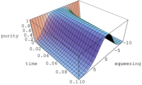
The first criterion we consider is predictability sieve. It is well known that for an underdamped harmonic oscillator at zero temperature, preferred states - as selected by the predictability sieve - are coherent states zurek93 ; coherent : these are the initial pure states that minimize the rate of purity loss. In fact, when $T=0$ they are perfect pointer states in the sense that an initial coherent state ($\alpha_{0}=\beta_{0}=1$) remains a pure coherent state with $\alpha(t)=\beta(t)=1$, see Eqs.(8), and the purity loss is identically zero goetsch1 ; goetsch2 ; giovannetti . In Fig. (1) we plot purity $P(t)=\sqrt{\alpha(t)\beta(t)}$ for zero temperature under unconditional evolution starting from initial pure states parametrized by one parameter $\kappa$ as $\alpha(0)=\kappa$, $\beta(0)=1/\kappa$. As already mentioned, the predictability sieve criterion is optimized for initial coherent states ($\kappa=1$). Now we will show that these states are also the most classical states according to three different criteria: purification time, efficiency threshold, and purity loss time. We will also show that a single measurement strategy, heterodyne detection, maximizes the robustness of all those criteria. This is expected, since heterodyne detection measures the $x$ and $p$ quadratures of the state on an equal footing, and a coherent state has equal variances of position and momentum.

Figure 1: Purity as a function of time under unconditional evolution at $T=0$ starting from an initial pure Gaussian state parametrized by a squeezing parameter $\xi=\log\kappa$. Purity is not lost for $\xi=0$, i.e., the coherent state with $(\alpha,\beta)=(1,1)$. Coherent states are perfect pointer states at $T=0$, and optimize the predictability sieve criterion. By contrast, purity is initially lost on a decoherence time scale for other states with $\xi\neq 0$. Time is measured in units of the spontaneous emission time.

The second criterion we consider is purification time. We start from a thermal state with $\alpha_{0}=\beta_{0}\ll 1$, and study how fast the state is purified by the measurement. Purity $P(t)=\sqrt{\alpha(t)\beta(t)}$ can be shown to evolve deterministically, so there is no need to do conditional stochastic simulations to study purification time. The initial rate of purity gain can be easily evaluated

$$\left.\frac{dP}{dt}\right|_{t=0}=\sqrt{\eta_{x}\eta_{y}}.$$ (10)

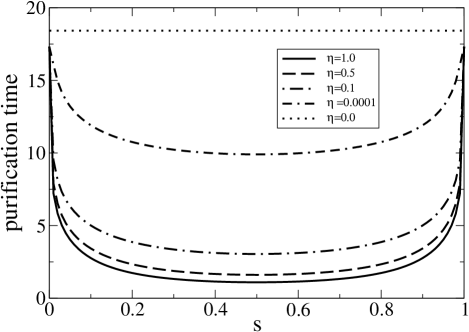
It is maximized for heterodyne detection $\eta_{x}=\eta_{y}=\eta/2$. To go beyond this simple calculation of the initial purification rate, we calculate purification time, defined as the time needed by the conditional evolution to increase purity to $P=0.5$, which is half way between the initial thermal value $P=0$, and the final pure state $P=1$ wiseman . In Fig.(1) we plot purification time for different values of the global efficiency $\eta$ as a function of the measurement scheme, parametrized by $s\in[0,1]$: $\eta_{x}=\eta\cos^{2}\left(s\frac{\pi}{2}\right)$ and $\eta_{y}=\eta\sin^{2}\left(s\frac{\pi}{2}\right)$. As expected, purification time is minimal for heterodyne detection ($s=0.5$), which corresponds to a coherent state (i.e., a pointer state).

Figure 2: Purification time as a function of the measurement scheme parametrized by $s\in[0,1]$: $\eta_{x}=\eta\sin^{2}\left(s\frac{\pi}{2}\right)$ and $\eta_{y}=\eta\cos^{2}\left(s\frac{\pi}{2}\right)$. The initial state is a fat Gaussian state $\alpha_{0}=\beta_{0}=10^{-8}$. The temperature of the bath is zero. We note that while there is a clear optimum in Fig. (1), the very best state $s=0.5$ is not all that much better than $s\sim 0.2$ or $0.8$. Thus, there is a large “quantum halo” halo of states that maintain purity well (and in this sense are reasonably classical).

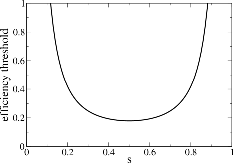
The third criterion is efficiency threshold: the minimal efficiency $\eta_{\rm thr}$ needed to reach a threshold value of purity $0<P_{\rm thr}<1$ starting from a mixed high temperature thermal state. This criterion cannot be directly used here to discriminate between different measurements because in a long time the state always relaxes to the pure vacuum state no matter what the efficiencies $\eta_{x}$ and $\eta_{y}$ are, even in the unconditional evolution . When applied literally, the criterion always gives the trivial result $\eta_{\rm thr}=0$. This is why we study a modified criterion: we measure the minimal $\eta_{\rm thr}$ needed to reach a $P_{\rm thr}$ after a time $t_{\rm thr}$. In Fig. 3 we show $\eta_{\rm thr}$ needed to reach $P_{\rm thr}=0.5$ after $t_{\rm thr}=2.5$ for different measurement schemes parametrized by $s\in[0,1]$: $\eta_{x}=\eta\cos^{2}\left(s\frac{\pi}{2}\right)$ and $\eta_{y}=\eta\sin^{2}\left(s\frac{\pi}{2}\right)$. As expected, the $\eta_{\rm thr}$ is minimal for heterodyne detection ($s=0.5$).

Figure 3: The minimal efficiency threshold $\eta_{\rm thr}$ needed to reach the threshold purity $P_{\rm thr}=0.5$ after the time $t_{\rm thr}=2.5$ as a function of the measurement scheme parametrized by $s\in[0,1]$: $\eta_{x}=\eta_{\rm thr}\sin^{2}\left(s\frac{\pi}{2}\right)$ and $\eta_{y}=\eta_{\rm thr}\cos^{2}\left(s\frac{\pi}{2}\right)$. The initial state and temperature are the same as in Fig. 1. Again, $s=0.5$ is surrounded by a sizable “halo” of (nearly) pointer states halo .

The fourth criterion is the purity loss time (proposed in wiseman , and called “mixing time” in that reference). The conditional trajectory has to evolve long enough for the state to become pure. Then one stops measuring the environment to see how fast the purity of the state decreases as a function of time, for different initial measurement schemes. All this has to be done before the state relaxes to vacuum. As already mentioned, for a high temperature initial state with $\alpha_{0}=\beta_{0}<<1$ the unconditional evolution relaxes the state to vacuum after time $\ln(1/\alpha_{0})\gg 1$. In the limit of $\alpha_{0}\to 0$ this relaxation time tends to infinity. In the same limit the conditional evolution becomes

$$\alpha(t) = \frac{e^{t}-1}{e^{t}-1+\frac{1}{\eta_{x}}},$$ (11)

$$\beta(t) = \frac{e^{t}-1}{e^{t}-1+\frac{1}{\eta_{y}}},$$ (12)

and the purity $P(t)=\sqrt{\alpha(t)\beta(t)}$ approaches $1$ after a purification time ${\rm max}\left[\ln(1/\eta_{x}),\ln(1/\eta_{y})\right]$. When both $1\geq\eta_{x},\eta_{y}\gg\alpha_{0}$, then the purification time is much shorter than the relaxation time (compare also Fig.2), and the conditional state collapses to a coherent state much faster than the relaxation time in the unconditional evolution. To measure the purity loss time once the pure coherent state is achieved, the evolution is switched to the unconditional evolution with $\eta_{x}=\eta_{y}=0$, and the purity decay is observed. However, since all measurement strategies collapse the state to a coherent state, the subsequent unconditional evolution does not destroy the purity of this state: the amplitude of the pure coherent state smoothly relaxes to the vacuum. This infinite purity loss time is the same for all measurement schemes. Coherent states, in the case of $T=0$, are perfect pointer states: once the conditional state is collapsed to a coherent state it cannot lose any purity.

II.2 Finite temperature bath

The SME for the harmonic oscillator coupled to a finite temperature bath at temperature $T$ is

$$d\rho = (n+1)D[a]\rho dt+nD[a^{\dagger}]\rho dt+$$

$$\frac{\sqrt{\eta_{x}}}{\sqrt{1+2n}}dW_{x}\left\{{\cal H}_{\phi}[(n+1)a]\rho-{\cal H}_{\phi}[na^{\dagger}]\rho\right\}+$$

$$\frac{\sqrt{\eta_{y}}}{\sqrt{1+2n}}dW_{y}\left\{{\cal H}_{\phi+\frac{\pi}{2}}[(n+1)a]\rho-{\cal H}_{\phi-\frac{\pi}{2}}[na^{\dagger}]\rho\right\},$$

where $n=(e^{\hbar\omega_{0}/k_{\rm B}T}-1)^{-1}$ is the Bose distribution. This equation is valid in the interaction picture and after the rotating wave approximation is performed. We can write the analogous equation for the Wigner distribution. We take $\phi=0$, without loss of generality, and get

$$d{\cal W}(x,p) = dt\hat{D}{\cal W}+\sqrt{\eta_{x}}dW_{x}[\hat{\cal H}_{x}{\cal W}-{\cal W}{\rm Tr}(\hat{\cal H}_{x}{\cal W})]+$$ (13)

$$\sqrt{\eta_{y}}dW_{y}[\hat{\cal H}_{y}{\cal W}-{\cal W}{\rm Tr}(\hat{\cal H}_{y}{\cal W})],$$

where now

$$\hat{\cal D}{\cal W}=\left(1+\frac{x\partial_{x}+p\partial_{p}}{2}+\frac{1+2n}{4}(\partial_{x}^{2}+\partial_{p}^{2})\right){\cal W}(x,p)dt,$$

and

$$\hat{\cal H}_{x}{\cal W} = \sqrt{2}\left(x+\frac{1}{2}(1+2n)\partial_{x}\right){\cal W}(x,p),$$

$$\hat{\cal H}_{y}{\cal W} = \sqrt{2}\left(p+\frac{1}{2}(1+2n)\partial_{p}\right){\cal W}(x,p).$$

Assuming a Gaussian Ansatz for the Wigner function we get the deterministic equations for $\alpha(t)$ and $\beta(t)$. They are the same equations as for zero temperature, with the replacement $\alpha(t)\rightarrow(1+2n)\alpha(t)$. Hence, the solution can be straightforwardly obtained from Eq.(8).

Figure 4: Purity as a function of time under unconditional evolution at finite temperature starting from an initial pure Gaussian state parametrized by the squeezing parameter $\xi=\log\kappa$. The temperature of the bath is $k_{\rm B}T/\hbar\omega_{0}=10^{6}$, where $\omega_{0}$ is the frequency of the system oscillator. Again, coherent states ($\xi=0$) are selected by predictability sieve, as they lose purity most slowly. For large times, all initial states lead to the same stationary state with purity $P(\infty)=1/(1+2n)$, where $n\approx 10^{6}$ for this temperature. Time is measured in units of the spontaneous emission time.

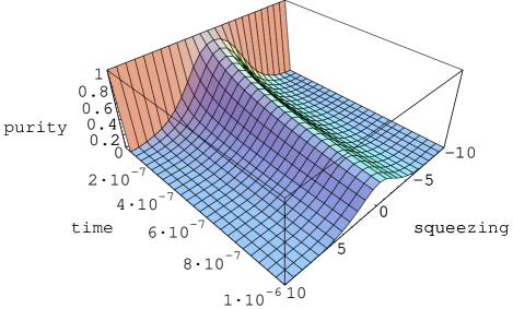
When $T>0$, the stationary state of the evolution is $\alpha_{\rm ss}=\beta_{\rm ss}=1/(1+2n)$, i.e., a Gaussian with variances in position and momentum larger than 1. The unconditional evolution relaxes to this stationary state on a time scale $t\simeq{\rm max}[\ln(1/(1+2n)\alpha_{0}),\ln(1/(1+2n)\beta_{0})]$. An initial pure coherent state $\alpha_{0}=\beta_{0}=1$ does not remain pure; it loses purity and reaches the stationary state with final purity $P(t\rightarrow\infty)=1/(1+2n)<1$. Predictability sieve still selects coherent states as pointer states, even at finite temperature (see Fig. 4). Also, heterodyne detection measurement maximizes the robustness of all the criteria (purification time, efficiency threshold, and purity loss time). For an initial high temperature state such that $(1+2n)\alpha_{0}=(1+2n)\beta_{0}\ll 1$, the unconditional evolution relaxes towards the stationary state on a very large time scale with $P(\infty)=1/(1+2n)$, while the conditional evolution reaches the same asymptotic value of purity on a much shorter time scale, of the order of ${\rm max}[\ln(1/\eta_{x}),\ln(1/\eta_{y})]$. At finite temperature, the purity loss time is not infinity as for $T=0$: all measurement schemes lead to the same, non pure state, then the measurement is switched off, and then purity is reduced again to the same final value, irrespective of the measurement scheme. This criterion cannot distinguish measurement schemes.

In summary, all classicality robustness criteria select the same states (coherent states) for the model of an underdamped harmonic oscillator, for all temperatures of the bath.

III A free particle undergoing quantum Brownian motion at high temperature

The high temperature conditional homodyne and heterodyne master equation for a free particle undergoing quantum Brownian motion is diosi ; wiseman

$$d\rho = -\frac{i}{2}\left[p^{2}+\frac{qp+pq}{2},\rho\right]dt+{\cal D}[c]\rho dt+$$ (14)

$$\left[\sqrt{\eta}\;dW\left(c\rho-\rho{\rm Tr}(\rho c)\right)+{\rm h.c.}\right]~{}.$$

Here $\eta$ is the total efficiency of the measurement, and the annihilation operator $c$ is

$$c=\frac{1}{\sqrt{2}}\left(\sqrt{4T}q+\frac{ip}{\sqrt{4T}}\right)~{}.$$ (15)

We use rescaled units such that the damping rate, the particle mass, Boltzmann constant, and $\hbar$ are all unity. The complex, Gaussian Wigner increment has correlators $\overline{dWdW^{*}}=dt$ and $\overline{dW^{2}}=dt\;re^{i\varphi}$ with $-1\leq r\leq 1$. It can be written in terms of two real, uncorrelated, Gaussian noises $dW_{x}$ and $dW_{y}$ as

$$dW=e^{+i\varphi/2}\sqrt{\frac{1+r}{2}}\;dW_{x}+e^{-i\varphi/2}\sqrt{\frac{1-r}{2}}\;dW_{y},$$ (16)

where $\overline{dW_{x}^{2}}=\overline{dW_{y}^{2}}=dt$, and $\overline{dW_{x}dW_{y}}=0$. In this way, the stochastic part of the master equation Eq.(14) can be expressed as

$$d\rho^{\rm stoch}=\sqrt{\eta_{x}}dW_{x}\;{\cal H}_{\phi}[c]\rho+\sqrt{\eta_{y}}dW_{y}\;{\cal H}_{\phi+\frac{\pi}{2}}[c]\rho.$$ (17)

Here we have defined $\phi=-\varphi/2$, $\eta_{x}=\eta(1+r)/2$, and $\eta_{y}=\eta(1-r)/2$. Heterodyne detection corresponds to $r=0$, while $r=1$ corresponds to homodyne measurement of the linear combination $ce^{i\phi}+c^{\dagger}e^{-i\phi}$ of $q$ and $p$. Hence, $\phi=0$ corresponds to a measurement of $q$, and $\phi=\pi/2$ to a measurement of $p$. The unconditional version of the master equation (14) was derived in Ref.diosi as Markovian approximation to the exact quantum Brownian motion master equation at high temperature. The equation is valid only when $T\gg 1$.

As discussed in the Introduction, the free particle undergoing quantum Brownian motion does not have well defined pointer states for any temperature of the environment. For example, at high $T$ the Lindblad term in the master equation (14) formally dominates over the free Hamiltonian part, and predictability sieve would select eigenstates of the annihilation operator $c$, that correspond to Gaussian states squeezed in position. However, this answer is not robust under variations of the time $t$ during which the criterion is applied: states squeezed in position have a large dispersion in momentum, and the free dynamical evolution will drive the state away from the squeezed eigenstates of $c$. We will show below that, because of these facts, different classicality criteria are maximized for different unravellings. However, even under these circumstances the selected states are very similar Gaussians.

Just as in the model of the underdamped harmonic oscillator, the conditional dynamics Eq.(14) preserves Gaussianity. We assume a Gaussian ansatz for the Wigner function

$${\cal W}(x,p) = \exp\left\{-\alpha(t)[x-x_{0}(t)]^{2}-\beta(t)[p-p_{0}(t)]^{2}-\right.$$ (18)

$$\left.2\gamma(t)[x-x_{0}(t)][p-p_{0}(t)]+\delta(t)\right\}.$$

The coefficients $\alpha(t)$, $\beta(t)$, and $\gamma(t)$ evolve deterministically according to the following equations

$$\frac{d\alpha}{dt} = -\frac{\alpha^{2}}{4T}-4T\gamma^{2}+4T\eta_{x}A_{1}^{2}+4T\eta_{y}A_{2}^{2},$$ (19)

$$\frac{d\beta}{dt} = -4T\beta^{2}-\frac{\gamma^{2}}{4T}+2\beta-2\gamma+\frac{\eta_{x}}{4T}B_{1}^{2}+\frac{\eta_{y}}{4T}B_{2}^{2},$$

$$\frac{d\gamma}{dt} = -\frac{\alpha\gamma}{4T}-4T\beta\gamma+\gamma-\alpha+\eta_{x}A_{1}B_{1}-\eta_{y}A_{2}B_{2},$$

where

$$A_{1} = \gamma\sin\phi-\left(1-\frac{\alpha}{4T}\right)\cos\phi,$$

$$A_{2} = \gamma\cos\phi+\left(1-\frac{\alpha}{4T}\right)\sin\phi,$$

$$B_{1} = \gamma\cos\phi-\left(1-4T\beta\right)\sin\phi,$$

$$B_{2} = \gamma\sin\phi+\left(1-4T\beta\right)\cos\phi.$$

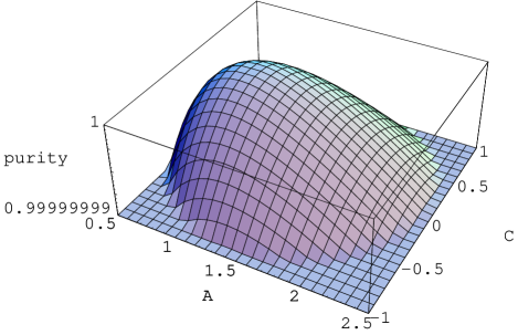
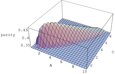
To apply the predictability sieve criterion we solve the unconditional version of these equations ($\eta_{x}=\eta_{y}=0$) starting from different initial pure Gaussian states. The initial pure state is parametrized by two parameters $(A,C)$ as $\alpha(0)=4T~{}A,\gamma(0)=C$ and $\beta(0)=[1+\gamma^{2}(0)]/\alpha(0)$. In this parametrization the squeezed eigenstate of $c$ is $(A=1,C=0)$. In figure 5 we show purity $P(t)=\sqrt{\alpha(t)\beta(t)-\gamma^{2}(t)}$ after unconditional evolution for a very short time $t=0.1/4T=2.5~{}10^{-8}$ at temperature $T=10^{6}$ as a function of initial pure state $(A,C)$. Purity is maximal when $(A,C)$ are approximately equal to $(1,0)$, i.e., purity is maximized for the eigenstate of the squeezed operator $c$ with $(\alpha,\beta,\gamma)=(4T,1/4T,0)$. As expected, at early times the evolution is dominated by the Lindblad term and it is most predictable for the eigenstates of $c$. In the high-$T$ limit these eigenstates tend to be position eigenstates. However, the range of values of purity in figure 5 is only $(0.99999999,1)$, so that after this short time the evolution is still very predictable no matter what the initial state is - the most robust states are not well distinguished from the rest.

Rather than the early times $t\simeq 1/4T$ we found the times $t\simeq 1/\sqrt{4T}$ more relevant from the point of view of predictability sieve, since then the unconditional evolution starting from the most robust initial states loses approximately one half of its initial purity, while at the same time the evolution starting from bad states is essentially not predictable at all. At $t\simeq 1/\sqrt{4T}$ the most robust states are well distinguished from “the Hilbert space chaff” by the predictability sieve. In figure 6 we show purity $P(t)$ after unconditional evolution at temperature $T=10^{6}$ at a time $t=2/\sqrt{4T}=10^{-3}$. Purity is maximal when $(A,C)=(1.75,1.75)$ or $(\alpha,\beta,\gamma)=(1.75\sqrt{4T},\frac{2.32}{\sqrt{4T}},1.75)$. In the high $T$ limit these states are very different from the eigenstates of $c$ although they also tend to approximate position eigenstates for large values of the temperature. In a strict sense predictability sieve does not select any well defined and $t$-independent pointer states. Nevertheless, non-local superpositions are still quickly destroyed, and lose purity much faster than the stable and more or less localized Gaussians we have described. Therefore, for many practical purposes the states which are selected at measurement times $t\simeq 1/\sqrt{4T}$ may play the role of the robust classical states. Parameters of these states scale with $T$ as $\alpha\simeq\sqrt{4T}$, $\beta\simeq\frac{1}{\sqrt{4T}}$, and $\gamma\simeq 1$. In the following we will see that this class of states is also preferred by the other classicality criteria.

Figure 5: Purity under unconditional evolution at $T=10^{6}$ after a short time $t=0.1/4T=2.5~{}10^{-8}$ starting from an initial pure Gaussian state parametrized by two numbers $(A,C)$. The parameter $A$ is related to the squeezing of the probability distribution of the initial state, and $C$ is related to its tilt in phase space. Purity is maximized for an initial state that is approximately parametrized by $(A,C)=(1,0)$, that is, the eigenstate of the squeezed annihilation operator $c$ with $(\alpha,\beta,\gamma)=(4T,\frac{1}{4T},0)$, which is the most predictable state after this short time of unconditional evolution. However, the vertical range of the plot is only $(0.99999999,1)$ - at this early time the unconditional evolution is still very predictable no matter what its initial pure state is. The most predictable eigenstates of $c$ are not well distinguished from the rest. Rescaled units are used.

Figure 6: Purity after unconditional evolution at $T=10^{6}$ for a time $t=2/\sqrt{4T}=10^{-3}$ when the unconditional evolution starting from the most robust initial state loses approximately one half of its initial purity. Purity is maximal when $(A,C)=(1.75,1.75)$, or $(\alpha,\beta,\gamma)=(1.75\sqrt{4T},\frac{2.32}{\sqrt{4T}},1.75)$. At this time the most predictable initial states are well distinguished from (are much more pure than) other states, which already have negligible purity. Rescaled units are used.

Now we turn to the second classicality criterion, purification time. In order to quantify it we prepare the system in its unconditional stationary thermal state, $\alpha_{0}=\gamma_{0}=0,\beta_{0}=1/2T$. Then we compute how fast the conditional state is gaining purity $P(t)$ depending on the measurement scheme on the environment, defined by $r$ and $\phi$. Here we assume full efficiency ($\eta=1$). The initial rate of gain of purity can be easily calculated analytically at $t=0$:

$$2P(0)\dot{P}(0)=\left.\left(\beta\frac{d\alpha}{dt}+\alpha\frac{d\beta}{dt}-2\gamma\frac{d\gamma}{dt}\right)\right|_{t=0}=1+r\cos 2\phi$$

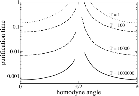
and it is found not to depend on $T$. This initial purification rate is fastest when $r=1$ and $\phi=0,\pi$, or when $r=-1$ and $\phi=\pi/2,3\pi/2$. All these four solutions correspond, in fact, to the same $x-$homodyne. The slowest initial purification is obtained for $y-$homodyne with $r=1,\phi=\pi/2$. To go beyond the initial purification we measure the purification time, defined as the time needed by the fully efficient ($\eta=1$) conditional evolution to increase purity to $P=0.5$, which is half way between the initial thermal state value ($P\approx 0$) and the final pure state value ($P=1$) wiseman . Purification times for different homodyne angles $\phi$ at different temperatures are shown in figure 7. As expected, purification time is the shortest for $x-$homodyne, i.e., when $r=1$ and $\phi=0,\pi$. In contrast, $y-$homodyne does not purify the state at all.

Figure 7: Purification time as a function of the homodyne angle $\phi$ ($r=1$) for an initial thermal state with temperature $T$. Purification time is the shortest for $x-$homodyne, i.e., when $\phi=0,\pi$. By contrast, $y-$homodyne ($\phi=\pi/2$) does not purify the state at all. Rescaled units are used.

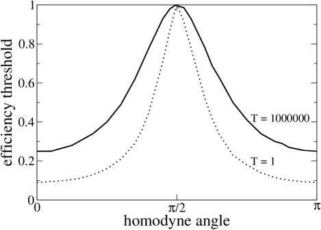
Now we consider the efficiency threshold, defined as the minimal efficiency $\eta_{\rm thr}$ required for the conditional evolution to asymptotically reach a threshold purity $P_{\rm thr}$. Here we assume $P_{\rm thr}=0.5$ and an initial thermal state. Efficiency thresholds for different homodyne angles $\phi$ are collected in Figure 8. The threshold is the lowest for $x-$homodyne ($\phi=0,\pi$), and the highest for $y-$homodyne when full efficiency is required to find out the state after infinitely long time.

Figure 8: Efficiency threshold as a function of the homodyne angle $\phi$ for an initial thermal state with temperature $T$. The threshold is the lowest for $x-$homodyne ($\phi=0,\pi$) and the highest for $y-$homodyne ($\phi=\pi/2$). Rescaled units are used.

Finally, in order to measure the purity loss time (called “mixing time” in wiseman ), we evolve the conditional state of the system for a sufficiently long time so that it reaches a conditional stationary state, that depends on the measurement scheme. The stationary conditional state can be obtained by setting the left hand sides of Eqs. (19) to zero and solving the equations for $\alpha_{\rm ss},\beta_{\rm ss},\gamma_{\rm ss}$. In the high $T$ limit, the stationary solutions can be found in the form $\alpha_{\rm ss}=A_{\rm ss}\sqrt{4T},\beta_{\rm ss}=B_{\rm ss}/\sqrt{4T},\gamma_{\rm ss}=C_{\rm ss}$. After keeping in each equation only the leading order terms in the high $T$ limit we obtain simplified equations for $A_{\rm ss},B_{\rm ss},C_{\rm ss}$, and their solution gives,

$$A_{\rm ss} = -\frac{B_{\rm ss}C_{\rm ss}}{2}(1+r\cos 2\phi)-\frac{B_{\rm ss}}{2}r\sin 2\phi,$$

$$B_{\rm ss} = \left(-\frac{4C_{\rm ss}}{1+r\cos 2\phi}\right)^{1/2},$$

$$C_{\rm ss} = -\frac{r\sin 2\phi+\sqrt{1+2r\cos 2\phi+r^{2}}}{1+r\cos 2\phi}.$$ (20)

Once the stationary state is achieved the evolution is switched to unconditional evolution with $\eta=0$ and we calculate the purity loss rate. This depends on the measurement scheme through the stationary conditional state, which is the initial state for the unconditional evolution. The initial purity loss rate can be easily calculated as

$$\left.-\frac{dP}{dt}\right|_{t=0}=\sqrt{T}\;B_{\rm ss},$$ (21)

to leading order in high $T$. This initial purity loss rate is minimized for $x-$homodyne with $r=1$ and homodyne angle $\phi=5\pi/6$.

Figure 9: Purity loss time needed by unconditional evolution to reduce purity from the initial value $P=1$ to $P=0.5$, which is half way to the stationary value $P=0$ in the thermal state. The homodyne angle that maximizes the purity loss time is $\phi=1.35~{}\frac{\pi}{2}$. On the other hand, the purity loss time is zero for $y-$homodyne with $\phi=\pi/2$. Rescaled units are used.

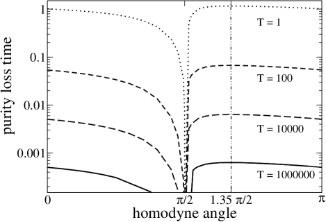
So far we have analyzed only the initial purity loss time. Now we consider the purity loss time, defined as the time needed by the unconditional evolution to reduce purity to $P=0.5$, which is half way between the initial pure state and the stationary thermal state with $P\approx 0$. In figure 9 we show the purity loss time as a function of homodyne angle $\phi$ after homodyne measurement with $r=1$. The homodyne angle that maximizes the purity loss time is $\phi=1.35\pi/2$.

Figure 10: Wigner functions of the stationary conditional states selected at high temperatures $T=10^{6}$ by different robustness criteria: (a) purification time and efficiency threshold (homodyne angle $\phi=0$), and (b) purity loss time (homodyne angle $\phi=1.35\pi/2$). The two selected states are very similar (scalar product equal to $0.97$), and Gaussians squeezed to “approximate” position eigenstates. Rescaled units are used.

Figure 11: Wigner functions of the stationary conditional states selected at low temperatures $T=1$ by different robustness criteria: (c) purification time and efficiency threshold (homodyne angle $\phi=0$), and (d) purity loss time (homodyne angle $\phi=1.35\pi/2$). The two selected states are very similar (scalar product equal to $0.99$), and approximately equal to coherent states with $\alpha=\beta=1$, $\gamma=0$ (scalar product with a coherent state is equal to $0.99$ and $0.98$ respectively). Rescaled units are used.

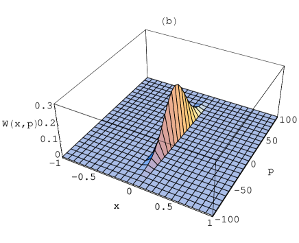
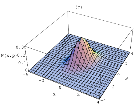
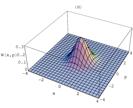
We applied the three different criteria and we found that in two cases - purification time and efficiency threshold - the most robust measurement strategy is $x-$homodyne ($\phi=0$) over the whole range of temperatures, but in one case - purity loss time - the most robust measurement is homodyne with $\phi=1.35\pi/2$. In each case the most robust measurement defines the most classical state as the conditional stationary state obtained with the optimal measurement scheme.These results may leave one under the impression that various criteria lead to different candidates for classical states. Indeed, this was the conclusion of wiseman , where similar results concerning optimal measurement strategies were obtained for the model of this Section. The key point is, however, that although different classicality criteria are maximized by different measurement strategies, in all cases the states that are singled out are almost identical.

In the two following tables we list parameters of the conditional stationary states for $\phi=0$ and $\phi=1.35\pi/2$ for several values of the temperature. The states can be described by three independent quantities: the dispersions in position $\Delta x$ and in momentum $\Delta p$, and the covariance $C_{xp}\equiv\langle xp+px\rangle/2-\langle x\rangle\;\langle p\rangle$. We find that for all listed temperatures the stationary conditional states for $\phi=0$ and $\phi=1.35\pi/2$ are very similar (see figures 6 and 7). One can easily imagine they are well within each others “quantum halo” halo . These states evolve from almost coherent at $T=1$ to almost position eigenstates at high $T$. Thus, in contrast to wiseman , we conclude that all of the above criteria lead to essentially the same “most classical” states.

Table 1: Stationary conditional state for homodyne angle $\phi=0$ at different temperatures $T$. Rescaled units are used.

$T$	$\alpha_{\rm ss}$	$\beta_{\rm ss}$	$\gamma_{\rm ss}$	$\Delta x$	$\Delta p$	$C_{xp}$
$10^{6}$	$2826$	$0.0007$	$-0.999$	$0.018$	$37.968$	$0.509$
$10^{4}$	$280$	$0.0070$	$-0.992$	$0.059$	$11.977$	$0.508$
$10^{2}$	$26.4$	$0.0707$	$-0.931$	$0.188$	$3.633$	$0.466$
$1$	$1.53$	$0.8002$	$-0.480$	$0.632$	$0.877$	$0.241$

Table 2: Stationary conditional state for homodyne angle $\phi=1.35\pi/2$ at different temperatures $T$. Rescaled units are used.

$T$	$\alpha_{\rm ss}$	$\beta_{\rm ss}$	$\gamma_{\rm ss}$	$\Delta x$	$\Delta p$	$C_{xp}$
$10^{6}$	$1500$	$0.0007$	$-0.281$	$0.018$	$27.792$	$0.144$
$10^{4}$	$149$	$0.0072$	$-0.280$	$0.060$	$8.656$	$0.141$
$10^{2}$	$14$	$0.0741$	$-0.270$	$0.192$	$2.694$	$0.140$
$1$	$1.05$	$0.9561$	$-0.112$	$0.694$	$0.728$	$0.056$

IV Conclusions

In the example of the under-damped harmonic oscillator, where pointer states defined by the predictability sieve criterion are unambiguous, we have shown that different classicality criteria single out the same states, i.e., coherent states that coincide with the pointer states selected by the predictability sieve zurek93 ; coherent . We considered three of these “alternative classicality criteria”: purification time, which looks for states of the system that are the easiest to find out from the imprint they leave on the environment; efficiency threshold, which finds states of the system that can be deduced from measurements on a smallest fraction of the environment; and purity loss time, that looks for states of the system for which it takes the longest to lose a set fraction of their initial purity. Our findings indicate that quantum unravelings are in effect classical for pointer states.

When pointer states are not well defined, as in the model of a free particle undergoing quantum Brownian motion, or when pointer states do not exist at all, different criteria may select different states. However, it appears that these candidate classical states are very similar, defining approximate pointer states, as in the model of the free particle undergoing quantum Brownian motion. This is an interesting example because different classicality criteria select measurement schemes that appear quite different, but these different schemes turn out to prepare very similar Gaussian states.

Following our work ourprl , the classical robustness of different quantum unravellings was studied in wiseman , where some of the classicality measures used in this paper – such as efficiency threshold and purity loss time (called “mixing time” in wiseman ) – were considered. It was claimed there that for a fixed environmental interaction the level of robustness depends on the measurement strategy, and that no single strategy is maximally robust in all ways. This conclusion was drawn from two models: resonance fluorescence of a two-level atom (a model for which pointer states do not exist), and a free particle in quantum Brownian motion (one of the models used in this paper, for which one might perhaps argue there are approximate, time-dependent, and imperfect pointer states). As we discussed above, the conclusion of Ref.wiseman does not apply to the case when einselection works well, i.e., when pointer states are well defined (e.g., the under-damped harmonic oscillator). Moreover, the conclusion of wiseman is misleading even for the example of the free particle undergoing quantum Brownian motion they have investigated: Pointer states are not well defined there, and different robustness criteria are optimized by different measurement strategies. Yet, the states resulting from all of the above strategies are essentially identical! Thus, even when einselection does not pick out unique pointer states, different criteria still agree on what appears to be most classical.

Our conclusions may assist in the choice of the optimal measurement strategies, especially in applications that involve quantum control. The fact that when good or even approximate pointer states exist, they tend to be prepared by all the seemingly different schemes optimized for several reasonable criteria, attest to the practical implications of their classicality.

V Acknowledgments

We are grateful to Howard M. Wiseman for fruitful discussions and correspondence. This work was supported in part by NSA.

References

- (1) W.H. Zurek, Phys. Rev. D 24, 1516 (1981).
- (2) W.H. Zurek, Phys. Rev. D 26, 1862 (1982).
- (3) W.H. Zurek, Prog. Theor. Phys. 89, 281 (1993).
- (4) W.H. Zurek, S. Habib, and J.P. Paz, Phys. Rev. Lett. 70, 1187 (1993).
- (5) M.R. Gallis, Phys. Rev. A 53, 655 (1996).
- (6) M. Tegmark and H.S. Shapiro, Phys. Rev. E 50, 2538 (1994).
- (7) J.P. Paz and W.H. Zurek, in Coherent Matter Waves, Les Houches Summer School, Session LXXII, edited by R. Kaiser, C. Westbrook, and F. David (Springer-Verlag, Berlin, 2001). pp. 533-614.
- (8) E. Joos, H.D. Zeh, C. Kiefer, D. Giulini, J. Kupsch, and I.-O. Stamatescu, Decoherence and the Appearance of a Classical World in Quantum Theory (Springer, Berlin, 2003).
- (9) W.H. Zurek, Rev. Mod. Phys. 75, 715 (2003).
- (10) H.M. Wiseman and J.A. Vaccaro, Phys. Lett. A 250, 241 (1998).
- (11) H.M. Wiseman and Z. Brady, Phys. Rev. A 62, 023805 (2000).
- (12) D.A.R. Dalvit, J. Dziarmaga, and W.H. Zurek, Phys. Rev. Lett. 86, 373 (2001).
- (13) W.H. Wiseman and J.A. Vaccaro, Phys. Rev. A 65, 043606 (2002).
- (14) J. Dziarmaga, D.A.R. Dalvit, and W.H. Zurek, Phys. Rev. A 69, 022109 (2004).
- (15) D.J. Atkins, Z. Brady, K. Jacobs, and H.M. Wiseman, Europhys. Lett. 69, 163 (2005).
- (16) W.H. Zurek, Annalen der Physik 9, 855 (2000).
- (17) H. Ollivier, D. Poulin, and W.H. Zurek, Phys. Rev. Lett. 93, 220401 (2004); also quant-ph/0408125.
- (18) R. Blume-Kohout and W.H. Zurek, quant-ph/0408147; quant-ph/0505031.
- (19) L. Diósi, Phys. Lett. A 129, 419 (1988); A. Barchielli and V.P. Belavkin, J. Phys. A 24, 1495 (1991); J. Dalibard, Y. Castin, and K. Molmer, Phys. Rev. Lett. 68, 580 (1992); C.W. Gardiner, A.S. Perkins, and P. Zoller, Phys. Rev. A 46, 4363 (1992); N. Gisin and I.C. Percival, J. Phys. A 25, 5677 (1992); H. Carmichael, An Open Systems Approach to Quantum Optics (Springer, Berlin, 1993); R. Schack, T.A. Brun, and I.C. Percival, J. Phys. A 28, 5401 (1995); H.J. Carmichael, ed., Quant. Semiclass. Opt. 8, no. 1 (1996); I.C. Percival, Quantum State Diffusion (Cambridge University Press, Cambridge, 1998).
- (20) T. Bhattacharya, S. Habib, and K. Jacobs, Phys. Rev. Lett. 85, 4852 (2000).
- (21) H.M. Wiseman and G.J. Milburn, Phys. Rev. A 47, 1652 (1993).
- (22) H.M. Wiseman and L. Diósi, Chem. Phys. 268, 91 (2001).
- (23) P. Goetsch, P. Tombesi, and F. Haake, Phys. Rev. A 51, 136 (1995).
- (24) P. Goetsch, P. Tombesi, and D. Vitali, Phys. Rev. A 60, 4519 (1996).
- (25) V. Giovannetti, P. Tombesi, and D. Vitali, Phys. Rev. A 60, 1549 (1999).
- (26) J.R. Anglin and W.H. Zurek, Phys. Rev. D 53, 7327 (1996).
- (27) L. Diósi, Europhys. Lett. 22, 1 (1993).