Homodyne measurement of average photon number

Abstract

We describe a new scheme for the measurement of mean photon flux at an arbitrary optical sideband frequency using homodyne detection. Experimental implementation of the technique requires an AOM in addition to the homodyne detector, and does not require phase locking. The technique exhibits polarisation, frequency and spatial mode selectivity, as well as much improved speed, resolution and dynamic range when compared to linear photodetectors and avalanche photo diodes (APDs), with potential application to quantum state tomography and information encoding using an optical frequency basis. Experimental data also directly confirms the Quantum Mechanical description of vacuum noise.

I Introduction

The most fundamental optical measurement is the intensity of a specific mode. Quantum optics tells us that the intensity is quantized WallsMilburn , appearing as a discrete photon flux. For a sufficiently small flux the individual photons can be resolved and counted using a number of standard techniques such as avalanche photodiodes (APDs), photomultipliers and bolometers ZambraPRL . The optimum approach for a given application is dependent upon the wavelength and expected photon flux. An important point is that at optical frequencies the thermal background is at zero temperature to an excellent approximation. Thus ”dark counts”, i.e. photon events in the absence of illumination, are technical in nature.

It is also possible to probe an optical mode by first mixing it with a strong reference field, a local oscillator, before detecting its intensity. This is called homodyne detection. In this case detection is generally by linear positive-intrinsic-negative (PIN) photodiode detectors which cannot resolve individual photons. Instead, the continuous spectrum of the signal’s quadrature amplitudes are measured. Quantum optics tells us that the quadrature amplitudes exhibit zero temperature fluctuations, thus a fundamental noise floor is observed for homodyne detection in the absence of signal illumination.

Although all this is well known and the performance of photon counters and homodyne detectors has been tested individually for many systems BachorRalph , to our knowledge a direct comparison of the photon counting and homodyne signal of the same field has not been made. This is perhaps why some authors claim that the homodyne statistics obtained in some continuous variable quantum information experiments are inconclusive CavesPRL04 . In this paper we make such a direct comparison.

The paper is laid out in the following way. In section II we detail the theoretical relationship between continuous variable homodyne detection and the direct measurement of average photon flux densities. The experimental approach used for homodyne detection is described in Section III and the results are compared with the measurements using a single photon detector (SPDM) in Section IV. Finally, a discussion of the significance of the results is given in Section V.

As well as the fundamental interest of our results the demonstrated technique is shown to be easy to add to existing experiments, providing fast measurements over a wide dynamic range. This potentially provides for significant reductions in the time taken to construct the density matricies for qudit systems ThewPRA02 and other applications in quantum tomography.

II Theory

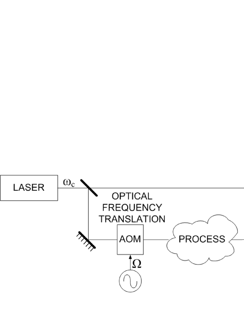
Figure 1: Generic measurement concept, as applied to determine $\bar{n}$ at the output of an unknown process. The direction of optical frequency translation as performed by the AOM is unimportant, as discussed in the text.

The annihilation and creation operators of an arbitrary field may be expressed in the Heisenberg picture as a sum of the amplitude $\hat{X_{A}^{+}}$ and phase $\hat{X_{A}^{-}}$ quadrature operators, where the annihilation $\hat{A}$ and creation $\hat{A}^{\dagger}$ operators are given by WallsMilburn

$$\begin{array}[]{c}\hat{A}=\frac{\hat{X_{A}^{+}}-i\hat{X_{A}^{-}}}{2}\\ \hat{A}^{\dagger}=\frac{\hat{X_{A}^{+}}+i\hat{X_{A}^{-}}}{2}\end{array}$$

The quadrature operators represent continuous variable observables that are able to be measured via homodyne detection techniques.

If the field operator is expressed as a linear sum of steady state coherent amplitude $\bar{A}$ and quantum mechanical fluctuation terms $\hat{\delta A(t)}$ such that $\hat{A}(t)=\bar{A}+\delta\hat{A}(t)$ and $\hat{A}(t)^{\dagger}=\bar{A}+\delta\hat{A}(t)^{\dagger}$, and use is made of the Fourier transform relationship $\hat{A}(t)\to\delta\tilde{A}(\omega)$ and $\hat{A}(t)^{\dagger}\to\delta\tilde{A}(-\omega)^{\dagger}$, then the power spectrum of the fluctuations of an arbitrary input field can be written EHHetal05 :

$$V^{\pm}(\omega) = \langle\delta\tilde{A}(\omega)^{\dagger}\delta\tilde{A}(\omega)+\delta\tilde{A}(-\omega)^{\dagger}\delta\tilde{A}(-\omega)$$ (1)

$$\pm\delta\tilde{A}(-\omega)\delta\tilde{A}(\omega)\pm\delta\tilde{A}(-\omega)^{\dagger}\delta\tilde{A}(\omega)^{\dagger}\rangle$$

$$+1$$

where the spectral variance $V^{\pm}(\omega)$ is given by $\langle|\delta X^{\pm}(\omega)|^{2}\rangle$. The first term of Eqn. 1 is the average number of photons $\bar{n}_{+}$ in the input mode at frequency $+\omega$, the second represents $\bar{n}_{-}$ at $-\omega$ and the third and fourth terms represent correlations between the $+\omega$ and $-\omega$ sidebands. The final unit term represents the vacuum fluctuations. In general, this may be expressed as TCRprl00 :

$$\bar{n}(\omega)=\frac{V^{+}(\omega)+V^{-}(\omega)-2}{4}$$ (2)

where $\bar{n}(\omega)=(\bar{n}_{+}+\bar{n}_{-})/2$ represents the average number of photons in both the positive and negative sidebands for a continuous variable measurement of the variances at frequency $\omega$. Note that this relationship also remains valid for any pair of orthogonal measurements of the optical phase space, i.e. $V^{\theta}$ and $V^{\theta+\frac{\pi}{2}}$. In this case, $V^{\theta}(\omega)=\langle|\delta\tilde{X}^{\theta}(\omega)|^{2}\rangle$ where $\delta\hat{X}^{\theta}=(\delta\hat{a}e^{i\theta}+\delta\hat{a}^{\dagger}e^{-i\theta})$, representing an arbitrary quadrature operator at angle $\theta$ with respect to a specified phase reference.

As a first example consider a coherent state $|\alpha\rangle$. Coherent states can be defined as eigenstates of the annihilation operator, i.e. $\hat{A}|\alpha\rangle=\alpha|\alpha\rangle$. To a good approximation such states can be produced by a well stabilized laser. We have $V^{+}=4Re(\alpha)^{2}+1$ and $V^{-}=4Im(\alpha)^{2}+1$. Using Eqn. 2 we find $\bar{n}=Re(\alpha)^{2}+Im(\alpha)^{2}=|\alpha|^{2}$ which is as expected.

As another example, consider the homodyne measurement of a squeezed state $|\alpha,r\rangle$. Squeezed states can be defined as eigenstates of the operator $\hat{B}=\sqrt{G}-\sqrt{G-1}$. Such a state possesses the following properties WallsMilburn :

$$\begin{array}[]{c}\Delta X^{+}=e^{-r},\quad\Delta X^{-}=e^{r}\\ \langle N\rangle=|\alpha|^{2}+\sinh^{2}r\end{array}$$

where the squeeze factor $r=-\ln(\sqrt{G}-\sqrt{G-1})$. Assuming a similarly squeezed vacuum state (i.e. $\alpha=0$) with variances $V^{+}$ and $V^{-}$ measured at frequency $\omega$, Eqn. 2 yields:

$$\bar{n}(\omega) = \frac{|e^{-r}|^{2}+|e^{r}|^{2}-2}{4}$$

$$= \left(\frac{e^{-r}-e^{r}}{2}\right)^{2}$$

$$= |0|^{2}+\sinh^{2}r$$

again in agreement with the expected result. The interesting thing in this second example is that the fluctuations in one quadrature can fall below the level associated with no illumination. This example shows that the vacuum noise floor cannot be attributed to technical noise of the detector.

The relationship of Eqn. 2 may also be exploited to measure the average photon number in a field of interest using the scheme illustrated in Fig. 1. In order to avoid low frequency technical noise, an acousto-optic modulator (AOM)KorpelAOM81 introduces a radio frequency offset $\omega$ between the mode of interest and a homodyne detector local oscillator. As shown, the mode of interest is upshifted relative to the local oscillator, and the vacuum mode introduced at frequency $-\omega$ relative to the local oscillator. From Eqn. 1, $\langle\delta\tilde{A}(-\omega)^{\dagger}\delta\tilde{A}(-\omega)\rangle=\langle\delta\tilde{A}(-\omega)\delta\tilde{A}(\omega)\rangle=\langle\delta\tilde{A}(-\omega)^{\dagger}\delta\tilde{A}(\omega)^{\dagger}\rangle=0$ and local oscillator phase dependance disappears. Consequently, $V^{+}=V^{-}$ and Eqn. 2 yields:

$$\bar{n}_{+}(\omega)=\langle\delta\tilde{A}(\omega)^{\dagger}\delta\tilde{A}(\omega)\rangle=V(\omega)-1$$ (3)

where $\bar{n}_{+}(\omega)$ is the average number of photons in the $+\omega$ sideband. A similar result is obtained if the $+\omega$ and $-\omega$ sidebands are interchanged, i.e. upshifting the local oscillator with respect to the field of interest.

III Experiment

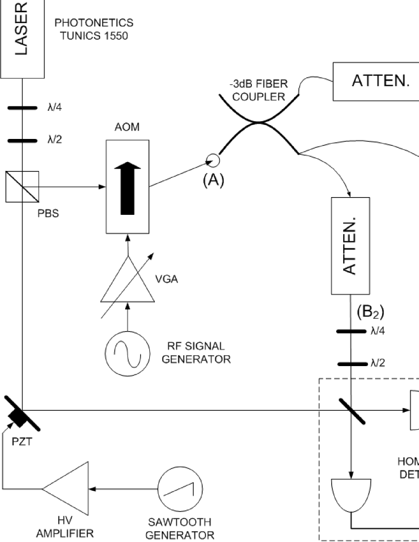
Figure 2: Schematic representation of the system employed, modematching optics omitted for clarity. Points $A$, $B_{1}$ and $B_{2}$ represent the states to be measured.

The experimental setup illustrated in Fig. 2 was an implementation of the topology shown in Fig. 1. The experiment was driven by a Photonetics Tunics-1550 tunable diode laser operated at 1540 nm, the wavelength chosen to permit stable mode-hop-free operation, as well as to take advantage of commercial telecommunications fiber products. The output beam was divided asymmetrically, the majority of the power used as a coherent local oscillator for the homodyne detector and the remainder upshifted and attenuated to become the field of interest. The field of interest was then measured by three independent detection systems; a homodyne detector, an id-Quantique (id-200) InGaAs/InP SPDM and a NIST-traceable (Newport 3227) power meter. All interconnections were made with single mode glass fiber (SMF) in the interests of reproducibility of measurement and for spatial mode filtering.

To permit valid comparisons to be made between the three measurement techniques, all measurements were referred back to Point (A) of Fig. 2, accounting for the losses unique to each optical path in the analysis of results. As physical disturbance of the SMF altered the polarisation of the propagating photons via the stress-optic effect Saleh91 , a series of data was recorded using a 50/50 fiber coupler to permit simultaneous SPDM and homodyne measurements to be made whereby the signal path waveplates had been previously adjusted for maximum homodyne efficiency. This also made long time constant drifts in the laser’s output power common to both measurement systems. However, to support the claim that both measurement schemes were truly independent, a small set of results were collected by interchanging the connections of one port of the coupler between the SPDM and the homodyne detector.

Experimentally, measurement of the mean photon number is determined by integrating the mean photon flux $\Phi$ over time period $\tau$. The field of interest at point (A) may be approximated as a weak coherent state $|\alpha\rangle_{A}$, defined WallsMilburn as

$$|\alpha\rangle=e^{\frac{-|\alpha|^{2}}{2}}\sum_{n=0}^{\infty}\frac{\alpha^{n}}{\sqrt{n!}}|n\rangle$$ (4)

where the mean photon flux is related by $\Phi=|\alpha|^{2}=P\lambda/hc$ where $P$ is the optical power, $\lambda$ is the optical wavelength, $h$ is Planck’s constant and $c$ is the speed of light.

$|\alpha\rangle_{A}$ is further attenuated in a calibrated fashion to yield $|\alpha\rangle_{B_{1,2}}$ with $\alpha_{B_{1,2}}$ varied by adjusting the RF drive power to the AOM to yield values for $\Phi_{B_{1,2}}$ in the range $\sim 10^{3}\to 10^{5}$ photons/sec. The second order Bragg-diffracted YoungAOM81 optical output was used to achieve a greater attenuation than was otherwise possible with the first order output, and to avoid radiative coupling between the RF signal generator and the homodyne detector. Hence, the AOM was operated at its frequency of peak diffraction efficiency of 80 MHz, and homodyne detection performed at a center frequency of 160 MHz.

The homodyne detector was implemented with matched InGaAs PIN photodetectors and an Agilent E4407B spectrum analyser (SA). Free space optical components were used to permit independent control of input polarisation and relative phase, the latter via a PZT mounted mirror.

As the standard deviation $\sigma_{n}$ of the Poissonian distribution described in Eqn. 4 is related to the mean photon count $\bar{n}$ by $\sigma_{n}^{2}=\bar{n}$, the variance of the SPDM measurements is reduced by maximising $\tau$. Integration times of 5 minutes with an APD gating period $\tau_{G}$ of 100 ns at 10 $\mu$s intervals were used to satisfy the practical constraints imposed by long time constant laser power drifts and afterpulsing probability APDjModO01 . The dynamic range of the SPDM measurements were restricted to only three orders of magnitude, the upper limit imposed by saturation of the APD gated time bins and the non-linearity associated with the increasing probability of $\geq 2$ photons arriving within each gate window. The lower limit arises as a consequence of the finite dark count probability and low observed SPDM quantum efficiency $\eta_{S}$ of 11%.

Homodyne measurements were performed with a nominal SA resolution bandwidth (RBW) of 30 Hz and measured RBW of 33.18 Hz. This corresponds to an effective integration time of $\tau/RBW$ = 30.1 ms, data collected for a 30 s period. The overall efficiency of the homodyne detector $\eta$ is a function of the quantum efficiency $\eta_{det}$ of the matched PIN photodetectors and the interferometric fringe visibility $VIS$, where $\eta_{H}=VIS^{2}$ and $\eta=\eta_{H}\eta_{det}$. Accounting for the transition from fiber to free space, the maximum experimental fringe visibility attained was 93%, the corrected mean photon number observed by the homodyne detector thus given by Eqn. 3, scaled by $RBW/\eta$.

IV Results

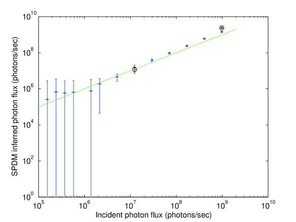
Figure 3: Average photon number at point (A) of Fig. 2, as determined by SPDM measurements.

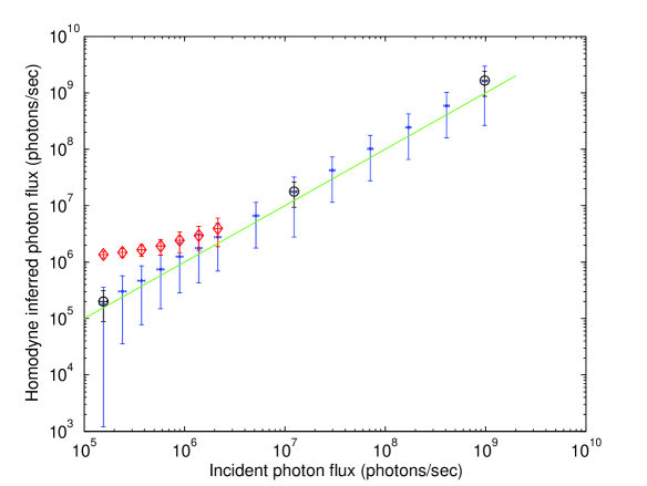
Figure 4: Average photon number at point (A) of Fig. 2, as determined by homodyne detection techniques.

Fig. 3 illustrates the SPDM inferred mean photon flux, showing a useful linear relationship over approximately 3 orders of magnitude, with the measurement uncertainty increasing rapidly at low light levels. Following the correction of technical noise as detailed in the following section, data points with a negative mean have been deleted and error bars truncated at $\Phi=0$.

Note that for both plots, the incident photon flux was determined as per Fig. 2 via macroscopic power measurements and the solid line represents the ideal 1:1 relationship between incident and measured values. The error bars for both axes are placed one standard deviation from the mean. Data points obtained via the coupler are marked with a point, the circled points (seen at incident fluxes of $1.6\times 10^{5}$, $8.0\times 10^{6}$ and $9.8\times 10^{8}$ photons/sec.) represent data obtained by interchanging connections as detailed in the proceeding section.

The homodyne detector results are shown in Fig. 4, the point/circled data values determined via Eqn. 3 exhibiting a comparatively superior dynamic range in excess of 4 orders of magnitude. If the subtraction of the vacuum noise contribution is neglected as required by stochastic electrodynamics then Eqn. 3 reduces to $\bar{n}(\omega)=V(\omega)$, the consequence of this alteration illustrated by the diamond data points. Is is observed that whilst the magnitude of the uncertainties are reduced, the results clearly disagree with both the SPDM data in Fig. 3 and the desired 1:1 relationship. Although the two sets of results converge at higher flux levels where the magnitude of vacuum noise ceases to be significant compared with the measured variance, low flux levels are only calculated correctly by the quantum noise model.

As suggested in Eqn. 3, no sensitivity to relative optical phase was observed in the homodyne variance as the PZT illustrated in Fig. 2 was swept over a number of optical wavelengths.

V Discussion of Results

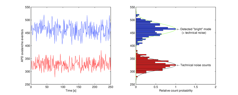
Figure 5: SPDM time series and statistical distributions for $\Phi_{A}\sim 2\times 10^{7}$ photons/sec.

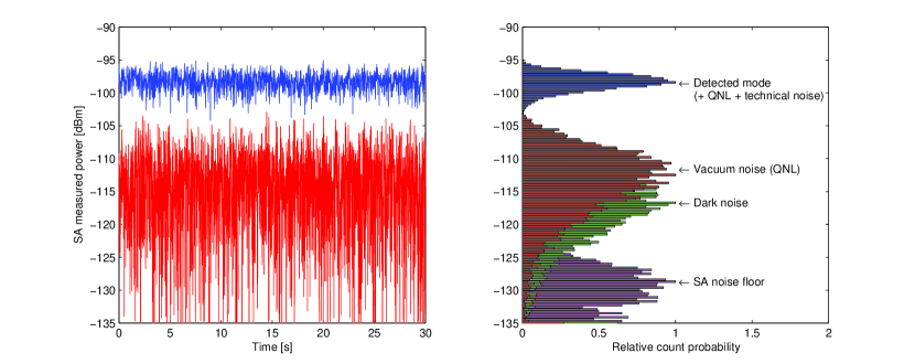
Figure 6: Homodyne detector time series and statistical distributions for $\Phi_{A}\sim 2\times 10^{7}$ photons/sec. For clarity, only the distributions associated with the technical noise sources are illustrated.

Other than the obvious differences in dynamic range, the demonstrated homodyne measurement technique differs from the SPDM photon-counting approach in a number of other aspects.

Most significantly, the homodyne detector is a continuous variable measurement system, and thus is unsuitable for conditioning purposes, such as required by non-deterministic qubit operations for implementation of linear optical quantum computation KLM .

Homodyne detection is also inherently sensitive to the spatial mode, polarisation and frequency of the input state to be measured. The RBW of the SA dictates the frequency selectivity of the technique, with the maximum detection bandwidth determined by the RF components, i.e. the linear photodetectors, subtractor and SA. As detection is reliant on optical inference at the beamsplitter, the spatial and polarisation mode of the LO and signal beams must be identical. This provides a high degree of immunity to the detection of ambient light as such photons are incoherent with either the signal or LO.

Conversely, the SPDM is insensitive to the input spatial mode, and exhibits frequency sensitivity only in response to the bandwidth of the input optics and the spectral responsivity of the semiconductor APD. Experimentally, this gave rise to two sources of systematic error; the coupling of ambient room light to fiber cladding modes which could be controlled by shielding the SPDM SMF input, and that due to the AOM isotropically scattering a portion of the (unshifted) input beam and this light being modematched into the SMF. Reducing the AOM optical input power by changing the preceding beamsplitter ratio reduced the count rates arising from this effect to a level comparable to the APD dark count rate.

Technical noise adversely affects both measurement schemes. In the SPDM, technical noise manifests itself as undesired count events and missed detection events, these effects becoming dominant at low flux levels. This is primarily a consequence of low quantum efficiency and dark counts, both of these a function of the APD semiconductor material. The time series for the SPDM shown in Fig. 5 illustrates typical data when the SPDM is illuminated (upper trace) and in the absence of optical input (lower trace). The probability density function of the ”bright” data is given by Eqn. 4 and the distribution for the dark counts is also Poissonian in nature Xiaoli92 . As both distributions are of the same family, the mean of the technical noise may simply be subtracted away Agilent1303 to yield the mean number of detection events, provided that the two distributions may be resolved.

In the homodyne scheme, technical noise is comprised mainly of electronic noise, the primary sources being the SA noise floor and dark noise from the detectors, i.e. noise generated in the absence of optical input. The time series data and associated log-Rician HillSA90 ; Agilent1303 distributions for these sources are shown in Fig. 6, along with the detected quantum noise limit (QNL) and desired signal. Although, as above, the contribution of dark noise may be subtracted away from the measured QNL, the noise serves to decrease the precision of the measurement. This deleterious effect may thus be minimised by increasing the separation between the observed QNL and the technical noise. As the detector photocurrent linearly scales with the optical input intensity within limits imposed by saturation BachorRalph , the increase in signal to technical noise ratio may be readily achieved by raising the local oscillator power.

The statistical uncertainty in each measurement $\sigma_{m}^{2}\propto N^{-1}$ where $N$ is the number of independent sample points considered Bevington . As $\sigma_{m}^{2}$ dominates the final uncertainty in $\Phi$, the measurement precision may be improved by increasing $N$ within practical time constraints. As demonstrated, the homodyne detector permits much larger values of $N$ to be attained whilst the total integration time $N\tau$ = 30 s remains small compared to 250 s for the SPDM.

VI Conclusion

We have experimentally verified the proposed homodyne measurement technique and demonstrated a superior sensitivity, dynamic range and measurement speed than is otherwise possible via linear PIN photodetectors or APD based SPDMs. The homodyne detection scheme also offers intrinsic polarisation, spatial and frequency selectivity, and does not require elaborate phase locking.

The results of simultaneous quadrature and APD measurements also clearly differentiate between semi-classical and fully quantum models of optics. In particular, semiclassical models such as stochastic electrodynamics MarshallPRA90 are unable to account for the observed quadrature variance at the QNL in the absence of photon detection events of the SPDM TCRprl00 .

- (1) D. F. Walls and G. J. Milburn. Quantum Optics. Springer-Verlag, Berlin, 1995.
- (2) G. Zambra, A. Andreoni, M. Bondani, M. Gramegna, M. Genovese, G. Brida, A. Rossi, and M. G. A. Paris. Experimental reconstruction of photon statistics without photon counting. Phys. Rev. Lett., 95, 063602, (2005).
- (3) H-A. Bachor and T. C. Ralph. A Guide to Experiments in Quantum Optics. Wiley-VCH, Weinheim, 2nd edition, 2004.
- (4) C. M. Caves and K. Wódkiewicz. Classical phase-space descriptions of continuous-variable teleportation. Phys. Rev. Lett., 93, 040506, (2004).
- (5) R. T. Thew, K. Nemoto, A. G. White, and W. J. Munro. Qudit quantum-state tomography. Phys. Rev. A, 66, 012303, (2002).
- (6) E. H. Huntington, G. N. Milford, C. Robilliard, T. C. Ralph, O. Glöckl, U. L. Andersen, S. Lorenz, and G. Leuchs. Demonstration of the spatial separation of the entangled quantum sidebands of an optical field. Phys. Rev. A, 71, 041802(R), (2005).
- (7) T. C. Ralph, W. J. Munro, and R. E. S. Polkinghorne. Proposal for the measurement of Bell-type correlations from continuous variables. Phys. Rev. Lett., 85, 10:2035–2039, (2000).
- (8) A. Korpel. Acousto-optics - a review of fundamentals. Proceedings of the IEEE, 69(1):48–53, January 1981.
- (9) B. A. E. Saleh and M. C. Teich. Fundamentals of Photonics. Wiley, New York, 1991.
- (10) E. H. Young and S-K. Yao. Design considerations for acousto-optic devices. Proceedings of the IEEE, 69(1):54–64, January 1981.
- (11) D. Stucki, G. Ribordy, A. Stefanov, H. Zbinden, J. G. Rarity, and T. Wall. Photon counting for quantum key distribution with Peltier cooled InGaAs/InP APDs. J. Mod. Optics, 48(13):1967–1981, (2001).
- (12) E. Knill, L. Laflamme, and G. J. Milburn. Efficient linear optics quantum computation. Nature, 409(46), 2001.
- (13) X. Sun and F. M. Davidson. Photon counting with silicon avalanche photodiodes. Journ. Lightwave Tech., 10(8):1023–1032, August 1992.
- (14) Spectrum analyzer measurements and noise. Technical Report 5966-4008E, Agilent Technologies, 2003.
- (15) D. A. Hill and D. P. Haworth. Accurate measurement of low signal-to-noise ratios using a superheterodyne spectrum analyser. IEEE Transactions on Instrumentation and Measurement, 39(2):432–435, April 1990.
- (16) P. R. Bevington and D. K. Robinson. Data Reduction and Error Analysis for the Physical Sciences. WCB/Mc-Graw Hill, 2nd edition, 1992.
- (17) T. W. Marshall and E. Santos. Langevin equation for the squeezing of light by means of a parametric oscillator. Phys. Rev. A, 41(3):1582-1586, (1990).