Symmetric measurements attaining the accessible information

Abstract

A theorem of Davies states that for symmetric quantum states there exists a symmetric POVM maximizing the mutual information. To apply this theorem the representation of the symmetry group has to be irreducible. We obtain a similar yet weaker result for reducible representations. We apply our results to the double trines ensemble and show numerically that for this ensemble the pretty good measurement is optimal.

1 Introduction

One of the basic problems of quantum information theory is the quantum detection problem: Given an unknown element of a finite set of possible states we want to obtain as much knowledge as possible about this state by performing measurements. More precisely, we look for a positive operator-valued measure (POVM) that minimizes or maximizes a certain optimality criterion. There are different criteria for the detection of quantum states. For example, we can consider the detection error probability, Bayes costs [1], or the mutual information [2, 3]. In this article we only consider the mutual information of a measurement.

Compared to other criteria the mutual information leads to very hard optimization problems even for simple state sets. This is due to the logarithm in the definition of the mutual information whereas other criteria as the error probability or Bayes costs are much simpler. There is only little known about optimal measurements for the mutual information [2, 3, 4, 5, 6]. The principal idea for obtaining these results is to use the convex structure of the POVMs and the mutual information. Standard arguments for convex functions and sets [7, 8, 9], e.g., Carathéodory’s theorem, can be applied. Davies showed with these arguments that we can find optimal measurements with a certain number of POVM operators [2]. Furthermore, for symmetric state sets there exists an optimal measurement whose POVM operators constitute a single orbit. The proof of this theorem only works for irreducible representations of the symmetry group and the theorem cannot be generalized directly to reducible representations as the example of Refs. [4, 5] shows. This means that for certain state sets with a reducible representation of the symmetry group it is not possible to obtain an optimal POVM which is a single orbit.

In this article we generalize Davies’ theorem to reducible representations. The generalization states that there is an optimal symmetric POVM where we know an upper bound for the number of orbits. The upper bound depends on the number of irreducible components in the representation of the symmetry group. We apply the generalization to the double trine ensemble and show numerically that the pretty good measurement of Refs. [6, 10] is an optimal measurement for this state set.

We proceed as follows. In the next two sections we recapitulate basic definitions and properties of POVMs, symmetric matrices, and the mutual information. In Sec. 4 we show how both of Davies’ theorems can be proved with a theorem that directly follows from the theory of convex sets. This theorem leads to the generalization to reducible representations. In Sec. 5 we apply the generalized theorem to two special cases of the lifted trines.

2 Symmetric states, POVMs, and matrices

In this section we outline basic definitions of symmetric quantum states and POVMs. We show that the symmetry of POVMs naturally leads to matrices with symmetry.

2.1 Symmetric states and POVMs

We consider a quantum system with corresponding Hilbert space ${\mathbbm{C}}^{d}$. A state of the system can be described by a density matrix $\rho\in{\mathbbm{C}}^{d\times d}$, i.e., a semi-positive matrix with ${\rm tr}(\rho)=1$. In the following we refer to a state set $S=\{\rho_{1},\ldots,\rho_{m}\}$ with corresponding prior probabilities $p(i)$ as an ensemble. A pure state $\rho_{i}=|\Psi_{i}\rangle\langle\Psi_{i}|$ can be described by the state vector $|\Psi_{i}\rangle$. A POVM measurement is defined by a set $P=\{\Pi_{1},\ldots,\Pi_{n}\}\subseteq{\mathbbm{C}}^{d\times d}$ of non-zero semi-positive matrices with $\sum_{i}\Pi_{i}=I_{d}$ where $I_{d}$ denotes the identity matrix of size $d\times d$. The result of a measurement is an index $i$ which occurs with the probability ${\rm tr}(\Pi_{i}\rho)$ when $\rho$ is the given state.

The symmetry of ensembles and POVMs is defined by the invariance of the corresponding set of matrices under the action of a group.

Definition 1.

Let $X=\{X_{1},\ldots,X_{m}\}\subseteq{\mathbbm{C}}^{d\times d}$ be the set of matrices corresponding to a POVM or ensemble. Furthermore, let $G$ be a finite group with unitary representation $\sigma:G\to{\mathbbm{C}}^{d\times d}$. The POVM or ensemble is symmetric with respect to $\sigma$ if $X$ is invariant under the operation $X_{i}\mapsto\sigma(g)X_{i}\sigma(g)^{\dagger}$ for all $g\in G$ and $i\in\{1,\ldots,m\}$, i.e., this operation defines a permutation representation on $X$. For ensembles we additionally assume equal prior probabilities for states of the same orbit.

Following this definition, we assume that $\sigma$ is a non-projective representation. As discussed in Ref. [11], a projective representation can be transformed into a non-projective representation by a central extension of $G$. Furthermore, we do not assume that $G$ operates transitively on $X$. This allows that we can consider the symmetries that are defined by the subgroups of $G$, too. In particular, the group $G$ can be the trivial group.

An important construction for POVMs is the symmetrization. This means that a POVM can be extended to a symmetric POVM as the following lemma states [2]. The symmetric POVM can contain several orbits and the matrices need not be distinct.

Lemma 2.

Let $P\subseteq{\mathbbm{C}}^{d\times d}$ be a POVM and $\sigma:G\to{\mathbbm{C}}^{d\times d}$ a unitary representation of the finite group $G$. Then

$$P^{G}:=\left\{\frac{1}{|G|}\sigma(g)\Pi\sigma(g)^{\dagger}:g\in G,\Pi\in P\right\}$$

is a symmetric POVM.

Another construction to obtain new POVMs is the convex combination:

Definition 3.

Let $P=\{\Pi_{1},\ldots,\Pi_{m}\}$ and ${\tilde{P}}=\{{\tilde{\Pi}}_{1},\ldots,{\tilde{\Pi}}_{n}\}$ be two POVMs of a system. For $\lambda\in[0,1]$ define the convex combination

$$\lambda P+(1-\lambda){\tilde{P}}:=\{\lambda\Pi_{1},\ldots,\lambda\Pi_{m},(1-\lambda){\tilde{\Pi}}_{1},\ldots,(1-\lambda){\tilde{\Pi}}_{n}\}.$$

This convex combination corresponds to a random selection between two POVMs. We do not forget which POVM we have chosen after the measurement, i.e., we assume that the results of both POVMs are distinct.

2.2 Matrices with symmetry

The matrices of a POVM are Hermitian. The $d^{2}$ matrices

$$E_{kk}:=|k\rangle\langle k|,\;X_{kl}:=|k\rangle\langle l|+|l\rangle\langle k|,\;{\rm and}\;Y_{kl}:=i|k\rangle\langle l|-i|l\rangle\langle k|,$$ (1)

$k>l$, of size $(d\times d)$ constitute an orthogonal basis for the real linear space of Hermitian matrices with the trace inner product. For symmetric POVMs we construct specific matrices in subspaces that can be described by the theory of symmetric matrices [12].

Definition 4.

Let $G$ be a finite group with representations $\sigma:G\to{\mathbbm{C}}^{m\times m}$ and $\tau:G\to{\mathbbm{C}}^{n\times n}$. The matrix $M\in{\mathbbm{C}}^{m\times n}$ has the symmetry $(G,\sigma,\tau)$ if $\sigma(g)M=M\tau(g)$ for all $g\in G$. We write $\sigma M=M\tau$.

Due to Schur’s lemma [13] a symmetric matrix has a special structure which can be described with the intertwining space [15] of two representations.

Definition 5.

Let $G,\sigma$ and $\tau$ be as in Def. 4. The intertwining space of $\sigma$ and $\tau$ is the linear space ${\rm Int}(\sigma,\tau):=\{M\in{\mathbbm{C}}^{m\times n}:\sigma M=M\tau\}$.

A matrix $M$ has the symmetry $(G,\sigma,\tau)$ if and only if $M\in{\rm Int}(\sigma,\tau)$. Hence, the structure of a symmetric matrix is determined by the structure of the intertwining space. The latter can be easily described if we assume that

$$\sigma=\bigoplus_{i=1}^{z}(I_{m_{i}}\otimes\kappa_{i})\quad{\rm and}\quad\tau=\bigoplus_{i=1}^{z}(I_{n_{i}}\otimes\kappa_{i})$$ (2)

are decompositions of $\sigma$ and $\tau$ into the irreducible representations $\kappa_{i}$ of $G$. These decompositions can be obtained by conjugation of $\sigma$ and $\tau$ with appropriate unitary matrices [13]. The natural numbers $m_{i}$ and $n_{i}$ are the multiplicities [14] of the irreducible representations $\kappa_{i}$ in $\sigma$ and $\tau$. The following lemma specifies the structure of the intertwining space [15].

Lemma 6.

Let $\sigma$ and $\tau$ be two representations of $G$ with the decompositions of Eq. (2). Then

$${\rm Int}(\sigma,\tau)=({\mathbbm{C}}^{m_{1}\times n_{1}}\otimes I_{{\rm deg}(\kappa_{1})})\oplus\ldots\oplus({\mathbbm{C}}^{m_{z}\times n_{z}}\otimes I_{{\rm deg}(\kappa_{z})})$$

where ${\rm deg}(\kappa_{i})$ denotes the degree of $\kappa_{i}$.

For $m_{i}=0$ we insert $n_{i}\,{\rm deg}(\kappa_{i})$ zero columns and for $n_{i}=0$ we insert $m_{i}\,{\rm deg}(\kappa_{i})$ zero rows at the appropriate positions. For symmetric ensembles and POVMs we only need a special case of this lemma. Let $X_{i}$ be symmetric states or POVM operators. Then $C:=\sum_{i}X_{i}$ is invariant under the conjugation with $\sigma$, i.e.,

$$\sigma(g)C\sigma(g)^{\dagger}=C\quad\hbox{for all}\quad g\in G.$$

This means, that $\sigma C=C\sigma$. Using Lemma 6 we see that $C$ is a Hermitian block-diagonal matrix with blocks that are Hermitian matrices, too. The following lemma determines the dimension of the intertwining space.

Lemma 7.

Let $\sigma$ be as in Eq. (2). Then the Hermitian matrices in ${\rm Int}(\sigma,\sigma)$ constitute a linear space of real dimension $\sum_{i}m_{i}^{2}$.

Assume that $\sigma$ is irreducible. Then ${\rm Int}(\sigma,\sigma)$ is an one-dimensional space since it contains only real scalar multiples of the identity matrix. For a representation of the trivial group ${\rm Int}(\sigma,\sigma)$ is the full space of matrices, i.e., the linear space has the dimension $d^{2}$.

3 Basic properties of mutual information

Let $S$ be an ensemble and $P$ be a POVM as defined in Sec. 2.1. Using the conditional probability $p(j|i):={\rm tr}(\Pi_{j}\rho_{i})$ we can define the joint probability distribution $p_{ij}:=p(i)p(j|i)$. With this distribution we can define the mutual information as in classical information theory [16].

Definition 8.

The mutual information of the ensemble $S$ and POVM $P$ is

$$I(S,P):=\sum_{i=1}^{m}\sum_{j=1}^{n}H(p_{ij})-\sum_{i=1}^{m}H\left(\sum_{j=1}^{n}p_{ij}\right)-\sum_{j=1}^{n}H\left(\sum_{i=1}^{m}p_{ij}\right)$$ (3)

with $H(u)=u\,{\rm log}_{2}\,u$.

The fundamental problem is to find a POVM $P$ that maximizes $I(S,P)$ for a given ensemble $S$ with prior probabilities $p(i)$. The information obtained by an optimal measurement is called the accessible information [3].

We resume some properties of the mutual information which can be used to transform optimal measurements into a normal form. Then the optimization can be restricted to these POVMs. The first lemma directly follows from classical information theory (see Th. 2.7.4 in Ref. [16]) and essentially states that the mutual information is a convex function in the conditional probability $p(j|i)$ for a fixed distribution $p(i)$.

Lemma 9.

Let $P=\{\Pi_{1},\ldots,\Pi_{n}\}$ as well as ${\tilde{P}}=\{{\tilde{\Pi}}_{1},\ldots,{\tilde{\Pi}}_{n}\}$ be POVMs and $S$ an ensemble. Define the POVM $Q:=\{\lambda\Pi_{i}+(1-\lambda){\tilde{\Pi}}_{i}:i=1,\ldots,n\}$ for $\lambda\in[0,1]$. Then the inequality

$$I(S,Q)\leq\lambda I(S,P)+(1-\lambda)I(S,{\tilde{P}})$$

holds. The equality holds if and only if

$$p_{ij}\sum_{k}{\tilde{p}}_{kj}={\tilde{p}}_{ij}\sum_{k}p_{kj}$$

for all $i$ and $j$ where ${\tilde{p}}_{ij}:=p(i){\rm tr}({\tilde{\Pi}}_{j}\rho_{i})$.

The equality condition holds exactly for POVMs with the property that the probability vectors $(p_{1j},\ldots,p_{mj})$ and $({\tilde{p}}_{1j},\ldots,{\tilde{p}}_{mj})$ that are induced by $\Pi_{j}$ and ${\tilde{\Pi}}_{j}$ for the given ensemble are equal up to a constant factor:

$$c_{j}(p_{1j},\ldots,p_{mj})=d_{j}({\tilde{p}}_{1j},\ldots,{\tilde{p}}_{mj})$$

for $c_{j},d_{j}\geq 0$ with $c_{j}+d_{j}>0$ for each $j$. In other words, for the given ensemble both operators are indistinguishable up to the constant factor.

The convex combination of POVMs in Lemma 9 differs from Def. 3. We obtain the latter by padding $P$ from the right and ${\tilde{P}}$ from the left with zero operators in such a way that all combinations $\lambda\Pi_{i}+(1-\lambda){\tilde{\Pi}}_{i}$ encompass one zero operator. Then we have $\sum_{k}p_{kj}=0$ or $\sum_{k}{\tilde{p}}_{kj}=0$ for all $j$, i.e., we have $c_{j}=0$ or $d_{j}=0$. Consequently, the information obtained by the convex combination of two POVMs is the convex combination of the corresponding informations:

Lemma 10.

Let $S$ be an ensemble and let $P$ as well as ${\tilde{P}}$ be POVMs. Then for all $\lambda\in[0,1]$ the equality

$$I(S,\lambda P+(1-\lambda){\tilde{P}})=\lambda I(S,P)+(1-\lambda)I(S,{\tilde{P}})$$

holds.

This lemma has a simple interpretation: For measurements we randomly choose between two devices. Then the total information we obtain is the weighted average of the informations for each device.

The next lemma (see Lemma 2 of Ref. [2]) shows that POVM operators that are equal up to normalization can be merged without changing the mutual information of the POVM. The same is true if we split an operator $\Pi_{i}$ into $\lambda\Pi_{i}$ and $(1-\lambda)\Pi_{i}$ for $0\leq\lambda\leq 1$. This theorem can be applied repeatedly and to permutations of the operators, too.

Lemma 11.

Let $S$ be an ensemble. Then $I(S,{\tilde{P}})=I(S,P)$ holds for the POVMs $P=\{\Pi_{1},\Pi_{2},\ldots,\Pi_{n}\}$ and ${\tilde{P}}=\{\lambda\Pi_{1},(1-\lambda)\Pi_{1},\Pi_{2},\Pi_{3},\ldots,\Pi_{n}\}$ with $0\leq\lambda\leq 1$.

The optimization of POVMs can be simplified in some cases if we use a special normalization of the POVM operators. The following definition shows how a POVM can be rewritten in such a way that the resolution $\sum_{i}\Pi_{i}=I_{d}$ of the identity is a convex combination [2].

Definition 12.

Let $P=\{\Pi_{1},\ldots,\Pi_{n}\}$ be a POVM with non-zero operators. Then write $P=\{\lambda_{1}\Pi_{1}^{\prime},\ldots,\lambda_{n}\Pi_{n}^{\prime}\}$ with

$$\Pi_{i}^{\prime}:=\frac{d}{{\rm tr}(\Pi_{i})}\Pi_{i}\quad{\rm and}\quad\lambda_{i}:=\frac{{\rm tr}(\Pi_{i})}{d}.$$

The identity is the convex combination $\sum_{i}\lambda_{i}\Pi_{i}^{\prime}=I_{d}$.

The last lemma of this section is a generalization of Lemma 5 in Ref. [2] and can be applied to symmetric ensembles. It states that for a given POVM the symmetrization of this POVM has the same mutual information. Hence, we know that for symmetric ensembles there always exists an optimal symmetric POVM. In the next section we prove the existence of a symmetric POVM where we know an upper bound for the number of orbits.

Lemma 13.

Let $S$ be a symmetric ensemble with symmetry group $G$ and let $P$ be a POVM. Then $I(S,P)=I(S,P^{G})$.

To apply this theorem the symmetry group need not operate transitively on the ensemble. The probabilities $p(i)$ have to be constant on each orbit.

4 Optimal POVMs for symmetric ensembles

In the literature, the main tools for the optimization of POVMs are Davies’ theorems [2] and their real versions [3]. We briefly recapitulate the proofs and generalize the theorem for symmetric ensembles to reducible representations of the symmetry group.

Davies’ first theorem (Th. 3 of Ref. [2]) states that for an ensemble of a $d$-dimensional Hilbert space there exists an optimal POVM with $n$ rank-one operators where $d\leq n\leq d^{2}$. Davies’ proof is essentially based on the following lemma which deals with convex combinations of the identity. The set of these combinations is convex and the lemma gives an upper bound for the number of operators of an extreme point [2]. We prove this lemma in the appendix with standard arguments of linear optimization.

Lemma 14.

Let $\sum_{i}\lambda_{i}\Pi_{i}^{\prime}=I_{d}$ be a convex combination with ${\rm tr}(\Pi_{i}^{\prime})=d$. Furthermore, let all $\Pi_{i}^{\prime}$ be elements of the affine space $I_{d}+K$ where $K$ is an $r$-dimensional linear subspace of Hermitian matrices. Then the convex combination can be rewritten as

$$\sum_{i}\lambda_{i}\Pi_{i}^{\prime}=\sum_{i}\mu_{i}\left(\sum_{j}\nu_{ij}\Pi_{j}^{\prime}\right)\;{\rm with}\;\sum_{j}\nu_{ij}\Pi_{j}^{\prime}=I_{d}$$

where $\mu_{i},\nu_{ij}\geq 0$ and $\sum_{j}\mu_{j}=\sum_{j}\nu_{ij}=1$ for all $i$. Furthermore, for each $i$ at most $r+1$ elements $\nu_{ij}$ are non-zero.

Using this lemma we can prove the upper bound of Davies’ first theorem as follows. Assume that $\Pi_{1},\ldots,\Pi_{n}$ is an optimal POVM. We can assume that it consists of rank-one operators [2]. Using the normalization of Def. 12 we have a convex combination $\sum_{i}\lambda_{i}\Pi_{i}^{\prime}=I_{d}$. With Lemma 14 the POVM is a convex combination of POVMs with at most $d^{2}$ operators each because $K$ has dimension $d^{2}-1$. Lemmas 10 and 11 show that at least one of these POVMs is optimal, too.

We show how Davies’ second theorem (Th. 4 of Ref. [2]) follows from Lemma 14. The former states that for a symmetric ensemble with irreducible representation $\sigma$ there exists an optimal POVM which is a single orbit. Let $P$ be an optimal POVM with rank-one operators. Following Lemma 13 the POVM $P^{G}$ is optimal, too. We consider the orbits

$$C_{i}:=\left\{\frac{1}{|G|}\sigma(g)\Pi_{i}^{\prime}\sigma(g)^{\dagger}:g\in G\right\}$$

of the operators of $P$. We have the convex combination $\sum_{i}\lambda_{i}C_{i}=P^{G}$ with $\lambda_{i}:={\rm tr}(\Pi_{i})/d$ as in Def. 12. We consider the orbit sums

$$D_{i}:=\frac{1}{|G|}\sum_{g\in G}\sigma(g)\Pi_{i}^{\prime}\sigma(g)^{\dagger}.$$

Since $P^{G}$ is a POVM the equation $\sum_{i}\lambda_{i}D_{i}=I_{d}$ holds, i.e., the identity matrix is a convex combination of the matrices $D_{i}$. We use the irreducibility of $\sigma$ and obtain due to $\sigma D_{i}=D_{i}\sigma$ the equation $D_{i}=I_{d}$. In other words, the matrices $D_{i}$ are elements of the intertwining space ${\rm Int}(\sigma,\sigma)={\mathbbm{C}}I_{d}$. Since the matrices $D_{i}$ have trace $d$ they are elements of the affine space $I_{d}+\{0\}$ whose real dimension is $r=0$. Following Lemma 14 there exists a convex combination of $I_{d}$ with a single $D_{i}$. With the same arguments as for the proof of Davies’ first theorem a single orbit is sufficient for an optimal measurement.

It is clear how this proof of Davies’ second theorem is modified for reducible representations: The matrices $D_{i}$ are elements of the intertwining space ${\rm Int}(\sigma,\sigma)$ which has dimension $r:=\sum_{i}m_{i}^{2}$ as stated in Lemma 7. The trace normalization reduces the dimension by one. Then Lemma 14 states that we need at most $r$ orbits to construct the identity matrix. The preceding discussion shows the following theorem.

Theorem 15.

Let $S$ be a symmetric ensemble with $\sigma$ as defined in Eq. (2). Then there exists an optimal measurement with rank-one operators which is the union of at most $\sum_{i}m_{i}^{2}$ orbits.

The theorem can also be applied if we restrict the symmetry to subgroups of the symmetry group since the action of the group must not be transitive. However, by this reduction the bound on the number of orbits becomes weaker since the number of different irreducible representations decreases while the multiplicities $m_{i}$ increase. Therefore, for the solution of optimization problems it is beneficial to take as much symmetry as possible. As an extreme case, this theorem can be applied to a representation of the trivial group. Then we have $m_{1}=d$ for the only irreducible representation $g\mapsto(1)$ leading to the upper bound $d^{2}$. This discussion shows that Davies’ first theorem can be obtained as special case of the generalized theorem.

Both theorems have real versions [3]. The bound of the first theorem can be tightened to $n\leq d(d+1)/2$ since we can transform an optimal POVM into a POVM with real operators. Hence, the subspace $K$ of Lemma 14 does not contain linear combinations of the elements $Y_{kl}$ of Eq. (1). Additionally, the discussion for the second theorem is also valid if we replace the $\kappa_{i}$ of Eq. (2) with the real irreducible representations. We obtain the upper bound $\sum_{i}m_{i}(m_{i}+1)/2$ where the $m_{i}$ are the multiplicities of the real irreducible representations.

5 Examples

We apply the real version of Th. 15 to the following ensembles in order to obtain optimal POVMs: an ensemble of slightly lifted trines and the double trines. The theorem leads to an optimization problem that is a special case of those in Refs. [4, 5]. We identify optimal POVMs and discuss their properties. For the slightly lifted trines we conclude as in Refs. [4, 5] that a symmetric optimal POVM must at least comprise two orbits. For the double trines we obtain an optimal POVM consisting of a single orbit.

5.1 Lifted trines

For each $\alpha\in[0,1]$ the three vectors

$$\left(\begin{array}[]{c}\sqrt{\alpha}\\ \sqrt{1-\alpha}\\ 0\\ \end{array}\right),\left(\begin{array}[]{c}\sqrt{\alpha}\\ -\frac{1}{2}\sqrt{1-\alpha}\\ \frac{\sqrt{3}}{2}\sqrt{1-\alpha}\end{array}\right),\;{\rm and}\;\left(\begin{array}[]{c}\sqrt{\alpha}\\ -\frac{1}{2}\sqrt{1-\alpha}\\ -\frac{\sqrt{3}}{2}\sqrt{1-\alpha}\end{array}\right)$$

constitute a lifted trines ensemble. These ensembles are interesting since for slightly lifted trines, i.e., $\alpha$ is next to zero, it can be numerically shown that two orbits are necessary to obtain an optimal POVM [4, 5]. This shows that the direct generalization of Davies’ theorem to reducible representations is not possible and that the bound of Th. 15 can be attained.

We follow Refs. [4, 5] and show in detail the analysis of optimal measurements for a special case of the lifted trines. The symmetry group of the lifted trines is generated by the rotation

$$R:=\frac{1}{2}\left(\begin{array}[]{ccc}2&0&0\\ 0&-1&\sqrt{3}\\ 0&-\sqrt{3}&-1\end{array}\right)$$

about $120$ degrees. This representation of the symmetry group contains two inequivalent real irreducible representations. Each irreducible representation has the multiplicity one. Hence, using the real version of Th. 15 we need at most two orbits $C_{1}=\{\Pi,R\Pi R^{2},R^{2}\Pi R\}$ and $C_{2}=\{{\tilde{\Pi}},R{\tilde{\Pi}}R^{2},R^{2}{\tilde{\Pi}}R\}$ with operators $\Pi$ and ${\tilde{\Pi}}$ of rank one to obtain an optimal POVM. With the normalization ${\rm tr}(\Pi)={\rm tr}({\tilde{\Pi}})=1$ the convex combination $P=\lambda C_{1}+(1-\lambda)C_{2}$ is a POVM for appropriate $\Pi$, ${\tilde{\Pi}}$, and $\lambda\in[0,1]$. We apply Lemma 10 and obtain the information $I(S,P)=\lambda I(S,C_{1})+(1-\lambda)I(S,C_{2})$, i.e., the mutual information of a convex combination of orbits is the convex combination of the formal mutual informations $I(S,C_{1})$ and $I(S,C_{2})$. For an operator $\Pi=|\Psi(a,b)\rangle\langle\Psi(a,b)|$ we use the parameterization

$$|\Psi(a,b)\rangle=\left(\begin{array}[]{c}{\rm cos}(a)\\ {\rm sin}(a){\rm cos}(b)\\ {\rm sin}(a){\rm sin}(b)\end{array}\right)$$ (4)

leading to the orbit sum

$$\sum_{i=0}^{2}R^{i}\Pi R^{-i}=\left(\begin{array}[]{ccc}3\,{\rm cos}^{2}(a)&0&0\\ 0&\frac{3}{2}-\frac{3}{2}\,{\rm cos}^{2}(a)&0\\ 0&0&\frac{3}{2}-\frac{3}{2}\,{\rm cos}^{2}(a)\end{array}\right).$$

For two orbits $C_{1}$ and $C_{2}$ with parameters $(a,b)$ and $(c,d)$ the convex combination $\lambda C_{1}+(1-\lambda)C_{2}$ is a POVM, i.e., the sum of all operators equals $I_{3}$, if and only if

$$\lambda\,{\rm cos}^{2}(a)+(1-\lambda)\,{\rm cos}^{2}(c)=\frac{1}{3}.$$ (5)

If we assume ${\rm cos}^{2}(a)\leq{\rm cos}^{2}(c)$ this means that $1/3\in[{\rm cos}^{2}(a),{\rm cos}^{2}(c)]$, i.e., ${\rm cos}^{2}(a)\in[0,1/3]$ and ${\rm cos}^{2}(c)\in[1/3,1]$ are all possible values. In the following we only consider the mutual information $I(a,b)$ of the orbit with $a={\rm arccos}\sqrt{x}$, $x\in[0,1]$, and $b\in[0,2\pi/3]$. This is sufficient since for a given value ${\rm cos}(a)$ with ${\rm cos}^{2}(a)=x$ we have the four possible values ${\rm cos}(a)=\pm\sqrt{x}$ and ${\rm sin}(a)=\pm\sqrt{1-x}$ in the vector $|\Psi(a,b)\rangle$ of Eq. (4). We denote these combinations of signs by $++$, $+-$, $-+$, and $--$. The case $--$ leads to the same information as $++$ since the corresponding vectors differ only by a global phase. With the same argument the cases $-+$ and $+-$ lead to the same mutual information. For $+-$ the vector has a minus sign in the last two components. Hence, we have the same information as for $++$ where we replace $b$ by $b+\pi$. This discussion shows that the optimization with $({\rm arccos}\sqrt{x},b)$ for $x\in[0,1]$ and $b\in[0,2\pi/3]$ takes all possible values into account.

We restrict our attention to $\alpha=1/20$, i.e., to an example of slightly lifted trines. In Figs. 1 and 2

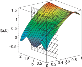
Figure 1: The mutual information $I({\rm arccos}\sqrt{x},b)$ for the lifted trines with $\alpha=1/20$. The information of an orbit can be negative. However, as Fig. 2 shows the convex combination of the information of two points on different sides of the plane $x=1/3$ leads to a non-negative information.

the information $I({\rm arccos}\sqrt{x},b)$ of an orbit with parameters $({\rm arccos}\sqrt{x},b)$ is shown. Due to the symmetry each probability $p_{ij}$ is equal to the probability $p_{1k}$ for a certain $k$.

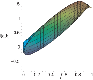
Figure 2: Fig. 1 viewed along the $b$-axis shows the maximum of $I({\rm arccos}\sqrt{x},b)$ for each $x$ whereas $b$ remains a variable. This maximum is slightly convex in the interval $[0,0.3831]$ of the $x$-axis.

Hence, the information of the orbit is

$$I({\rm arccos}\sqrt{x},b)=3(H(p_{11})+H(p_{12})+H(p_{13})-H(p_{11}+p_{12}+p_{13}))+{\rm log}_{2}3.$$

The condition of Eq. (5) means that

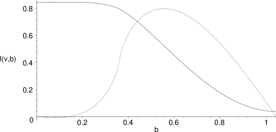
Figure 3: The function $I(\nu,b)$ has a global maximum at $b\approx 0.1377$. It seems to be complicated to give a simple analytic definition of this value. The partially negative function is $-(d/db)I(\nu,b)/2$. The remaining values can be obtained by virtue of the symmetry of the function.

the points $(a,b)$ and $(c,d)$ we choose for our orbits lie on different sides of the plane $x=1/3$. From the figures it follows that a single orbit cannot be optimal since a POVM with a single orbit corresponds to a point on this plane. More precisely, the optimal information we can obtain for points on this plane is $0.8456$ bit as shown in Fig. 3. This can be obtained for the POVM with $(\nu,b)$ where $\nu:={\rm arccos}\sqrt{1/3}$ and $b\approx 0.1377$. The slight convexity in Fig. 2 as well as Refs. [4, 5] suggest that we can obtain more information with two points: a point with $x=0$ and a point with $b=0$ on the other side of the plane. Numerical computations show that an optimal point for $x=0$ is $(\pi/2,\pi/2)$ with the information $0.15996$ bit. The other optimal point can be chosen to be $(\arccos\sqrt{0.3831},0)$ with $0.9499$ bit. The convex combination of both informations is $0.8472$ bit. This is more than the information of the optimal single orbit.

In the following we show that the accessible information cannot be obtained with a POVM which is a single orbit even if we consider operators of higher rank. Consequently, the characterization [17, 18] of the extreme points of the convex set of POVMs consisting of a single orbit cannot be applied. Assume that $P:=\{R^{i}\Pi R^{-i}:i=0,1,2\}$ is an optimal POVM with initial operator $\Pi=\sum_{i=1}^{3}s_{i}|\Psi_{i}\rangle\langle\Psi_{i}|$ where $\langle\Psi_{i}|\Psi_{i}\rangle=1$, $\sum_{i}s_{i}=1$, and $s_{i}\geq 0$. Then Lemma 2 of Ref. [2] and Lemma 10 state that

$$I(S,P)\leq\sum_{i}s_{i}I(S,P_{i})=I(S,\sum_{i}s_{i}P_{i})$$ (6)

with $P_{i}:=\{R^{j}|\Psi_{i}\rangle\langle\Psi_{i}|R^{-j}:j=0,1,2\}$. The POVM $\sum_{i}s_{i}P_{i}$ consists of three orbits. Using Th. 15 we construct an optimal POVM with two of these three orbits. Without loss of generality we assume that the orbits correspond to $|\Psi_{1}\rangle\langle\Psi_{1}|$ and $|\Psi_{2}\rangle\langle\Psi_{2}|$. The two corresponding points $(a,b)$ must be the optimal points given above. The probability vectors $(0.2375,0,0.2375)$ for $|\Psi_{1}\rangle\langle\Psi_{1}|$ and $(0.2724,0.0199,0.0199)$ for $|\Psi_{2}\rangle\langle\Psi_{2}|$ are not equal up to a constant factor. Therefore, following Lemma 9 inequality (6) is strict, i.e., the single orbit cannot be an optimal POVM.

5.2 Double trines

The double trines [6, 10] are defined by the three state vectors

$$\left(\begin{array}[]{c}1\\ 0\end{array}\right)\otimes\left(\begin{array}[]{c}1\\ 0\end{array}\right)=\left(\begin{array}[]{cc}1\cr 0\cr 0\cr 0\end{array}\right),\;\frac{1}{2}\left(\begin{array}[]{c}-1\\ -\sqrt{3}\end{array}\right)\otimes\frac{1}{2}\left(\begin{array}[]{c}-1\\ -\sqrt{3}\end{array}\right)=\frac{1}{4}\left(\begin{array}[]{cc}1\cr\sqrt{3}\cr\sqrt{3}\cr 3\end{array}\right)$$

$$\;{\rm and}\;\;\frac{1}{2}\left(\begin{array}[]{c}-1\\ \sqrt{3}\end{array}\right)\otimes\frac{1}{2}\left(\begin{array}[]{c}-1\\ \sqrt{3}\end{array}\right)=\frac{1}{4}\left(\begin{array}[]{cc}1\cr-\sqrt{3}\cr-\sqrt{3}\cr 3\end{array}\right)$$

of two qubits. We apply the unitary basis transform

$$\frac{1}{\sqrt{2}}\left(\begin{array}[]{cccc}1&0&0&1\\ 1&0&0&-1\\ 0&1&1&0\\ 0&1&-1&0\end{array}\right)$$

and obtain the state vectors

$$\frac{1}{\sqrt{2}}\left(\begin{array}[]{c}1\\ 1\\ 0\\ 0\end{array}\right),\;\frac{1}{\sqrt{2}}\left(\begin{array}[]{c}1\\ -1/2\\ \sqrt{3}/2\\ 0\end{array}\right),\;{\rm and}\;\frac{1}{\sqrt{2}}\left(\begin{array}[]{c}1\\ -1/2\\ -\sqrt{3}/2\\ 0\end{array}\right).$$

We omit the last component and obtain the lifted trines with $\alpha=1/2$. In contrast to the previous section these trines are strongly lifted. As mentioned in Refs. [4, 5] this leads to different properties of optimal POVMs. We replace $\alpha=1/20$ by $\alpha=1/2$ in the computations of Sec. 5.1 and obtain Figs. 4 and 5

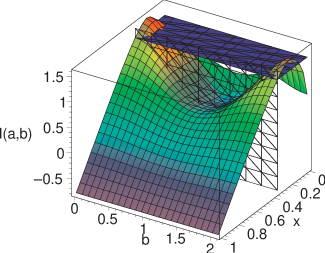
Figure 4: The mutual information $I({\rm arccos}\sqrt{x},b)$ for the double trines ensemble. The horizontal plane corresponds to the information $1.369$ bit which is the information of the pretty good measurement.

where the information $I({\rm arccos}\sqrt{x},b)$ is shown.

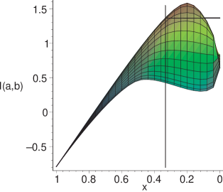
Figure 5: Fig. 4 viewed along the $b$-axis shows the maximum of $I({\rm arccos}\sqrt{x},b)$ for each $x$ whereas $b$ remains a variable.

An optimal POVM can be obtained with a convex combination of at most two orbits. It follows from Fig. 5 that a single orbit with $x=1/3$ is optimal since the convex combination of the information of two points on different sides of the plane $x=1/3$ is strictly below the maximum of the information on this plane. Computations show that $I(\nu,b)$ with $\nu={\rm arccos}\sqrt{1/3}$ has an extreme point at $b=0$. Hence, an optimal point on this plane is $(a,b)=(\nu,0)$ leading to the information

$$I(\nu,0)=\frac{2\sqrt{2}\gamma-9\,{\rm ln}(2)}{6\,{\rm ln}(2)}\approx 1.369$$

with $\gamma={\rm ln}\left(2(3+2\sqrt{2})^{2}\right)$. This is equal to the information obtained in Refs. [6, 10] for the pretty good measurement [19]. Furthermore, the Hessian

$$\left(\begin{array}[]{cc}\frac{81-27\sqrt{2}\gamma}{16\,{\rm ln}(2)}&0\\ 0&\frac{6-(2+\sqrt{2})\gamma}{3\,{\rm ln}(2)}\end{array}\right)\approx\left(\begin{array}[]{cc}-7.221&0\\ 0&-4.041\end{array}\right)$$

of $I({\rm arccos}\sqrt{x},b)$ is negative definite at the point $(x,b)=(1/3,0)$, i.e., the information is concave in this region. These arguments and the global properties of $I({\arccos}\sqrt{x},b)$ which can be seen in Figs. 4 and 5 suggest that the POVM corresponding to the point $(\nu,0)$ is optimal.

6 Conclusions

We have generalized Davies’ theorem for symmetric ensembles to reducible representations of the symmetry group. There always exists an optimal POVM consisting of at most $\sum_{i}m_{i}^{2}$ orbits where the $m_{i}$ are the multiplicities of the irreducible components in the representation of the symmetry group.

Appendix

In this appendix we prove Lemma 14 with standard arguments of linear optimization. Consider a POVM on a $d$-dimensional system with operators $\Pi_{1},\ldots,\Pi_{n}$ where we write $\Pi_{i}=\lambda_{i}\Pi_{i}^{\prime}$ as in Def. 12. We have the convex combination $\sum_{i}\lambda_{i}\Pi_{i}^{\prime}=I_{d}$. With respect to the basis of Eq. (1) this convex combination can be written as equation

$$D\lambda=\left(\begin{array}[]{c}1\\ 0\end{array}\right)\;{\rm where}\;D:=\left(\begin{array}[]{ccc}1&\ldots&1\\ &E&\\ &X&\\ &Y&\end{array}\right).$$ (7)

Here we write $\lambda=(\lambda_{1},\ldots,\lambda_{n})^{T}$. The $1$ on the right side of the equation is the all-one vector of length $d+1$ and the $0$ is the all-zero vector of length $d^{2}-d$. The matrices $E\in{\mathbbm{R}}^{d\times n}$ and $X,Y\in{\mathbbm{R}}^{((d^{2}-d)/2)\times n}$ contain the coefficients of the real linear combinations

$$\Pi_{i}=\sum_{k=0}^{d-1}\Pi_{i}^{kk}E_{kk}+\sum_{k>l}\Re(\Pi_{i}^{kl})X_{kl}+\sum_{k>l}\Im(\Pi_{i}^{kl})Y_{kl}$$

of $\Pi_{i}=(\Pi_{i}^{kl})_{kl}$ where $\Re$ and $\Im$ denote the real and imaginary part of a complex number. More precisely, the $i$-th column of $E$, $X$, and $Y$ contains the coefficients $\Pi_{i}^{kk}$, $\Re(\Pi_{i}^{kl})$, and $\Im(\Pi_{i}^{kl})$, respectively.

We discuss some elementary properties of the solutions ${\cal L}_{E}$ of $E\lambda=b$ with $\lambda_{i}\geq 0$ and the vector $b$ consisting of $d$ ones. The matrix $E$ contains only non-zero columns and non-negative entries.

Lemma 16.

The set ${\cal L}_{E}$ is convex and compact.

Proof.

The set ${\cal L}_{E}$ is closed and convex. Assume that it is unbounded. Then following Th. 2.5.1 of Ref. [7] it contains a ray, i.e., the set $\{p+\mu q:\mu\geq 0\}$ with $q\not=0$. Choose $k$ with $q_{k}\not=0$. Since we have $\lambda_{i}\geq 0$ the vector $q$ cannot contain negative entries. For all $\mu\geq 0$ we have $E(p+\mu q)=Ep+\mu Eq=b$. Hence, we have $Ep=b$ and $Eq=0$. The inequality $Eq\geq E_{k}q_{k}$ holds where $E_{k}$ denotes the $k$-th column of $E$ and $\geq$ the element-wise relation. Since $E$ does not contain a zero column we have $Eq\geq E_{k}q_{k}>0$ in contradiction to $Eq=0$. Hence, the set ${\cal L}_{E}$ cannot contain a ray. ∎

This lemma can also be applied to ${\cal L}_{D}$ since the additional equations restrict the set of solutions even more. Hence, ${\cal L}_{D}$ is convex and compact.

Lemma 17.

A compact convex subset of ${\mathbbm{R}}^{n}$ is the convex hull of its extreme points.

Proof.

See Th. 2.4.5 of Ref. [7]. ∎

Lemma 18.

The set ${\cal L}_{D}$ has only a finite number of extreme points. For an extreme point $\lambda=(\lambda_{1},\ldots,\lambda_{n})^{T}$ of ${\cal L}_{D}$ we have at most ${\rm rank}(D)$ non-zero elements $\lambda_{i}$.

Proof.

Following Th. 2.3 in Ref. [9] an extreme point of ${\cal L}_{D}$ corresponds to a feasible basic solution of $D\lambda=c$ where $c$ is the vector of Eq. (7) consisting of ones and zeros. Since the equation $\sum_{i}\lambda_{i}\Pi_{i}^{\prime}=I_{d}$ shows that ${\cal L}_{D}$ is non-empty we can remove linear dependent rows of $D$ without changing the set of solutions (see Th. 2.5 of Ref. [9]). Then Th. 2.4 of Ref. [9] states that a basic solution $\lambda$ has at most ${\rm rank}(D)$ non-zero entries. The number of extreme points is finite due to Corollary 2.1 of Ref. [9]. ∎

In the next lemma we show that ${\rm rank}(D)$ is bounded by the dimension of the space that contains all operators $\Pi_{i}^{\prime}$.

Lemma 19.

Let $\Pi_{1}^{\prime},\ldots,\Pi_{n}^{\prime}\in{\mathbbm{C}}^{d\times d}$ with ${\rm tr}(\Pi_{i}^{\prime})=d$ be elements of the affine space $I_{d}+K$ where $K$ is a $r$-dimensional linear space of Hermitian matrices. Then the matrix $D$ defined in Eq. (7) has at most rank $r+1$.

Proof.

The matrix $D$ without the first row has at most rank $r+1$ since an affine space of dimension $r$ is contained in a linear space of dimension $r+1$. The first row does not increase the rank since it is linear dependent to the rows of $E$. This is due to the normalization ${\rm tr}(\Pi_{i}^{\prime})=d$ which means that the sum of each column of $E$ is $d$. ∎

With the lemmas of this appendix we prove Lemma 14.

Proof of Lemma 14.

As in Eq. (7) we write $\sum_{i}\lambda_{i}\Pi_{i}^{\prime}=I_{d}$ as $D\lambda=c$ with the vector $c$ of Eq. (7) consisting of ones and zeros. Following Lemma 19 the matrix $D$ has at most rank $r+1$. Then Lemma 18 states that an extreme point $\lambda$ of ${\cal L}_{D}$ has at most $r+1$ non-zero elements. With Lemma 16 we know that the solutions of $D\lambda=c$ constitute a convex and compact set which is the convex combination of its extreme points as stated in Lemma 17. ∎

References

- [1] C.W. Helstrom: Quantum Detection and Estimation Theory. Academic Press, 1976.
- [2] E.B. Davies: Information and quantum measurement. IEEE Inf. Theory, IT-24, 596 (1978).
- [3] M. Sasaki, S.M. Barnett, R. Jozsa, M. Osaki, O. Hirota: Accessible information and optimal strategies for real symmetrical quantum sources. Phys. Rev. A, Vol. 59, No. 5, pp. 3325-3335, 1999.
- [4] P.W. Shor: On the Number of Elements Needed in a POVM Attaining the Accessible Information. Quantum, Communication, Measurement and Computing 3, Edited by O. Hirota and P. Tombesi, Kluwer Academic, 2001. See also quant-ph/0009077.
- [5] P.W. Shor: The Adaptive Classical Capacity of a Quantum Channel. IBM Journal of Research and Development, Vol. 48, No. 1, pp. 115-138, 2004.
- [6] A. Peres, W.K. Wootters: Optimal Detection of Quantum Information. Phys. Rev. Lett., Vol. 66, No. 9, pp. 1119-1122, 1991.
- [7] B. Grünbaum: Convex polytopes. Wiley, 1967.
- [8] E.M. Alfsen: Compact Convex Sets and Boundary Integrals. Springer, 1971.
- [9] D. Bertsimas, J.N. Tsitsiklis: Introduction to Linear Optimization. Athena Scientific, 1997.
- [10] W.K. Wootters: Distinguishing unentangled states with an unentangled measurement. quant-ph/0506149.
- [11] T. Decker, D. Janzing, M. Rötteler: Implementation of group-covariant positive operator valued measures by orthogonal measurements. J. Math. Phys. 46, 012104 (2005).
- [12] S. Egner, M. Püschel: Symmetry-Based Matrix Factorization. J. Sym. Comp., Vol. 37, No. 2, pp. 157-186, 2004.
- [13] J.-P. Serre: Linear Representations of Finite Groups. Springer, 1977.
- [14] L. Dornhoff: Group Representation Theory, Part A. Dekker, 1971.
- [15] M. Püschel: Decomposing Monomial Representations of Solvable Groups. J. Sym. Comp., Vol. 34, No. 6, pp. 561-596, 2002.
- [16] T.M. Cover, J.A. Thomas: Elements of information theory. Wiley, 1991.
- [17] G.M. D’Ariano: Extremal covariant quantum operations and positive operator valued measures. J. Math. Phys. 45, pp. 3620-3635 (2004).
- [18] G. Chiribella, G.M. D’Ariano: Extremal covariant positive operator valued measures. J. Math. Phys. 45, 4435 (2004).
- [19] P. Hausladen, W.K. Wootters: A ‘pretty good’ measurement for distinguishing quantum states. J. Mod. Opt., Vol. 41, No. 12, pp. 2385-2390, 1994.