Quantum Lubrication: Suppression of Friction in a First Principle Four Stroke Heat Engine.

Abstract

A quantum model of a heat engine resembling the Otto cycle is employed to explore strategies to suppress frictional losses. These losses are caused by the inability of the engine’s working medium to follow adiabatically the change in the Hamiltonian during the expansion and compression stages. By adding external noise to the engine frictional losses can be suppressed.

I Introduction

Working conditions of real heat engines are far from the ideal reversible limit. Their performance is restricted by irreversible losses due to heat transport, heat leaks and also friction. Actual working devices tend to optimize the performance by balancing the losses with maximizing workP. Salamon, J.D. Nulton, G. Siragusa, T.R. Andersen and A. Limon (2001). For engines producing finite power irreversible losses are unavoidable. High performance engines are therefore constructed from materials which reduce heat resistivity while minimizing heat leaks. In addition lubricants are employed to reduce frictional losses. The present study explores quantum lubricants, schemes to reduce the frictional irreversible losses and thus enhance the performance of the quantum heat engine.

Quantum models of heat engines based on first principles are remarkably similar to their macroscopic counterparts T. D. Kieu (2004); K. H. Hoffmann (2002). These engines extract heat from a hot bath of temperature $T_{h}$ and eject heat to a cold bath of temperature $T_{c}$. The irreversible losses due to the finite rate of heat transport have been linked to their quantum origin Eitan Geva and Ronnie Kosloff (1992a, b); Tova Feldmann, Eitan Geva, Ronnie Kosloff and Peter Salamon (1996); Eitan Geva and Ronnie Kosloff (1996). Optimal performance strategies lead to solutions where the working fluid never reaches thermodynamical equilibrium with the heat baths. Performance curves can be directly compared to those obtained in finite time thermodynamics which employ phenomenological heat transport laws Curzon and Ahlborn (1975); P. Salamon and Berry (1980).

Friction is the punishment for compressing or expanding the working medium too fast. In a quantum engine, compression/expansion is a change in an external field described by a parametrically time dependent Hamiltonian of the working medium. Whenever the control Hamiltonian does not commute with the internal Hamiltonian of the working medium, the rapid change in the external field does not allow the state of the working medium to follow adiabatically the instantaneous energy levels Ronnie Kosloff and Tova Feldmann (2002); Tova Feldmann and Ronnie Kosloff (2003, 2004). As a result both coherences and additional energy becomes stored in the working medium. The dissipation of this additional energy in the cold bath together with the inevitable decoherence is the quantum analogue of friction. The key to quantum lubrication is to suppress the creation of off diagonal terms in the energy representation.

The quantum four stroke Otto cycle is chosen to demonstrate the lubrication effect. The working medium is composed from interacting two-level systems. Accordingly, the uncontrolled internal Hamiltonian becomes:

$${{\bm{\mathrm{\hat{H}}}}}_{int}~{}~{}=~{}~{}2^{-3/2}J\left({{\bm{\mathrm{\hat{\sigma}}}}_{x}^{1}}\otimes{{\bm{\mathrm{\hat{\sigma}}}}_{x}^{2}}-{{\bm{\mathrm{\hat{\sigma}}}}_{y}^{1}}\otimes{{\bm{\mathrm{\hat{\sigma}}}}_{y}^{2}}~{}\right)~{}\equiv~{}J{{\bm{\mathrm{\hat{B}}}}_{2}}~{}~{}.$$ (1)

where ${\bm{\mathrm{\hat{\sigma}}}}$ represent the spin Pauli operators and $J$ scales the strength of the inter-particle interaction Ronnie Kosloff and Tova Feldmann (2002); Tova Feldmann and Ronnie Kosloff (2003). The external control Hamiltonian is chosen as:

$${{\bm{\mathrm{\hat{H}}}}}_{ext}~{}~{}=~{}~{}2^{-3/2}\omega(t)\left({{\bm{\mathrm{\hat{\sigma}}}}}_{z}^{1}\otimes{{\bm{\mathrm{\hat{I}}}}}^{2}+{{\bm{\mathrm{\hat{I}}}}}^{1}\otimes{{\bm{\mathrm{\hat{\sigma}}}}}_{z}^{2}\right)~{}\equiv~{}\omega(t){{\bm{\mathrm{\hat{B}}}}}_{1}~{}~{},$$ (2)

where $\omega(t)$ represents the external field. The total Hamiltonian becomes:

$$\begin{array}[]{c}{{{\bm{\mathrm{\hat{H}}}}}}\end{array}~{}~{}=~{}~{}\begin{array}[]{c}\omega(t){{{\bm{\mathrm{\hat{B}}}}}_{1}}+\rm J{{{\bm{\mathrm{\hat{B}}}}}_{2}}~{}~{},\end{array}$$ (5)

where $\Omega(t)=\sqrt{\omega^{2}+J^{2}}$ defines the temporary energy scale. At various times ${{\bm{\mathrm{\hat{H}}}}}(t)$ does not commute with itself since $[{{\bm{\mathrm{\hat{B}}}}}_{1},{{\bm{\mathrm{\hat{B}}}}}_{2}]~{}\equiv~{}\sqrt{2}i{{\bm{\mathrm{\hat{B}}}}}_{3}~{}\neq 0~{}$, ($~{}{{\bm{\mathrm{\hat{B}}}}}_{3}=2^{-3/2}({{\bm{\mathrm{\hat{\sigma}}}}_{x}^{1}}\otimes{{\bm{\mathrm{\hat{\sigma}}}}_{x}^{2}}+{{\bm{\mathrm{\hat{\sigma}}}}_{y}^{1}}\otimes{{\bm{\mathrm{\hat{\sigma}}}}_{y}^{2}})$). The set of operators $\{{{\bm{\mathrm{\hat{B}}}}}\}$ forms a closed orthogonal Lie algebra. In addition, $\left({{\bm{\mathrm{\hat{B}}}}}_{k}\cdot{{\bm{\mathrm{\hat{B}}}}}_{j}\right)=tr\{{{\bm{\mathrm{\hat{B}}}}}_{k}^{\dagger}{{\bm{\mathrm{\hat{B}}}}}_{j}\}=\delta_{kj}$ and $tr\{{{\bm{\mathrm{\hat{B}}}}}_{k}\}=0$. The irreversible equations of motion for this set are $~{}\frac{d{{\bm{\mathrm{\hat{B}}}}}}{dt}~{}~{}=~{}~{}i[{{\bm{\mathrm{\hat{H}}}}},{{\bm{\mathrm{\hat{B}}}}}]+{\cal L_{D}^{*}}({{\bm{\mathrm{\hat{B}}}}})$ where ${\cal L}_{D}^{*}$ is the dissipative Liouville superoperator and the set will be also closed to ${\cal L}_{D}^{*}$. A thermodynamical description requires that the set of variables $\{{\bf b}(t)\}=\{\langle{{\bm{\mathrm{\hat{B}}}}}\rangle\}$ should be closed to the dynamics generated on all branches of the engine’s cycle.

The energy balance of the engine is composed of the heat flow and power:

$$\frac{dE}{dt}={\cal P}+\dot{\cal Q}$$ (6)

where: ${\cal P}~{}~{}=~{}~{}\langle\frac{\partial{\bm{\mathrm{\hat{H}}}}}{\partial t}\rangle=\dot{\omega}\langle{{\bm{\mathrm{\hat{B}}}}_{1}}\rangle~{}~{}~{},$ and $\dot{\cal Q}~{}~{}=~{}~{}\langle{\cal L}_{D}^{*}({{\bm{\mathrm{\hat{H}}}}})\rangle$.

The state of the working medium ${\bm{\mathrm{\hat{\rho}}}}$ can be reconstructed from five thermodynamical variables $b_{\bf k}=\langle{{\bm{\mathrm{\hat{B}}}}}_{k}\rangle$ composed of the expectation of the three operators in the Lie algebra and two additional ones, ${\bm{\mathrm{\hat{B}}}}_{4}~{}=~{}2^{-3/2}\left({\bm{\mathrm{\hat{\sigma}}}}_{z}^{1}\otimes{{\bm{\mathrm{\hat{I}}}}^{2}}-{{\bm{\mathrm{\hat{I}}}}^{1}}\otimes{\bm{\mathrm{\hat{\sigma}}}}_{z}^{2}\right)$ and ${\bm{\mathrm{\hat{B}}}}_{5}~{}=~{}\frac{1}{2}{{\bm{\mathrm{\hat{\sigma}}}}_{z}^{1}}\otimes{{\bm{\mathrm{\hat{\sigma}}}}_{z}^{2}}$ Tova Feldmann and Ronnie Kosloff (2003) leading to:

$${{\bm{\mathrm{\hat{\rho}}}}}~{}~{}=~{}~{}\frac{1}{N}{{\bm{\mathrm{\hat{I}}}}}+\sum_{\bf k}b_{\bf k}{{\bm{\mathrm{\hat{B}}}}_{k}}~{}~{}~{}.$$ (7)

The occupation probability $p_{n}$ of the energy level $n$ defines the energy entropy:

$${\cal S}_{E}~{}~{}=~{}~{}-\sum_{n}p_{n}\ln p_{n}~{}~{}.$$ (8)

If $[{{\bm{\mathrm{\hat{\rho}}}}},{{\bm{\mathrm{\hat{H}}}}}]\neq 0$ then this entropy is different from the von Neumann entropy

$${\cal S}~{}~{}=~{}~{}-tr\{{\bm{\mathrm{\hat{\rho}}}}\ln{\bm{\mathrm{\hat{\rho}}}}\}~{}~{},$$ (9)

and ${\cal S}_{E}\geq{\cal S}$. The difference between ${\cal S}_{E}$ and ${\cal S}$ is a signature of friction Tova Feldmann and Ronnie Kosloff (2004). The external entropy production is a measure of the irreversible dissipation to the hot and cold baths:

$$\Delta{S}_{cyl}^{ext}~{}~{}=~{}~{}-\left(\frac{{\cal Q}_{h}}{T_{h}}+\frac{{\cal Q}_{c}}{T_{c}}\right)~{}~{}\geq~{}0~{},$$ (10)

where ${\cal Q}_{h}$ and ${\cal Q}_{c}$ are the heat dissipated to the hot or cold baths respectively.

II The Cycle of Operation

A four stroke cycle of operation is studied. As shown in Fig. 1 this cycle includes:

• An adiabatic expansion branch where an external field is chosen to decrease linearly from $\omega_{b}$ to $\omega_{a}$

• A cold isochoric branch where heat is transferred from the working medium to the cold bath ($T_{c}$).

• An adiabatic compression branch where an external field is increased linearly from $\omega_{a}$ to $\omega_{b}$.

• A hot isochoric branch where heat is transferred from the hot bath at temperature $T_{h}$ to the working medium.

This cycle is a quantum model of the macroscopic Otto cycle. The control parameters are the time allocations on the different branches, the total cycle time and the extreme values of the external field.

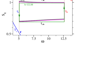
Figure 1: Three cycles of the heat engine in the ($\omega,{\cal S}_{E}$) plane. The common values are :$~{}J=2.,~{}T_{h}=7.5,~{}T_{c}=1.5,~{}~{}\omega_{a}=5.08364,~{}\omega_{b}=12.6355,~{}\Gamma_{h}=~{}\Gamma_{c}=1.16748,~{}\gamma_{h}=-0.05,~{}\gamma_{c}=-0.06$. $\Lambda_{ba}=\Lambda_{ab}=0$ for the black cycle,  $\Lambda_{ba}=~{}1.28,~{}\Lambda_{ab}=~{}0.64$ for the red cycle , and   $\Lambda_{ba}=122.88,~{}\Lambda_{ab}=61.44.$ for the green cycle. The time allocations on the different branches correspond to the optimal power point, when $\Lambda_{ba}=\Lambda_{ab}=0$. The optimal time allocations are: $\tau_{h}=1.0795~{}\tau_{ba}=0.01478,~{}\tau_{c}=1.0088~{},~{}\tau_{ab}=0.0069$. The points $\bf E$ and $\bf F$ represent the equilibrium points of the hot and cold isochores.

The cycle of the engine becomes a sequence of four completely positive maps that define the different branches. Eventually this sequence closes upon itself. Repetition of the sequence of controls leads to steady state operational conditions or a limit cycle Tova Feldmann and Ronnie Kosloff (2004). The map ${\cal U}_{k}$ relates the initial set of these operators to their final values for each of the engine branches. These maps are obtained by solving the equations of motion for the set of operators $\{{\bm{\mathrm{\hat{B}}}}\}$. The overall cycle map is the product of the individual maps of each branch ${\cal U}~{}~{}=~{}~{}{\cal U}_{ba}{\cal U}_{c}{\cal U}_{ab}{\cal U}_{h}$ Tova Feldmann and Ronnie Kosloff (2003, 2004).

On the isochores the maps ${\cal U}_{h/c}$ are generated by the completely positive generator ${\cal L}_{D}^{*}$ Lindblad (1976). Forcing detailed balance ${\cal L}_{D}^{*}$ leads to thermal equilibrium with a rate determined by $\Gamma$. In addition ${\cal L}_{D}^{*}$ also degrades the off diagonal elements of ${\bm{\mathrm{\hat{\rho}}}}_{e}$, interpreted either as decoherence or as dephasing. The dephasing time $T_{2}$ becomes identical to the energy equilibration time $T_{2}=T_{1}$. The dissipation has to also eliminate the additional energy accumulated on the adiabat. Degrading the coherences causes the frictional process to become irreversible Tova Feldmann and Ronnie Kosloff (2003, 2004). The interaction of the working medium with the bath can also be elastic. These encounters will scramble the phases conjugate to the energy, and the associated decay time is termed pure dephasing ($T_{2}^{*}$). In Lindblad’s formulation it becomes ${\cal L}^{\ast}_{D^{e}}({\bm{\mathrm{\hat{B}}}})=-\gamma[{\bm{\mathrm{\hat{H}}}},[{\bm{\mathrm{\hat{H}}}},{\bm{\mathrm{\hat{B}}}}]]$ and $T_{2}^{*}=1/2\gamma\Omega^{2}$. Note that elastic medium can not transfer or absorb heat, therefore we always need an inelastic medium.

On the adiabats, the varying field $\omega(t)$ causes an explicit time dependence of ${\bm{\mathrm{\hat{H}}}}$ $\frac{d{{\bm{\mathrm{\hat{B}}}}}}{dt}~{}~{}=~{}~{}i[{{\bm{\mathrm{\hat{H}}}}(t)},{{\bm{\mathrm{\hat{B}}}}}]$. Since the energy eigenvalues change, even if initially $[{{\bm{\mathrm{\hat{\rho}}}}},{{\bm{\mathrm{\hat{H}}}}}]=0$ the state ${\bm{\mathrm{\hat{\rho}}}}$ will develop off-diagonal terms in the energy frame (Cf. Eq. (B6) in Ref. Tova Feldmann and Ronnie Kosloff (2004)). The external power ${\cal P}=\dot{\omega}b_{1}$ can also be decomposed to the diagonal and off-diagonal terms in the energy representation:

$${\cal P}=\dot{\Omega}\frac{\langle{{\bm{\mathrm{\hat{H}}}}}\rangle}{\Omega}+\frac{{\dot{\omega}}J}{\Omega^{2}}\langle\left(J{{\bm{\mathrm{\hat{B}}}}_{1}}-\omega{{\bm{\mathrm{\hat{B}}}}_{2}}\right)\rangle~{}~{}~{}.$$ (11)

The first diagonal term represents the power required to compress or decompress the working fluid:

$${\cal P}_{ad}^{field}~{}~{}=~{}~{}\dot{\Omega}\frac{\langle{{\bm{\mathrm{\hat{H}}}}}\rangle}{\Omega}~{}~{},$$ (12)

the second term in Eq. (11) is the additional power required to drive the working fluid in a finite rate:

$${\cal P}_{ad}^{friction}~{}~{}=~{}~{}\frac{{\dot{\omega}}J}{\Omega^{2}}\langle\left(J{{\bm{\mathrm{\hat{B}}}}_{1}}-\omega{{\bm{\mathrm{\hat{B}}}}_{2}}\right)\rangle~{}~{}.$$ (13)

This term represents the power invested against friction therefore it vanishes when $J=0$ or $\dot{\omega}=0$ Tova Feldmann and Ronnie Kosloff (2000).

III Quantum Lubrication

A good lubricant should be able to increase the overall optimal power of the engine. The insight that energy coherences leads to frictional losses, suggests that forcing the cycle trajectory to follow adiabatically the instantaneous energy levels will be beneficial. A possible approach is to increase the dephasing on the isochores so that at the beginning of the adiabat $[{\bm{\mathrm{\hat{\rho}}}},{\bm{\mathrm{\hat{H}}}}]=0$. A thermal bath with strong dephasing will cause such an effect. We have found that an addition of pure dephasing has only a minor effect on the performance of the engine.

The quantum ”lubricant” has to suppress the creation of the energy coherences on the adiabats. Formally this can be described by a generator of dephasing in the equations of motion for the set $\{{{\bm{\mathrm{\hat{B}}}}}\}$ on the adiabat:

$$\frac{d{{\bm{\mathrm{\hat{B}}}}}}{dt}~{}~{}=~{}~{}i[{{\bm{\mathrm{\hat{H}}}}},{{\bm{\mathrm{\hat{B}}}}}]~{}~{}-~{}\Lambda[{\bm{\mathrm{\hat{H}}}},[\bf\hat{H},{\bm{\mathrm{\hat{B}}}}]]$$ (14)

and $\Lambda$ is the dephasing coefficient.

The success of this approach is shown in Fig. 2. As a reference the optimal power of the engine as a function of cycle time is shown around the global maximum. Each point on the graph is optimized with respect to the time allocations on the four branches of the cycle. Employing these time allocations the power of the engine is recalculated with the addition of the dephasing term on the adiabats. It is clear in Fig. 2 that in the interval of cycle times around the maximum power the ”lubricated” engine outperforms the optimal solutions of the reference engine. The ”lubricated” maximum power point also moves to shorter cycle times.

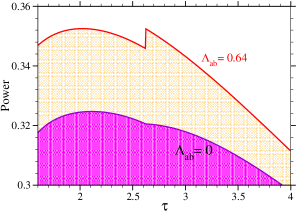
Figure 2: The optimal power as function of cycle time $\tau$ with and without the quantum ”lubricant”. The optimal time allocations are obtained for $\Lambda_{ba}=\Lambda_{ab}=0$ (blue line). The red line is the power with $\Lambda_{ba}=~{}1.28\Lambda_{ab}=~{}0.64$.  All the other parameters are as in Fig. 1.

For longer time allocations on the adiabats where less external power is consumed to overcome the friction, the performance enhancement due to dephasing decreased eventually leading to a crossover where dephasing on the adiabats decreased the power. For larger $J$ values we also found that dephasing was not able to improve the performance.

Fig. 3 shows the accumulated work against friction ${\cal W}^{friction}=\int{\cal P}^{friction}dt=\int\frac{\dot{\omega}J(b_{1}J-\omega b_{2})}{\Omega^{2}}dt$ (Cf. Eq. (13) ) as a function of time on the adiabat for increasing dephasing parameter. The main point is that increasing dephasing eliminates the work against friction. This improvement saturates once ${\cal W}^{friction}$ is eliminated.

Another consequence of the quantum lubrication is that the energy entropy ${\cal S}_{E}$ does not increase on the adiabats as can be seen in Fig. 1. As a result the energy entropy ${\cal S}_{E}$ approaches the von Neumann entropy ${\cal S}$, Eq. (9). These results establish the principle of quantum lubrication maintaining the working fluid in a diagonal state in the energy representation.

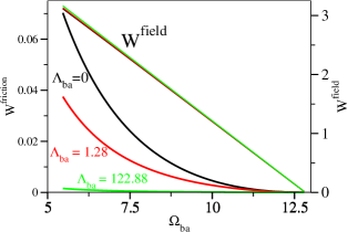
Figure 3: The work performed by the engine on the adiabat $b\rightarrow a$ branch, separated into $W^{friction}$ (left scale) and $W^{field}$ (right scale) for different dephasing values as a function of $\Omega_{ba}(t)$. $W^{field}$ has only a weak dependence on the dephasing value. The cycle parameter values are as in Fig. 1.

III.1 Dephasing synthesis

Suppression of friction requires a method to synthesize dephasing on the adiabats. The dynamics of the working medium has to be changed from unitary to dissipative. The obvious approach of adding a dissipative bath on the adiabatic branches is difficult to achieve. Such a bath should have only elastic encounters with a system with a time dependent Hamiltonian.

The solution is to employ the external controls of the engine to synthesize the dissipation. The idea comes from the singular bath limit, a bath generated from a system operator coupled to a delta correlated noise ${{\bm{\mathrm{\hat{H}}}}}_{sr}={{\bm{\mathrm{\hat{A}}}}_{s}}g(t)$ where $\langle g(t)g(t^{\prime})\rangle_{r}=\gamma\delta(t-t^{\prime})$ where the average is taken over the bath fluctuations. The Liouville generator associated with this system bath coupling becomes: ${\cal L}^{*}({{\bm{\mathrm{\hat{X}}}}})~{}~{}=~{}~{}-\frac{\gamma^{2}}{2}[{{\bm{\mathrm{\hat{A}}}}_{s}},[{{\bm{\mathrm{\hat{A}}}}_{s}},{{\bm{\mathrm{\hat{X}}}}}]]$ Gorini and Kossakowski (1976); R.S.Ingarden and Kossakowski (1975).

To implement such a scheme random noise is added to the external controls of the engine. The implementation divides the adiabat branch into $N$ segments. In each of these segments, the external field $\omega$ is constant and is chosen to be (for the $a\rightarrow b~{}$ adiabat): $\omega_{k}=\omega_{a}+\frac{\omega_{b}-\omega_{a}}{N}k$ for the $k$th segment. The short time propagator on the $k$ segment for the set ${\bm{\mathrm{\hat{B}}}}$ becomes:

$${\cal U}_{k}{{\bm{\mathrm{\hat{B}}}}}~{}~{}=~{}~{}e^{i{{\bm{\mathrm{\hat{H}}}}}(\omega_{k})\Delta t_{k}}~{}{{\bm{\mathrm{\hat{B}}}}}~{}e^{-i{{\bm{\mathrm{\hat{H}}}}}(\omega_{k})\Delta t_{k}}~{}~{},$$ (15)

where $\Delta t_{k}$ is the time interval of the $k$th segment. At this point random noise is added to the time interval

$$\Delta t_{k}~{}~{}=~{}~{}\frac{\tau_{ab}}{N}(1+r)$$ (16)

where $r$ is a random number with zero mean and variance $\sigma$. Expanding the propagator Eq. (15) to second order and averaging over the random noise will lead to the average generator for the $k$ time segment: ${\cal L}_{k}^{*}({{\bm{\mathrm{\hat{B}}}}})=i[{{\bm{\mathrm{\hat{H}}}}}(\omega_{k}),{{\bm{\mathrm{\hat{B}}}}}]-\frac{N\sigma^{2}}{2\tau_{ad}}[{{\bm{\mathrm{\hat{H}}}}}(\omega_{k}),[{{\bm{\mathrm{\hat{H}}}}}(\omega_{k}),{{\bm{\mathrm{\hat{B}}}}}]]$. In the limit when $N\rightarrow\infty$ this average propagator becomes identical to Eq. (14) provided $\sigma=\sqrt{\frac{2\tau_{ad}\Lambda}{N}}$.

The addition of random noise means that the individual cycle has to be replaced by the average performance on many cycles. As a result only an average cycle time can be defined. This noisy lubrication procedure was simulated with $N=200$ on both adiabats. The power and other thermodynamic variables were calculated as an average of 2000 cycles. Convergence was checked by continuing this averaging 1000 additional times.

Fig. 4 compares the Power ${\cal P}$ and entropy production per cycle, $\Delta S^{u}/\tau$ calculated by the two methods for the time allocations of the maximum power point. It is clear that the results obtained by imposing dephasing on the adiabats Eq. (14) are identical to the dephasing synthesis Eq. (15). The signature of lubrication is the reduction of entropy production which accompanies the increase in power. This is contrary to optimizing the power with respect to heat transport. In that case the increase in output power is accompanied by an increase in entropy production Tova Feldmann and Ronnie Kosloff (2000).

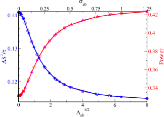
Figure 4: Power (right scale) and entropy production (left scale) as a function of the dephasing parameter $\Lambda_{ab}^{1/2}$ and the variance, $\sigma_{ab}$ of the random fluctuations of the time segment on the adiabats (upper scale). The dephasing synthesis results are represented by stars and filled triangles. The empty circles and squares represent the dephasing dynamics. The calculations were performed with $\frac{\Lambda_{ab}}{\Lambda_{ba}}=\frac{\sigma_{ab}}{\sigma_{ba}}$.

The choice of the procedure to generate dephasing is unique. For example, adding the random noise to the frequency $\omega_{k}$ at each time segment has been tested. The performance of the engine only became worse. The reason is that such a term leads to the dissipative generator ${\cal L}_{D}({{\bm{\mathrm{\hat{A}}}}})=-\frac{\gamma}{2}[{\bm{\mathrm{\hat{B}}}}_{1},[{\bm{\mathrm{\hat{B}}}}_{1},{\bm{\mathrm{\hat{A}}}}]]$ which does not eliminate the off diagonal elements in the energy representation.

The present study should be related to other recent works. For example, adding mechanical noise to a quantum refrigerator has been shown experimentally to cool atoms in a magnetic trap M. Kumakura, Y. Shirahata, Y. Takasu, Y. Takahashi and T. Yabuzaki (2003). It seems that the mechanism involves inducing non unitary dynamics. Contrary to the present study, in other scenarios coherence can be beneficial. Without violating the second law Scully et. al. M. O. Scully, M. S. Zubairy, G. S. Agarwal, H. Walther (2003) showed that additional work can be extracted from the coherences in quantum heat engine.

To summarize, frictional losses are caused whenever $[{\bm{\mathrm{\hat{H}}}}_{ext},{\bm{\mathrm{\hat{H}}}}_{int}]\neq 0$. Then the fast dynamics induces coherences in the energy frame. The essence of quantum lubrication is suppressing the generation of these off diagonal elements in the energy representation. The present model demonstrates how externally induced noise can achieve this task.