Robust “trapping states” in the motion of a trapped ion

Abstract

A novel robust mechanism for the generation of “trapping states” is shown to exist in the coupling of a two-level system with an oscillator, which is based on nonlinearities in the laser-induced vibronic coupling. This mechanism is exemplified with an ion confined in the potential well of a trap, where the nonlinearities are due to Franck–Condon type overlap integrals of the laser waves with the ionic centre-of-mass wavefunction. In contrast to the coherent trapping mechanism known from micro-maser theory, this mechanism works also in an incoherent regime operated by noisy lasers and is therefore much more robust against external decoherence effects. These features favour the incoherent regime, in particular for the preparation of highly excited trapping states.

, and

1 Introduction

Micro-maser theory predicts a coherent regime where so-called trapping states are created in the microwave cavity field, by injection of electronically prepared Rydberg atoms with well-defined velocities [1]. They are stable quantum states of the cavity field being unchanged by further interactions with injected atoms. The trapping states are photon-number states that represent a discrete, fixed number of cavity photons [2]. The preparation of trapping states with a pre-described photon number is performed by adjusting the atom-field interaction time, i.e., the velocity of the injected Rydberg atoms, to certain values. This mechanism crucially depends on a narrow velocity distribution of the atoms and is also very sensitive to any decoherence effects, such as cavity decay and thermalization via background radiation, or thermal motion of the cavity mirrors. Another limitation is the occurrence of (rare) two-atom events, that destroy the trapping states. This sensitivity is due to the fact, that the trapping mechanism relies on the coherent features of the Jaynes–Cummings dynamics [3]. Therefore, initially not a perfect photon-number state but sub-Poissonian photon statistics have been realised [4]. Later on, signatures of trapping states with small photon number could be successfully demonstrated [5]. When preparing trapping states of relatively large photon numbers, however, the above mentioned detrimental influence of decoherence poses an essential problem for the application of the coherent trapping mechanism.

Alternatively, a coherent Jaynes–Cummings type trapping mechanism can also be realized in the motion of a single trapped ion [6, 7, 8, 9]. Here the harmonic vibration of the trapped ion plays the role of the micro-maser cavity field, and the interaction of the injected Rydberg atoms with the micro-maser field is implemented by a combination of optical pumping and optical excitation of a vibrational sideband. As in the case of the micro-maser, this trapping mechanism for the vibration of a trapped ion also depends crucially on a coherent Jaynes–Cummings dynamics [7]. For a realistic experimental situation with phase-fluctuating laser fields obviously the coherent trapping mechanism is disturbed. In that case it has been shown that a sub-Poissonian, binomial statistics emerges for the vibrational quantum number of the trapped ion, that reveals a noise level being half of the classical shot noise [9].

The crucial point for realizing Jaynes–Cummings type trapping states in the motion of a trapped ion seems to be the need of a coherent time evolution without any decoherence effects. If one could use incoherent dynamics to prepare the desired states, all the above-mentioned problems could be avoided. Thus the question arises how to realize an incoherent dynamics that also gives rise to appropriate trapping-state conditions.

In this paper we propose a novel mechanism for the generation of “trapping states” in the vibration of a trapped ion that is based on nonlinearities occurring in the laser-induced vibronic interaction [10]. Dephasing effects emerging for example from phase-fluctuating laser fields or spontaneous emissions do not disturb this mechanism. Therefore, this incoherent regime is realistic and is also experimentally more feasible than the coherent dynamics needed for micro-maser-type trapping states. Moreover, the incoherent trapping mechanism may be less sensitive to other types of externally induced decoherence.

In Sec. 2 the laser-excitation scheme and the corresponding interaction Hamiltonians are discussed. In Sec. 3 we briefly summarise the realization of a coherent micro-maser-type dynamics, and in Sec. 4 the incoherent regime is introduced. A trapping mechanism that works also in the incoherent regime is then discussed in Sec. 5. Finally, a summary and some conclusions are given in Sec. 6.

2 Laser excitation scheme for the trapped ion

The centre-of-mass coordinate of a single ion bound in a radio-frequency trap, such as for example a Paul trap, is subject to a dynamics that can be described to good approximation as a 3D harmonic oscillation with three characteristic vibrational frequencies along the principal axes of the trapping potential. The geometry of the propagation of externally applied laser fields can be configured in such a way as to influence only the ion’s centre-of-mass motion in the direction of one principal axis, that is associated with the trap frequency $\nu$. Thus, one may consider the system as being one-dimensional, due to the natural decoupling from the remaining two other degrees of freedom [11].

In what follows, we always consider the case of quasi-monochromatic, collimated laser beams, whose wave-vectors are parallel to the chosen principal axis of the trap, that we may specify by the centre-of-mass coordinate $x$. In the case where laser-atom interactions are implemented by two-photon induced Raman transitions, the wave-vector of the beat note of the required two laser beams shall point along this axis.

The laser-excitation scheme shall consist of cycles, each being implemented by two interactions, an optical-pumping interaction, and a sideband interaction. The optical pumping is intended to invert the populations of the two states $|1\rangle$ and $|2\rangle$, cf. Fig. 1a.

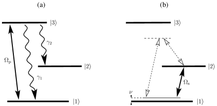
Figure 1: Laser-excitation scheme for the preparation of trapping state. During the optical-pumping interaction (a) a laser (Rabi frequency $\Omega_{\rm p}$) together with spontaneous emissions (rates $\gamma_{1,2}$) prepares the system in state $|2\rangle$. In the sideband interaction (b) the first vibrational sideband (vibration frequency $\nu$) is driven (Rabi frequency $\Omega_{\rm s}$) either directly (solid arrow) or in a Raman configuration (dashed arrows).

It is implemented via the laser-driven electric-dipole transition $|1\rangle\!\leftrightarrow\!|3\rangle$, and the spontaneous decay on the electric-dipole transition $|3\rangle\!\rightarrow\!|2\rangle$. The equation of motion, governing the dynamics of the vibronic density operator of the ion, $\hat{\varrho}$, is then given by

$$\dot{\hat{\varrho}} = -\frac{i}{\hbar}[\hat{H}_{0}\!+\!\hat{H}_{\rm p}(t),\hat{\varrho}]+\gamma_{1}\left(\hat{A}_{13}\,\hat{\mathcal{R}}_{1}[\hat{\varrho}]\,\hat{A}_{31}-{\textstyle\frac{1}{2}}\hat{A}_{33}\,\hat{\varrho}-{\textstyle\frac{1}{2}}\hat{\varrho}\,\hat{A}_{33}\right)$$ (1)

$$+\,\gamma_{2}\left(\hat{A}_{23}\,\hat{\mathcal{R}}_{2}[\hat{\varrho}]\,\hat{A}_{32}-{\textstyle\frac{1}{2}}\hat{A}_{33}\,\hat{\varrho}-{\textstyle\frac{1}{2}}\hat{\varrho}\,\hat{A}_{33}\right).$$

The operators $\hat{A}_{ij}\!=\!|i\rangle\langle j|$ induce transitions between the ion’s electronic states $|j\rangle$ and $|i\rangle$ and $\gamma_{1}$ and $\gamma_{2}$ are the spontaneous decay rates of state $|3\rangle$ decaying to states $|1\rangle$ and $|2\rangle$, respectively. The free Hamiltonian $\hat{H}_{0}$ reads

$$\hat{H}_{0}=\hbar\nu\,\hat{a}^{\dagger}\hat{a}+\sum_{i=1}^{3}\hbar\omega_{i}\hat{A}_{ii},$$ (2)

where $\hat{a}$ and $\hat{a}^{\dagger}$ are the annihilation and creation operators of vibrational quanta, respectively.

The laser interaction driving the optical pump process reads

$$\hat{H}_{\rm p}(t)={\textstyle\frac{1}{2}}\,\hbar\Omega_{\rm p}\,\hat{A}_{31}\,e^{-i\omega_{\rm p}t}+{\rm H.a.},$$ (3)

where $\Omega_{\rm p}$ is the Rabi frequency denoting the coupling strength of the pump laser beam with the electric-dipole moment of the ion. The pump-laser frequency $\omega_{\rm p}$ shall be near resonant with the electronic transition frequency $\omega_{31}$ of the states $|1\rangle$ and $|3\rangle$. For this interaction the laser beam is supposed to propagate along a direction perpendicular to the motional direction $x$ under consideration, to avoid coupling of the electronic and vibrational degrees of freedom in $x$ direction.

The photonic recoil acting on the centre-of-mass motion of the ion during the spontaneous emissions is given by the operator $\hat{\mathcal{R}}_{i}$ ($i\!=\!1,2$)

$$\hat{\mathcal{R}}_{i}[\hat{\varrho}]=\int_{-1}^{1}ds\,w(s)\,e^{is\eta_{i}(\hat{a}^{\dagger}+\hat{a})}\,\hat{\varrho}\,e^{-is\eta_{i}(\hat{a}^{\dagger}+\hat{a})},$$ (4)

with $w(s)\!=\!\frac{3}{8}(1\!+\!s^{2})$ describing the dipole radiation characteristics and the Lamb–Dicke parameters $\eta_{1}$ and $\eta_{2}$ correspond to the spontaneous transitions $|3\rangle\!\to\!|1\rangle$ and $|3\rangle\!\to\!|2\rangle$, respectively. For simplicity we neglect, for the moment, the vibrational scattering during the spontaneous photon emissions, i.e. we choose $\hat{\mathcal{R}}_{i}[\hat{\varrho}]\!\to\!\hat{\varrho}$, though later these effects will be taken into account to full extent numerically.

The stationary solution of the optical pumping process is approximately reached after a sufficiently long time of laser interaction. In terms of electronic-state matrix elements $\hat{\rho}_{ij}\!=\!\langle i|\hat{\varrho}|j\rangle$ of the density operator, that are still operators acting on the vibrational degree of freedom, the stationary solution reads

$$\hat{\rho}_{12}(\tau_{\rm p}) = \hat{\rho}_{23}(\tau_{\rm p})=\hat{\rho}_{31}(\tau_{\rm p})\approx 0$$ (5)

$$\hat{\rho}_{11}(\tau_{\rm p}) = \hat{\rho}_{33}(\tau_{\rm p})\approx 0$$ (6)

$$\hat{\rho}_{22}(\tau_{\rm p}) = \hat{U}_{0}(\tau_{\rm p})\left[\hat{\rho}_{11}(0)+\hat{\rho}_{22}(0)\right]\hat{U}_{0}^{\dagger}(\tau_{\rm p}).$$ (7)

Here we assume that initially, due to relaxation, the population in state $|3\rangle$ is zero, i.e., $\hat{\rho}_{33}(0)\!=\!0$. Thus, all population from state $|1\rangle$ merges with the population of state $|2\rangle$, while the ion is subject to oscillation in the trap potential.

The subsequent sideband interaction is implemented either by direct or by Raman excitation, resonant to the red vibrational sideband of the weak transition $|1\rangle\!\leftrightarrow\!|2\rangle$, cf. Fig. 1b. Its interaction Hamiltonian reads

$$\hat{H}_{\rm s}(t)={\textstyle\frac{1}{2}}\hbar\Omega\,\hat{A}_{21}\,e^{i(k\hat{x}-\omega t)}+{\rm H.a.},$$ (8)

where $k$ and $\omega$ are the projection of the wave-vector on the $x$ axis and the frequency, respectively, either of the laser field for direct excitation, or of the beat note of the Raman lasers. Moreover, the Rabi frequency $\Omega$ denotes the coupling strength of this transition. For the case of resonance with the red vibrational sideband, $\omega\!=\!\omega_{21}\!-\!\nu$, this laser interaction induces resonant vibronic transitions between states $|2\rangle|n\rangle$ and $|1\rangle|n\!+\!1\rangle$, where $|n\rangle$ are energy eigenstates of the centre-of-mass vibration in the trap potential. For this case the Hamiltonian (8) simplifies, in rotating-wave approximation and in the interaction picture, to a nonlinear Jaynes–Cummings type Hamiltonian [10],

$$\hat{H}_{\rm s}=\frac{1}{2}\hbar\Omega_{\rm s}\hat{A}_{21}\hat{f}(\hat{n};\eta)\,\hat{a}+{\rm H.a.}\;,$$ (9)

where $\Omega_{\rm s}\!=\!i\eta\Omega$ is the Rabi frequency on the red vibrational sideband in the Lamb–Dicke limit. The effects that arise in the regime beyond the Lamb–Dicke approximation, i.e., with rather large Lamb–Dicke parameter $\eta$ are described by the excitation-dependent operator function $\hat{f}(\hat{n};\eta)$ with $\hat{n}$ being the number operator of vibrational quanta in $x$ direction. Note, that for a Raman configuration, changing the laser-beam propagation geometry varies the projection $k$ of the beat-note wave-vector on the $x$ axis. Thus, the Lamb–Dicke parameter can be tuned up to rather large values.

The operator function $\hat{f}(\hat{n};\eta)$ depends solely on the number of vibrational quanta and can be given by a normally ordered expression as

$$\hat{f}(\hat{n};\eta) = e^{-\eta^{2}/2}\sum_{n=0}^{\infty}(-1)^{n}\frac{\eta^{2n}}{n!\,(n+1)!}\,\hat{a}^{\dagger n}\hat{a}^{n}$$

$$= :\,\left(\eta\sqrt{\hat{a}^{\dagger}\hat{a}}\right)^{-1}J_{1}\left(2\eta\sqrt{\hat{a}^{\dagger}\hat{a}}\right)\,:\,e^{-\eta^{2}/2},$$

where $:\,\,:$ denotes normal ordering, and $J_{k}(z)$ are the Bessel functions of integer order. Clearly these functions introduce a dependence of the laser-ion coupling on the vibrational excitation of the ion. They can be understood as analogy to Franck–Condon overlap integrals, however, in momentum space due to the recoil of absorbed and emitted photons.

For this approximation, i.e. neglecting spontaneous recoil effects, in each cycle of optical pumping and sideband interaction, the mean vibrational excitation will be increased or at least held constant. The dominant processes in one cycle can thus be given by the cascade

$$\begin{array}[]{l}|1\rangle|n\rangle\\ |2\rangle|n\rangle\end{array}\stackrel{{\scriptstyle\rm pump}}{{\Longrightarrow}}|2\rangle|n\rangle\stackrel{{\scriptstyle\rm sideband}}{{\Longrightarrow}}\begin{array}[]{l}|2\rangle|n\rangle\\ |1\rangle|n\!+\!1\rangle\end{array},$$

thus vibrational transitions $|n\rangle\!\rightarrow\!|n\rangle$ and $|n\rangle\!\rightarrow\!|n\!+\!1\rangle$ are performed in each cycle, leading to a net increase of the vibrational excitation.

3 Coherent time evolution

In the absence of decoherence effects the time evolution for the sideband interaction is described by a unitary time-evolution operator $\hat{U}(t)$. Thus, starting with the vibronic density operator $\hat{\varrho}$ of the trapped ion [cf. Eq. (7)]

$$\hat{\varrho}(t\!+\!\tau_{p})=\hat{A}_{22}\,\hat{U}_{0}(\tau_{p})\,\left[\hat{\varrho}_{11}(t)+\hat{\varrho}_{22}(t)\right]\,\hat{U}_{0}^{\dagger}(\tau_{p}),$$ (11)

at the time $t\!+\!\tau_{p}$, right after the optical pumping, the density operator reads after an interaction time $\tau_{s}$ of the sideband interaction,

$$\hat{\varrho}(t\!+\!\tau_{p}\!+\!\tau_{s})=\hat{U}_{\rm s}(\tau_{s})\,\hat{\varrho}(t\!+\!\tau_{p})\,\hat{U}_{\rm s}^{\dagger}(\tau_{s}),$$ (12)

where $\hat{U}_{\rm s}(t)\!=\!\hat{U}_{0}(t)\exp(-i\hat{H}_{\rm s}t/\hbar)$ and $\hat{U}_{0}(t)\!=\!\exp(-i\hat{H}_{0}t/\hbar)$.

Starting from an initial density operator at time $t_{k}$ we obtain the density operator at the time $t_{k+1}\!=\!t_{k}\!+\!\tau_{p}\!+\!\tau_{s}$, after a complete cycle of pump and sideband interaction, by insertion of Eq. (11) into (12) as

$$\hat{\varrho}(t_{k+1})=\hat{U}_{\rm s}(\tau_{s})\,|2\rangle\,\hat{U}_{0}(\tau_{p})\left[\langle 1|\hat{\varrho}(t_{k})|1\rangle\!+\!\langle 2|\hat{\varrho}(t_{k})|2\rangle\right]\hat{U}_{0}^{\dagger}(\tau_{p})\,\langle 2|\,\hat{U}_{\rm s}^{\dagger}(\tau_{s})$$ (13)

The vibrational number statistics is obtained from the density operator as

$$P_{n}(t)={\rm Tr}\left[\hat{\varrho}(t)\,|n\rangle\langle n|\right],$$ (14)

Using Eqs (13) and (14) straightforward calculation [13] results in a recurrence relation for the probabilities of vibrational quantum numbers

$$P_{n}(t_{k+1})=w_{\rm coh}(n|n\!-\!1)\,P_{n-1}(t_{k})+w_{\rm coh}(n|n)\,P_{n}(t_{k}),$$ (15)

where the probabilities for excitation or survival are characterised by a coherent sideband-interaction and read

$$w_{\rm coh}(n\!+\!1|n) = \sin^{2}\!\left[{\textstyle\frac{1}{2}}|\Omega_{\rm s}|\tau_{\rm s}\,f(n;\eta)\sqrt{n\!+\!1}\right],$$ (16)

$$w_{\rm coh}(n|n) = \cos^{2}\!\left[{\textstyle\frac{1}{2}}|\Omega_{\rm s}|\tau_{\rm s}\,f(n;\eta)\sqrt{n\!+\!1}\right],$$ (17)

where we have used the function $f(n;\eta)\!=\!\langle n|\hat{f}(\hat{n};\eta)|n\rangle$, which can be derived from Eq. (2) as Laguerre polynomial

$$f(n;\eta)=(n\!+\!1)^{-1}L_{n}^{(1)}(\eta^{2})\,e^{-\eta^{2}/2}.$$ (18)

Equation (15) describes the change of the vibrational statistics depending on the number of cycles performed. This recurrence relation contains the familiar trapping mechanism known from micro-maser theory [1]: The trapping state $|n_{0}\rangle$ is reached when the excitation rate (16) from state $|n_{0}\rangle$ to $|n_{0}\!+\!1\rangle$ vanishes, so that all the population accumulates in state $|n_{0}\rangle$. The condition $w_{\rm coh}(n_{0}\!+\!1|n_{0})\!=\!0$ thus leads to the condition for $|n_{0}\rangle$ being a trapping state:

$$|\Omega_{\rm s}|\tau_{\rm s}\,f(n_{0};\eta)\,\sqrt{n_{0}\!+\!1}=2\pi m,\quad m\in{\mathbb{Z}}.$$ (19)

In the Lamb–Dicke limit the nonlinear coupling function in Eq. (19) reduces to $\lim_{\eta\rightarrow 0}f(n;\eta)\!=\!1$, and Eq. (19) reduces to the familiar trapping-state condition for the micro-maser case [9]. This case is characterised by a non-vanishing function $f(n_{0};\eta)$, upon which the condition for the interaction time results

$$\tau_{\rm s}=\frac{2\pi m}{|\Omega_{\rm s}|f(n_{0};\eta)\sqrt{n_{0}\!+\!1}},\quad m\in{\mathbb{Z}}.$$ (20)

This type of trapping states is generated by a coherent mechanism, that consists of complete Rabi cycles at the trapping-state condition, leading to a locked vibrational quantum number.

Eq. (19) on the other hand, contains also a quite distinct type of trapping condition, namely that one where the Franck–Condon-type nonlinearity in the laser-ion coupling strength leads to a vanishing coupling, i.e., if

$$f(n_{0};\eta)=0.$$ (21)

This case does not correspond to complete Rabi cycles, but represents the breakdown of the laser-ion coupling mechanism, due to non-overlapping trap eigenstates in momentum representation, that are shifted off each other by the differing amount of the effective photonic momentum $\hbar k$. This novel type of trapping states may be set up in both a coherent or incoherent way.

Let us illustrate the qualitative differences between the two types of trapping states for a coherent sideband interaction and consider the two different ways of generating a trapping state $|n_{0}\rangle$ with $n_{0}\!=\!50$ vibrational quanta. The well known way is to use the standard trapping-state condition (20) to fix the pulse area $|\Omega_{\rm s}|\tau_{s}$ of the laser resonant with the vibrational sideband for a given Lamb–Dicke parameter $\eta$. The alternative way of generating this trapping state in a coherent fashion is given by adjusting the laser-beam geometry for sideband interaction (in a Raman configuration) in such a way as to tune to a Lamb–Dicke parameter that fulfils condition (21). The laser-pulse area is then chosen in such a way, that lower-lying trapping states due to complete Rabi cycles are avoided.

The improvement is illustrated when comparing the coherent transition rates $w_{\rm coh}(n\!+\!1|n)$ in the two cases, cf. Fig. 2.

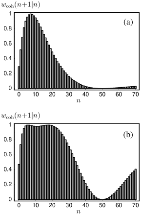
Figure 2: Coherent transition rates $w_{\rm coh}(n\!+\!1|n)$ for (a) $\eta\!=\!0.1$, $|\Omega_{\rm s}|\tau_{\rm s}\!=\!1.149$ [trapping-state condition (20) for $n_{0}\!=\!50$], and for (b) $\eta\!=\!0.268$ [trapping-state condition (21) for $n_{0}\!=\!50$] and $|\Omega_{\rm s}|\tau_{\rm s}\!=\!\pi/2$.

The dip of vanishing transition rate around the trapping state $|n_{0}\!=\!50\rangle$ is sharper for the rate shown in part (b), which is due to the nonlinear modification encoded in the function $f(n;\eta)$ when $\eta$ is not too small. As a consequence, when the quantum state approaches the trapping state $|n_{0}\!=\!50\rangle$, the dynamics is significantly slowed down in case (a) since the rates $w_{\rm coh}(n\!+\!1|n)$ are smaller (for $n\!=\!n_{0}\!-\!1,n_{0}\!-\!2,n_{0}\!-\!3$) as in case (b). In both cases the transition rates may be suppressed at certain vibrational numbers below the trapping state. These coherent effects emerge when the ion performs nearly complete Rabi cycles on the electronic transition at certain values of the integer $m$ in the trapping-state condition (20). Such subharmonic resonances degrade the generation of the trapping state, since they substantially decrease the flow of population into the trapping state.

The sensitivity to subharmonic resonances seems a handicap to both coherent ways of achieving a trapped state, in addition to the fundamental problem of preserving coherence. The novel scheme, however, evades both problems, since it is applicable in an incoherent way.

4 Incoherent dynamics

The trapping mechanisms described above, being based on coherent temporal evolution, are disturbed by any decoherence, as for example the phase fluctuations of the Raman lasers, or spontaneous emissions. It would be favourable to have a trapping mechanism at hand, that does not depend on the coherence of the underlying physical processes and is therefore not disturbed by such effects. Then, a trapping state might be reached even under the influence of various decohering perturbations and would be more robust than the micro-maser-type trapping states.

We consider the sideband interaction under the influence of decoherence, i.e. electronic dephasing, such as produced by phase-fluctuating lasers, spontaneous emissions, or collisions with background vapour. The total amount of phase fluctuations will be described by a dephasing rate $\gamma$ that gradually destroys the coherence between electronic levels $|1\rangle$ and $|2\rangle$. For simplicity we do not consider electronic dephasing mechanisms that depend on the vibrational excitation. Such effects may appear due to laser fluctuations [14], spontaneous Raman processes [15, 16], or combinations of both [17]. Moreover, for the analytic treatment we neglect the spontaneous recoil effects. These however will be included in the complete numerical solution shown later.

The master equation for the sideband-coupling interaction, including the decoherent phase fluctuations reads in the interaction picture as

$$\dot{\hat{\varrho}}=-\frac{i}{\hbar}[\hat{H}_{\rm s},\hat{\varrho}]-\frac{\gamma}{2}\left(\hat{A}_{11}\,\hat{\varrho}\,\hat{A}_{22}+\hat{A}_{22}\,\hat{\varrho}\,\hat{A}_{11}\right),$$ (22)

where the second term accounts for the electronic dephasing [18, 19]. The equations of motion for the electronic populations are derived from Eq. (22) as

$$\dot{\hat{\varrho}}_{11} = -\frac{i}{2}\left(\Omega_{\rm s}^{\ast}\,\hat{b}^{\dagger}\,\hat{\varrho}_{21}-\Omega_{\rm s}\,\hat{\varrho}_{12}\,\hat{b}\right),$$ (23)

$$\dot{\hat{\varrho}}_{22} = -\frac{i}{2}\left(\Omega_{\rm s}\,\hat{b}\,\hat{\varrho}_{12}-\Omega_{\rm s}^{\ast}\,\hat{\varrho}_{21}\,\hat{b}^{\dagger}\right),$$ (24)

where we have made use of the nonlinearly deformed annihilation operator

$$\hat{b}=\hat{f}(\hat{a}^{\dagger}\hat{a};\eta)\,\hat{a}.$$ (25)

The time evolution of the electronic coherences, on the other hand, is modified

$$\dot{\hat{\varrho}}_{12} = -\frac{\gamma}{2}\,\hat{\varrho}_{12}-\frac{i}{2}\Omega_{\rm s}^{\ast}\left(\hat{b}^{\dagger}\hat{\varrho}_{22}-\hat{\varrho}_{11}\,\hat{b}^{\dagger}\right),$$ (26)

$$\dot{\hat{\varrho}}_{21} = -\frac{\gamma}{2}\,\hat{\varrho}_{21}-\frac{i}{2}\Omega_{\rm s}\left(\hat{b}\,\hat{\varrho}_{11}-\hat{\varrho}_{22}\,\hat{b}\right).$$ (27)

Let us now consider the incoherent regime where the dephasing rate $\gamma$ is larger than the Rabi frequency on the vibrational sideband: $\gamma\!>\!|\Omega_{\rm s}|$. Nevertheless, we consider the case of well-resolved sidebands, $\nu\!>\!\gamma$, and thus $\gamma$ is in the range given by

$$|\Omega_{\rm s}|<\gamma<\nu.$$ (28)

Then the rotating-wave approximation with respect to $\nu$ for the derivation of Eq. (9) is valid. For typical vibrational frequencies of $\nu/2\pi\!\approx\!1\!\ldots\!10$ MHz and Rabi frequencies of $|\Omega|/2\pi\!\approx\!10\!\ldots\!100$ kHz, the dephasing rate is supposed on the order of $\gamma/2\pi\!\approx\!100\mbox{ kHz}\ldots\!1\mbox{ MHz}$. In this incoherent regime adiabatic elimination of the electronic coherences can be performed by neglecting the time derivatives in Eqs. (26) and (27) and solving for the electronic coherences. Inserting the resulting electronic coherences into the equations of motion for the electronic populations (23) and (24) we obtain

$$\dot{\hat{\varrho}}_{11} = \frac{|\Omega_{\rm s}|^{2}}{\gamma}\left(\hat{b}^{\dagger}\hat{\varrho}_{22}\,\hat{b}-{\textstyle\frac{1}{2}}\hat{b}^{\dagger}\hat{b}\,\hat{\varrho}_{11}-{\textstyle\frac{1}{2}}\hat{\varrho}_{11}\,\hat{b}^{\dagger}\hat{b}\right),$$ (29)

$$\dot{\hat{\varrho}}_{22} = \frac{|\Omega_{\rm s}|^{2}}{\gamma}\left(\hat{b}\,\hat{\varrho}_{11}\,\hat{b}^{\dagger}-{\textstyle\frac{1}{2}}\hat{b}\hat{b}^{\dagger}\hat{\varrho}_{22}-{\textstyle\frac{1}{2}}\hat{\varrho}_{22}\,\hat{b}\hat{b}^{\dagger}\right).$$ (30)

These equations can be decoupled and solved by use of the dressed-state coefficients

$$C_{mn}^{(\pm)}=\langle m|\hat{\varrho}_{11}|n\rangle\pm\langle m\!-\!1|\hat{\varrho}_{22}|n\!-\!1\rangle.$$ (31)

From Eqs. (29) and (30) we obtain the decoupled differential equations for the coefficients $C_{mn}^{(\pm)}(t)$ as

$$\dot{C}_{mn}^{(\pm)}=-{\textstyle\frac{1}{4}}\left[\sqrt{\gamma_{m\!-\!1}(\eta)}\mp\sqrt{\gamma_{n\!-\!1}(\eta)}\right]^{2}C_{mn}^{(\pm)},$$ (32)

where the excitation-dependent damping coefficients are given by

$$\gamma_{n}(\eta)=2\gamma s\,(n\!+\!1)\,[f(n;\eta)]^{2},$$ (33)

and the saturation parameter reads $s\!=\!2|\Omega_{\rm s}|^{2}/\gamma^{2}$. Using Eq. (18) the nonlinear damping coefficients can be given in terms of Laguerre polynomials as

$$\gamma_{n}(\eta)=\frac{2\gamma s}{n\!+\!1}\,|L_{n}^{(1)}(\eta^{2})|^{2}\,e^{-\eta^{2}}.$$ (34)

Note, that the laser-ion coupling nonlinearity appears only in these damping coefficients, and that in the Lamb–Dicke approximation they become linear with $n$:

$$\lim_{\eta\rightarrow 0}\gamma_{n}(\eta)=2\gamma s\,(n\!+\!1).$$ (35)

The vibrational number statistics $P_{n}$ can be easily obtained from the matrix elements $C_{mn}^{(\pm)}$ as follows:

$$P_{n}={\textstyle\frac{1}{2}}\left(C_{nn}^{(+)}\!+\!C_{nn}^{(-)}\!+\!C_{n+1,n+1}^{(+)}\!-\!C_{n+1,n+1}^{(-)}\right).$$ (36)

Thus only the diagonal matrix elements $C_{nn}^{(\pm)}$ are needed, which obey the equations of motion

$$\dot{C}_{nn}^{(+)}=0,\quad\dot{C}_{nn}^{(-)}=-\gamma_{n\!-\!1}(\eta)\,C_{nn}^{(-)}.$$ (37)

Since the incoherent dynamics of the sideband interaction follows the optical pumping, the initial conditions for the density-matrix elements can be written as

$$\langle n|\hat{\varrho}_{11}(t_{k}\!+\!\tau_{\rm p})|n\rangle = 0,$$ (38)

$$\langle n|\hat{\varrho}_{22}(t_{k}\!+\!\tau_{\rm p})|n\rangle = P_{n}(t_{k}\!+\!\tau_{\rm p})=P_{n}(t_{k}),$$ (39)

where again $t_{k}$ denotes the time after a complete cycle, and $\tau_{p}$ is the pump time. Using these initial conditions one obtains, via Eq. (31), the initial conditions for the coefficients and the solution of Eq. (37) results as

$$C_{nn}^{(+)}(t_{k+1}) = P_{n-1}(t_{k}),$$ (40)

$$C_{nn}^{(-)}(t_{k+1}) = -P_{n-1}(t_{k})\,\exp[-\gamma_{n\!-\!1}(\eta)\,\tau_{\rm s}],$$ (41)

Inserting Eqs. (40) and (41) into Eq. (36) one finally obtains a modified recurrence relation for the number statistics after subsequent cycles in the incoherent regime

$$P_{n}(t_{k+1})=w_{\rm inc}(n|n\!-\!1)\,P_{n\!-\!1}(t_{k})+w_{\rm inc}(n|n)\,P_{n}(t_{k}),$$ (42)

with the transition rates in the incoherent regime of sideband interaction,

$$w_{\rm inc}(n\!+\!1|n) = {\textstyle\frac{1}{2}}\left\{1-\exp[-\gamma_{n}(\eta)\,\tau_{\rm s}]\right\},$$ (43)

$$w_{\rm inc}(n|n) = {\textstyle\frac{1}{2}}\left\{1+\exp[-\gamma_{n}(\eta)\,\tau_{\rm s}]\right\}.$$ (44)

5 Incoherent trapping mechanism

Let us now study in more detail the rates $w_{\rm inc}(n\!+\!1|n)$, that determine the increase of the mean vibrational excitation. If those rates are non-vanishing, the populations of vibrational quantum numbers will be shifted to the next higher lying quantum numbers in each cycle, leading to an overall increase of the mean vibrational excitation. If, however, $w_{\rm inc}(n_{0}\!+\!1|n_{0})$ is zero for some vibrational number $n_{0}$, the recurrence relation (42) has a cutoff at that number $n_{0}$. That is, all populations that were initially at vibrational quantum numbers below $n_{0}$ will be accumulated after some time in the vibrational state $|n_{0}\rangle$. Clearly, populations in levels higher than $n_{0}$ will be shifted to still higher quantum numbers in each cycle.

Thus two distinct dynamical regimes can be found in the incoherent dynamics: A regime where the mean vibrational excitation is increased in each cycle, and a trapping regime for populations initially below a certain vibrational quantum number $n_{0}$ where the condition $w_{\rm inc}(n_{0}\!+\!1|n_{0})\!=\!0$ holds. The latter we will call, in the following, incoherent trapping states since they emerge from a dynamics bare of any coherence.

In fact, incoherent trapping states emerge from a breakdown of the ion-laser coupling and are thus related to the second type of trapping states with coherent dynamics discussed before. To see this relation, let us consider the condition for an incoherent trapping state at vibrational quantum number $n_{0}$:

$$w_{\rm inc}(n_{0}\!+\!1|n_{0})=0={\textstyle\frac{1}{2}}\left\{1-\exp\left[-\gamma_{n_{0}}(\eta)\,\tau_{\rm s}\right]\right\},$$ (45)

which is equivalent to the condition

$$\gamma_{n_{0}}(\eta)=0.$$ (46)

From their definition (33) follows $\gamma_{n_{0}}(\eta)\!\propto\![f(n_{0};\eta)]^{2}$, such that the condition for incoherent trapping states (46) is equivalent to the condition of nonlinear coherent trapping states (21). This is because both types of trapping states rely on the same mechanism, namely, the breakdown of the laser-ion coupling strength due to the vanishing of Franck–Condon type overlap integrals of vibrational wave functions. Thus, we deal with a trapping mechanism that appears both in the coherent and the incoherent regime and therefore does not rely on coherent dynamics.

Incoherent trapping states may be conveniently prepared with no need for coherence. Decoherence effects will not prevent the emergence of these trapping states. For small vibrational quantum numbers one typically would need only few cycles such that little decoherence is accumulated. However, for generating highly excited vibrational number states, the mechanism of incoherent trapping states is superior. Then a rather large number of cycles is required, where in each cycle decoherence effects would eventually prevent any coherent mechanism from working.

Let us now study the dynamic increase of the vibrational excitation in the incoherent regime. For large saturation $s$ and/or large interaction times $\tau_{\rm s}$, the transition rates $w_{\rm inc}$ can be approximated as

$$w_{\rm inc}(n\!+\!1|n) \approx \frac{1}{2}\Big{[}1-\sum_{n_{0}(\eta)}\delta_{n,n_{0}(\eta)}\Big{]},$$ (47)

$$w_{\rm inc}(n|n) \approx \frac{1}{2}\Big{[}1+\sum_{n_{0}(\eta)}\delta_{n,n_{0}(\eta)}\Big{]},$$ (48)

where $\delta_{n,m}$ denotes the Kronecker delta symbol and the sum extends over all possible trapping numbers $n_{0}(\eta)$ at the given Lamb–Dicke parameter $\eta$. This form of the transition rates is an excellent approximation for a wide range of parameters and holds for the following examples. Thus, in regions of vibrational numbers $n\!\neq\!n_{0}(\eta)$, the transition rates simplify to

$$w_{\rm inc}(n\!+\!1|n)\approx w_{\rm inc}(n|n)\approx\frac{1}{2},$$ (49)

and the recurrence relation (42) for the incoherent dynamics reduces to

$$P_{n}(t_{k+1})={\textstyle\frac{1}{2}}\,P_{n}(t_{k})+{\textstyle\frac{1}{2}}\,P_{n-1}(t_{k}).$$ (50)

Due to the constant transition rates, now the evolution towards a trapping state is not slowed down by quasi-trapping conditions as may be found in the coherent rates.

Using Eq. (50) it can be shown that, far from any trapping state, the mean vibrational excitation and variance obey the following dynamics:

$$\langle\hat{n}(t_{k+1})\rangle = \langle\hat{n}(t_{k})\rangle+{\textstyle\frac{1}{2}},$$ (51)

$$\langle\left[\Delta\hat{n}(t_{k+1})\right]^{2}\rangle = \langle\left[\Delta\hat{n}(t_{k})\right]^{2}\rangle+{\textstyle\frac{1}{4}}.$$ (52)

These relations show that in each cycle, on the average, half a vibrational quantum is created in the ionic motion. Moreover, the mean excitation increases faster than the variance so that for a large number of cycles $k$ the relative variance $\langle\Delta\hat{n}^{2}\rangle/\langle\hat{n}\rangle$ reaches the stationary value,

$$\lim_{k\rightarrow\infty}\frac{\langle\left[\Delta\hat{n}(t_{k})\right]^{2}\rangle}{\langle\hat{n}(t_{k})\rangle}=\frac{1}{2}.$$ (53)

A statistics of this type corresponds to a noise level half the shot-noise limit and is a signature for amplitude squeezing. In fact, the solution of Eq. (50) can be given as a sum of Binomial distributions, each with vibrational mean number $l\!+\!k/2$ and variance $k/4$, that are weighted by the initial number statistics $P_{l}(t_{0})$:

$$P_{n}(t_{k})=\sum_{l=0}^{n}{k\choose n\!-\!l}\left(\frac{1}{2}\right)^{k}P_{l}(t_{0}).$$

Near the trapping state $|n_{0}\rangle$, however, the relative variance deviates from the stationary value (53), decreases below $1/2$ and reaches zero when the trapping state is finally populated with unit probability.

Clearly, this behaviour is idealised by the fact that spontaneous recoil effects during the periods of optical pumping have been neglected in the analysis. However, using quantum-trajectory methods we have included these effects consistently to obtain numerical results. These results, that will be shown in the following, are based on the parameters $\gamma_{1}/\nu\!=\!9.5$, $\gamma_{2}/\nu\!=\!3.3$, $\eta_{1}\!\approx\!\eta_{2}\!=\!0.142$, and $|\Omega_{\rm p}|^{2}/\gamma_{1}^{2}\!=\!5.0$ for the optical pumping processes.

In Fig. 3 the numerical results for the relative variance of vibrational quanta is shown in dependence on the number of cycles for the incoherent trapping state $|n_{0}\!=\!50\rangle$ for varying effective saturations $\gamma s\tau_{s}$. It can be observed that for the larger values of $\gamma s\tau_{s}$ the relative variance transiently tends to the value $0.5$, but then increases due to the photon scattering until the trapping state is approached. There the relative variance decreases even below $0.5$, but only as a local minimum, to monotonically increase afterwards. Furthermore, for low “saturation” (see dotted curve) the Binomial regime is not even reached as an initial transient behaviour.

Figure 3: Relative variance versus the number of cycles $k$ for the incoherent trapping state $|n_{0}\!=\!50\rangle$ with $\eta\!=\!0.268$. Spontaneous recoil effects during the optical pumping are included; saturation parameter is $\gamma s\tau_{\rm s}\!=\!0.2\mbox{ (dotted)},1.0\mbox{ (solid)},2.0\mbox{ (dashed)}$.

These results show that due to the recoil effects in the optical pumping the trapping states are not truly stationary. Instead the vibrational populations cross the trapping state to later be partly accumulated at approximately equidistant further trapping states at $n_{0}\!\approx\!100,150,200,\ldots$. However, it should be kept in mind that the relative variance is very sensitive to minimal populations at high vibrational quantum numbers. Thus a low percentage of population distributed around or higher than the trapping state drastically increases the relative variance. In this sense a more suitable property is the maximum population reached in the trapping state.

An example is shown in Fig. 4 where vibrational statistics is shown at different stages of the evolution for the same trapping state $|50\rangle$. In fact it can be seen that the higher the value of $\gamma s\tau_{s}$ the higher the population in the trapping state at cycle $k\!=\!200$. Clearly in the further time evolution this population decreases again by scattering events that eventually distribute the population at higher vibrational levels. Nevertheless, if the laser interactions are stopped appropriately when a high population in the trapping state is reached, maximum populations up to $60\%$ at the level $n_{0}\!=\!50$ can be obtained.

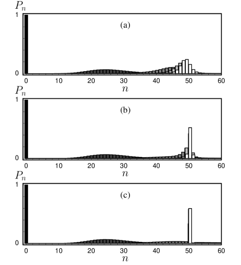
Figure 4: Incoherent dynamics, including spontaneous recoil effects, of vibrational populations for $k\!=\!0,50,100,150,200$ cycles (gray scales from black to white) and Lamb–Dicke parameter $\eta\!=\!0.268$ with trapping state $|n_{0}\!=\!50\rangle$. Other parameters are $\gamma s\tau_{s}\!=\!1\mbox{ (a)},10\mbox{ (b)},1000\mbox{ (c)}$.

It is noteworthy that for decreasing Lamb–Dicke parameters the trapping states have increasing energies. In Fig. 5 we show certain combinations of Lamb–Dicke parameters and vibrational quantum numbers $n_{0}$, that satisfy trapping. These are directly obtained from condition (46), together with Eq. (34).

Figure 5: Pairs of values for the trapping state number $n_{0}$ and the Lamb–Dicke parameter $\eta$ that obey the nonlinear trapping-state condition [Eq. (21)].

As to practical implementation of the incoherent method, experiments on a single ion have been performed that indicate breakdown of the ion-laser coupling at small values of the Lamb–Dicke parameter and rather highly excited trap levels [6, 20]. In these experiments certain metastable states of the ion’s vibrational amplitude with $5\mbox{--}30\mu{\rm m}$ spatial extension within the $400\mu{\rm m}$-wide focus of saturating laser light have been observed. In steady state, one of these metastable states was found occupied by the unperturbed, moderately laser-cooled ion. The ion jumped to another one upon external perturbation: small variation of the cooling power by minute laser detuning, irradiation by a weak pulse of resonant radio frequency ($1\mbox{--}2$MHz, typically), etc. Each stable amplitude corresponds to a number of mean vibrational excitation that is associated with a particular level, a trapping level, where the laser-ion coupling breaks down for the given small Lamb–Dicke parameter. Thus the nonlinearity in the laser-ion coupling as discussed here, is of great importance even with a small Lamb–Dicke parameter $\eta$ that makes trapping states appear at very large vibrational quantum numbers. These observations demonstrate that an individual ion confined in a harmonic potential well indeed may be prepared in a highly excited incoherent trapping state.

6 Summary and conclusions

We have studied ways of generating various kinds of “trapping states” of the quantised centre-of-mass motion of a trapped ion. The first kind is of the micro-maser type. In this case, the ion, at a particular vibrational quantum number, undergoes a complete Rabi cycle of excitation, such that higher quantum states cannot become excited. This mechanism, however, is highly fragile with respect to any kind of decoherence. Moreover, when one intends to prepare a certain vibrational number state, quasi-trapping conditions may exist for other (lower) number states. This feature leads to a substantial increase of the time needed for the preparation.

Another way of implementing a trapping-state condition is based on the nonlinearities that appear in the dependence of the atom-field coupling on the vibrational excitation. These nonlinearities arise as Franck–Condon-type overlap integrals due to the exchange of momentum between the ion’s centre-of-mass motion and the absorbed and emitted laser photons. At certain vibrational quantum numbers the nonlinearly modified interaction strength vanishes, leading to the expected trapping states in a way quite different from the trapping mechanism based on the completion of Rabi cycles. This trapping mechanism, when used in its coherent version, reduces the preparation time, although this method is still highly sensitive with respect to decoherence.

The particular advantage of the nonlinearity-based trapping condition consists in the vanishing coupling for certain vibrational excitations. This feature can be exploited for the generation of trapping states even in situations where substantial decoherence prevails, since now the trapping state is solely determined by the selected Lamb–Dicke parameter. Moreover, the transition rates for approaching the trapping state are more or less independent of the vibrational excitation, which leads to substantial decrease of the time needed to prepare a desired trapping state. Thus, one avoids the sensitivity to decoherence, especially when preparing vibrational number states of large quantum numbers.

References

- [1] P. Filipowicz, J. Javanainen, and P. Meystre, Phys. Rev. A 34 (1986) 3077.
- [2] It should be pointed out that also other concepts of “trapped states” exist, cf. H.-I. Yoo and J.H. Eberly, Phys. Rep. 118, 239 (1985).
- [3] E.T. Jaynes and F.W. Cummings, Proc. IEEE, vol. 51 (1963) p. 89.
- [4] G. Rempe, F. Schmidt–Kaler, and H. Walther, Phys. Rev. Lett. 64 (1990) 2783.
- [5] M. Weidinger, B.T.H. Varcoe, R. Heerlein, and H. Walther, Phys. Rev. Lett. 82 (1999) 3795.
- [6] Th. Sauter, H. Gilhaus, I. Siemers, R. Blatt, W. Neuhauser, and P.E. Toschek, Z. Phys. D 10 (1988) 153.
- [7] C.A. Blockley, D.F. Walls, and H. Risken, Europhys. Lett. 17 (1992) 509.
- [8] R. Blatt, J.I. Cirac, and P. Zoller, Phys. Rev. A 52 (1995) 518.
- [9] S. Wallentowitz, W. Vogel, I. Siemers, and P.E. Toschek, Phys. Rev. A 54 (1996) 943.
- [10] W. Vogel and R.L. de Matos Filho, Phys. Rev. A 52 (1995) 4214.
- [11] J. Eschner, B. Appasamy, and P.E. Toschek, Opt. Commun. 118 (1995) 123.
- [12] Note, that level in Fig. 1a, used for optical pumping, can be different from the level in Fig. 1b, used for Raman driving the transition , to allow for independent control of Lamb–Dicke parameters.
- [13] For a review on laser-induced nonlinear vibronic couplings of trapped ions, see W. Vogel and S. Wallentowitz, Manipulation of the quantum state of a trapped ion, in Coherence and statistics of photons and atoms, ed. J. Perina (Wiley, New York, 2001).
- [14] S. Schneider and G.J. Milburn, Phys. Rev. A 57, 3748 (1998).
- [15] C. Di Fidio, S. Wallentowitz, Z. Kis, and W. Vogel, Phys. Rev. A 60, R3393 (1999).
- [16] C. Di Fidio and W. Vogel, Phys. Rev. A 62, 031802(R) (2000).
- [17] A.A. Budini, R.L. de Matos Filho, and N. Zagury, Phys. Rev. A 65, 041402(R) (2002).
- [18] G.S. Agarwal, Phys. Rev. Lett. 37 (1976) 1383; 1773.
- [19] J.H. Eberly, Phys. Rev. Lett. 37 (1976) 1387.
- [20] Th. Sauter, H. Gilhaus, W. Neuhauser, R. Blatt, and P.E. Toschek, Europhys. Lett. 7 (1988) 317.