Physical Purification of Quantum States

Abstract

We introduce the concept of a physical process that purifies a mixed quantum state, taken from a set of states, and investigate the conditions under which such a purification map exists. Here, a purification of a mixed quantum state is a pure state in a higher-dimensional Hilbert space, the reduced density matrix of which is identical to the original state. We characterize all sets of mixed quantum states, for which perfect purification is possible. Surprisingly, some sets of two non-commuting states are among them. Furthermore, we investigate the possibility of performing an imperfect purification.

I Introduction

A fundamental entity in quantum mechanics and quantum information is a mixed quantum state. A mixed quantum state can be either understood as a statistical mixture of pure quantum states, or as being part of a higher-dimensional, pure state – a purification of the mixed state. Formally, given the decomposition $\rho=\sum_{i}p_{i}{{|{\chi_{i}}\rangle\!\langle{\chi_{i}}|}}$, where $p_{i}\geq 0$ and $\sum_{i}p_{i}=1$, an example for a purification of $\rho$ is given by ${|\psi\rangle}=\sum_{i}\sqrt{p_{i}}{|\chi_{i}\rangle}{|a_{i}\rangle}$, with the auxiliary states ${|a_{i}\rangle}$ being mutually orthogonal. This abstract point of view was, so far, the main impetus for discussing purifications of a single, known quantum state Hughston et al. (1993); Bassi and Ghirardi (2003).

In this paper, we consider the purification of an unknown quantum state. More precisely, we introduce the fundamental question whether there exists a physical process (i.e. a completely positive map) that takes any state of a given set to one of its purifications. (We remind the reader for clarity that there exists a different notion of “purification” in the literature, referring to the process of performing operations on several identical copies of a given state, such that the purity of some of them is increased; a typical application is entanglement distillation.) Our aim is to characterize all sets of states for which a purifying map exists. The existence of such a process implies a non-trivial physical equivalence between certain sets of mixed and pure quantum states.

Let us introduce our concepts and outline the structure of this paper. As already pointed out above, a purification of a mixed state has to satisfy two characteristic properties: first, it has to be pure, and second, tracing out the auxiliary system has to yield back the original state. We call the second property faithfulness and name a process a perfect purifier for a mixed state, when the output achieves both properties. It is straightforward to prove that the linearity of quantum mechanics does not allow the existence of a perfect purifier for a completely unknown quantum state, i.e. a state taken from the set of all states. However, will dropping the condition of faithfulness or the one of purity allow non-trivial purification processes for an unknown quantum state? It will be shown in Theorem 1 that this is not the case. Consequently, in Section III we will restrict the set of possible input states, and investigate the properties of purifying maps acting on the most simple non-trivial set, namely a set of only two mixed states. While keeping the condition of purity, we will find that the deviation from perfect faithfulness depends on a purely geometric quantity of the two inputs. This result will allow us to derive lower and upper bounds on the achievable faithfulness. Since these bounds do not exclude perfect faithfulness for certain pairs of states, we then in Section IV proceed to investigate the existence of a perfect purifier in general. Theorem 2 completely characterizes all sets of states that can be purified perfectly. Finally, we will provide an operational test for a given pair of states that allows to check whether a physical purification is possible.

II The general purification task

In the following we will denote by ${\mathcal{M}}$ a given set of mixed states, represented by density operators that act on a finite-dimensional Hilbert space ${\mathcal{H}}$. The elements $\rho_{i}\in{\mathcal{M}}$ are allowed to have unbalanced a priori probabilities $\eta_{i}>0$, satisfying $\sum_{i}\eta_{i}=1$. We consider deterministic physical processes represented by completely positive and trace preserving linear maps $\Lambda$ that take any density operator acting on ${\mathcal{H}}$ to a density operator acting on ${\mathcal{H}}\otimes{{\mathcal{H}}_{\mathrm{aux}}}$, where ${{\mathcal{H}}_{\mathrm{aux}}}$ denotes an auxiliary space of unspecified dimension. We refer to such a physical process as a perfect purifier if for each $\rho_{i}\in{\mathcal{M}}$, the output $\Lambda[\rho_{i}]$ is pure as well as faithful, i.e. ${\operatorname{tr}_{\mathrm{aux}}}\Lambda[\rho_{i}]=\rho_{i}$. If these conditions are not met, we will measure the average output purity by $\mathsf{p}=\sum_{i}\eta_{i}\operatorname{tr}\Lambda[\rho_{i}]^{2}$ and the average faithfulness by $\mathsf{f}=1-\sum_{i}\eta_{i}{\|{\rho_{i}-{\operatorname{tr}_{\mathrm{aux}}}\Lambda[\rho_{i}]}\|}$. Here, ${\|{\rho-\sigma}\|}=\frac{1}{2}\operatorname{tr}|\rho-\sigma|$ denotes the trace distance, where $|A|=\sqrt{A^{\dagger}A}$. The trace distance is a good measure for the distinguishability of two states as it vanishes for identical states and is equal to one for orthogonal states. In particular the success probability for the minimum error discrimination procedure Helstrom (1976); Herzog and Bergou (2004) of two states having equal a priori probability depends linearly on the trace distance of the states. – We call any deterministic process a purifier of ${\mathcal{M}}$, if it does not decrease the average purity of ${\mathcal{M}}$.

For the universal case where the set ${\mathcal{M}}$ contains all possible density operators acting on a given Hilbert space, neither relaxing the condition of purity nor relaxing the condition of faithfulness allows non-trivial purifiers:

Theorem 1.

(i) Any universal purifier with perfect output purity is a constant map. (ii) A universal purifier with perfect faithfulness does not increase the purity of any state.

Proof.

We prove (i) by contradiction. Suppose there exists a purifier $\Lambda$ such that $\Lambda[\rho]$ is pure for any state $\rho$, and with the property that at least for two states $\rho_{1}$ and $\rho_{2}$, $\Lambda[\rho_{1}]\neq\Lambda[\rho_{2}]$ holds. But for the state $\rho_{3}=(\rho_{1}+\rho_{2})/2$, the purity of $\Lambda[\rho_{3}]=(\Lambda[\rho_{1}]+\Lambda[\rho_{2}])/2$ requires $\Lambda[\rho_{1}]=\Lambda[\rho_{2}]$.

Proof of statement (ii): perfect faithfulness of a universal purifier requires that any pure state ${{|{\phi}\rangle\!\langle{\phi}|}}$ is mapped onto the state ${{|{\phi}\rangle\!\langle{\phi}|}}\otimes\sigma_{\phi}$ for some state $\sigma_{\phi}$ acting on ${{\mathcal{H}}_{\mathrm{aux}}}$. For any state $\rho$ we find with the spectral decomposition $\rho=\sum p_{i}{{|{\lambda_{i}}\rangle\!\langle{\lambda_{i}}|}}$ that due to linearity $\operatorname{tr}\Lambda[\rho]^{2}=\operatorname{tr}(\sum_{i}p_{i}{{|{\lambda_{i}}\rangle\!\langle{\lambda_{i}}|}}\otimes\sigma_{\lambda_{i}})^{2}=\sum_{i}p_{i}^{2}\operatorname{tr}\sigma_{\lambda_{i}}^{2}\leq\sum_{i}p_{i}^{2}=\operatorname{tr}\rho^{2}$, i.e. no state can become purer by the action of $\Lambda$. ∎

Let us mention that there is some similarity of the arguments given in the proof above with the no-cloning theorem Wootters and Zurek (1982); Dieks (1982); Yuen (1986). In both scenarios, linearity of quantum mechanics forbids the existence of some physical process, when the input set contains all states. Even when the set of input states is restricted to two pure states, perfect quantum cloning is impossible, as follows from unitarity. It was furthermore shown that broadcasting (a natural generalization of quantum cloning to mixed input states) is possible for a set of two mixed states, if and only if the states commute Barnum et al. (1996). The same criterion does not apply for purification maps: a pair of orthogonal or identical states can, of course, be purified perfectly – but in any other case of commuting states we will show that perfect purification is impossible. Yet for some non-commuting states, a perfect purification process exists.

III Two-state purifiers with pure output

In this section we will focus on the case of two input states and perfect output purity, i.e. a deterministic process which takes any state from the set ${\mathcal{M}}=\{\rho,\rho^{\prime}\}$ to a pure state. A characteristic quantity for purification will turn out to be the worst-case distinguishability ${\mathcal{D}({\rho},{\rho^{\prime}})}$, which denotes the trace distance of the two closest states that may appear physically in the ensembles of $\rho$ and $\rho^{\prime}$, i.e.

$${\mathcal{D}({\rho},{\rho^{\prime}})}=\min_{{|\chi\rangle},{|\chi^{\prime}\rangle}}{\|{{{|{\chi}\rangle\!\langle{\chi}|}}-{{|{\chi^{\prime}}\rangle\!\langle{\chi^{\prime}}|}}}\|},$$ (1)

where ${|\chi\rangle}$ and ${|\chi^{\prime}\rangle}$ are normalized vectors in the range of $\rho$ and $\rho^{\prime}$, respectively. (We point out that this quantity can be calculated by taking the sine of the smallest canonical angle Stewart and Sun (1990) between the range of $\rho$ and the range of $\rho^{\prime}$.) The notion of distinguishability here refers to the success probability of a minimum error discrimination, as explained above.

Although at first sight the worst-case distinguishability resembles a distance, mathematically speaking it is none: The triangular inequality does not hold, and ${\mathcal{D}({\rho},{\rho^{\prime}})}=0$ is true for some $\rho\neq\rho^{\prime}$. Note that any two states with overlapping ranges have, in fact, a vanishing worst-case distinguishability. On the other hand, ${\mathcal{D}({\rho},{\rho^{\prime}})}=1$ is equivalent to $\rho$ and $\rho^{\prime}$ being orthogonal, i.e. ${\|{\rho-\rho^{\prime}}\|}=1$. Thus commuting states are either orthogonal or have a vanishing worst-case distinguishability.

III.1 Characterization of two-state purifiers

We are now in the position to study the general consequences of perfect output purity. Suppose that $\Lambda$ is a purifier of $\rho$ and $\rho^{\prime}$ with perfect output purity. As a defining property of any normalized vector ${|\chi\rangle}$ in the range of $\rho$ one can write $\rho=\alpha{{|{\chi}\rangle\!\langle{\chi}|}}+\beta\tilde{\rho}$ with positive numbers $\alpha$ and $\beta$, and positive semidefinite $\tilde{\rho}$. Using the same convexity argument as in the proof of Theorem 1 (i), it follows that $\Lambda[{{|{\chi}\rangle\!\langle{\chi}|}}]=\Lambda[\rho]$. An analogous argument holds for all vectors ${|\chi^{\prime}\rangle}$ in the range of $\rho^{\prime}$. Thus we have ${\|{\Lambda[\rho]-\Lambda[\rho^{\prime}]}\|}={\|{\Lambda[{{|{\chi}\rangle\!\langle{\chi}|}}]-\Lambda[{{|{\chi^{\prime}}\rangle\!\langle{\chi^{\prime}}|}}]}\|}\leq{\|{{{|{\chi}\rangle\!\langle{\chi}|}}-{{|{\chi^{\prime}}\rangle\!\langle{\chi^{\prime}}|}}}\|}$, where in the inequality we used that a deterministic physical process $\Lambda$ cannot increase the trace distance between two states Nielsen and Chuang (2000). By choosing for ${{|{\chi}\rangle\!\langle{\chi}|}}$ and ${{|{\chi^{\prime}}\rangle\!\langle{\chi^{\prime}}|}}$ the states with minimal distance (cf. definition in Eq. (1)), we have shown that for maps $\Lambda$ where $\Lambda[\rho]$ as well as $\Lambda[\rho^{\prime}]$ are pure,

$${\mathcal{D}({\rho},{\rho^{\prime}})}\geq{\|{\Lambda[\rho]-\Lambda[\rho^{\prime}]}\|}$$ (2)

must hold.

It is important that there always exists a map which reaches equality in Eq. (2). In order to see this, one constructs a canonical basis Stewart and Sun (1990) of the ranges of both states, i.e. an orthonormal basis $\{{|\chi_{i}\rangle}\}$ of the range of $\rho$ and $\{{|\chi^{\prime}_{i}\rangle}\}$ of the range of $\rho^{\prime}$, such that in addition ${\langle{\chi_{i}}|{\chi^{\prime}_{j}}\rangle}=0$ holds for all $i\neq j$. One can show that there always exists a map, which decreases the distance of two pure states by an arbitrary value. Such a map is now applied in each of the orthogonal subspaces spanned by $\{{|\chi_{i}\rangle},{|\chi^{\prime}_{i}\rangle}\}$, such that the distance ${\|{{{|{\chi_{i}}\rangle\!\langle{\chi_{i}}|}}-{{|{\chi^{\prime}_{i}}\rangle\!\langle{\chi^{\prime}_{i}}|}}}\|}$ decreases to be ${\mathcal{D}({\rho},{\rho^{\prime}})}$. The composed map has the property, that if applied to $\rho$ and $\rho^{\prime}$, an orthonormal eigenbasis for both output states exists, such that all non-orthogonal eigenvectors (one of the output of $\rho$ and one of $\rho^{\prime}$) have a distance ${\mathcal{D}({\rho},{\rho^{\prime}})}$. Now a map can readily be found, which maps the output states to pure states having a distance ${\mathcal{D}({\rho},{\rho^{\prime}})}$. The fact, that one can always reach the equality in Eq. (2), completes the characterization of the output of a general process, which maps two input states $\rho$ and $\rho^{\prime}$ to two pure states.

III.2 Bounds on two-state purifiers

As an application of the result in Section III.1 we now estimate the faithfulness of a purifier with perfect output in the case of two input states. For this purpose we assume that the state $\rho$ ($\rho^{\prime}$) occurs with a priori probability $\eta$ ($\eta^{\prime}$), where $\eta^{\prime}\geq\eta$ without loss of generality. We denote the deviation from perfect faithfulness by $\delta$, i.e.

$$\delta=\eta\,{\|{\rho-{\operatorname{tr}_{\mathrm{aux}}}\Lambda[\rho]}\|}+\eta^{\prime}\,{\|{\rho^{\prime}-{\operatorname{tr}_{\mathrm{aux}}}\Lambda[\rho^{\prime}]}\|}.$$ (3)

Using the triangular inequality for the trace distance, ${\|{\rho-\rho^{\prime}}\|}\leq{\|{\rho-{\operatorname{tr}_{\mathrm{aux}}}\Lambda[\rho]}\|}+{\|{{\operatorname{tr}_{\mathrm{aux}}}\Lambda[\rho]-{\operatorname{tr}_{\mathrm{aux}}}\Lambda[\rho^{\prime}]}\|}+{\|{{\operatorname{tr}_{\mathrm{aux}}}\Lambda[\rho^{\prime}]-\rho^{\prime}}\|}$ holds, and we obtain due to Eq. (2) the lower bound

$$\delta\geq\eta\,[{\|{\rho-\rho^{\prime}}\|}-{\mathcal{D}({\rho},{\rho^{\prime}})}].$$ (4)

A straightforward upper bound on $\delta$ for the optimal process (i.e. minimal $\delta$) can be obtained by considering a constant purifier that produces a perfect purification of $\rho^{\prime}$. This leads to the first upper bound

$$\delta_{\mathrm{opt}}\leq\eta\,{\|{\rho-\rho^{\prime}}\|}.$$ (5)

A more sophisticated upper bound on $\delta$ is given by using the map which reaches the equality in Eq. (2). One chooses the output of $\rho^{\prime}$ to be a purification of $\rho^{\prime}$ and the output of $\rho$ to be a pure state, which is as close as possible – according to Eq. (2) – to a purification of $\rho$. Since the maximal overlap of all purifications for two states $\rho$ and $\rho^{\prime}$ is given by the Uhlmann fidelity $F(\rho,\rho^{\prime})=\operatorname{tr}\sqrt{\sqrt{\rho}\,\rho^{\prime}\sqrt{\rho}}$ Uhlmann (1976); Jozsa (1994), we find with $\sin\alpha={\mathcal{D}({\rho},{\rho^{\prime}})}$ and $\cos\beta=F(\rho,\rho^{\prime})$ the second upper bound

$$\delta_{\mathrm{opt}}\leq\eta\sin(\beta-\alpha).$$ (6)

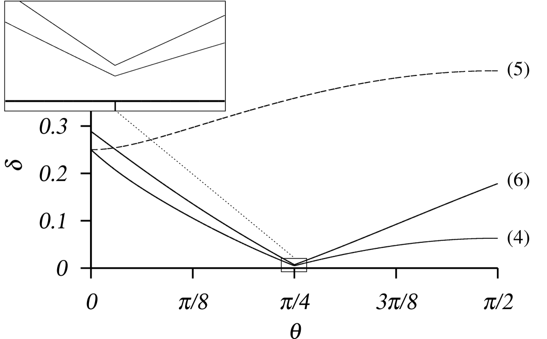
Figure 1: Example for lower and upper bounds on the optimal deviation from perfect faithfulness $\delta$ of a two state purifier with pure output. See main text for explanation.

Let us give an explicit example for these bounds. We consider the states $\rho=\frac{1}{2}({{|{0}\rangle\!\langle{0}|}}+{{|{1}\rangle\!\langle{1}|}})\otimes{{|{0}\rangle\!\langle{0}|}}$ and $\rho^{\prime}=\frac{2}{3}{{|{0}\rangle\!\langle{0}|}}\otimes{{|{+}\rangle\!\langle{+}|}}+\frac{1}{3}{{|{1}\rangle\!\langle{1}|}}\otimes{{|{\theta}\rangle\!\langle{\theta}|}}$, which appear with equal a priori probability, where ${|\theta\rangle}=\cos\theta{|0\rangle}+\sin\theta{|1\rangle}$ and ${|+\rangle}=\frac{1}{\sqrt{2}}({|0\rangle}+{|1\rangle})$. In Fig. 1 the bounds for the optimal deviation from faithfulness $\delta$ are shown: the lower bound as given in Eq. (4), the first (dashed line) and second upper bound, cf. Eq. (5) and (6). At $\theta=0$ the ranges of both states share the vector ${|1\rangle}\otimes{|0\rangle}$ and thus the worst-case distinguishability vanishes and the optimal faithfulness is given by the upper bound in Eq. (5). The second upper bound and the lower bound almost coincide at $\theta=\pi/4$ with $.0050<\delta<.0072$. Note that the upper bounds cross each other, i.e. depending on the input state, either the first or the second upper bound is tighter.

An interesting question in this context is the following: given two quantum states, does a better distinguishability (in the sense of minimum error discrimination) imply a better faithfulness? The surprising answer is no: in the example given above, the trace distance of the two states monotonically increases from $\theta=0$ to $\theta=\pi/2$, while the deviation from faithfulness has its minimum at $\theta=\pi/4$. The examples illustrates, that the worst-case distinguishability is indeed an important quantity for purifying processes. This is remarkable, as the worst-case distinguishability is purely determined by the geometric features of the states, whereas the statistical weights in the ensembles do not play any role. Note that a related, but not purely geometric quantity $F^{+}_{1}(\rho,\rho^{\prime})$ was introduced in Uhlmann (2000).

IV Sets that can be purified perfectly

Finally, our focus turns to the general analysis of perfect purifiers. The existence of a perfect purifier for a set ${\mathcal{M}}$ has far-reaching implications, as it is possible to convert all states in ${\mathcal{M}}$ to pure states in a reversible way. An investigation of the property of reversibility indeed turns out to be the key for understanding perfect purification: Suppose that we have a purifier $\Lambda$ of a set ${\mathcal{M}}$ with perfect output purity (but not necessarily perfect faithfulness), and some completely positive and trace preserving map $\Lambda^{\prime}$, such that for any $\rho_{i}\in{\mathcal{M}}$ this map is the reverse map of $\Lambda$, i.e. $\Lambda^{\prime}[\Lambda[\rho_{i}]\,]=\rho_{i}$. The action of any completely positive and trace preserving map can always be formulated as appending a (pure) ancilla state, performing a unitary rotation and finally tracing out an appropriate subsystem. We write $\Lambda^{\prime}$ in this manner and apply everything, apart from tracing out, to the output of $\Lambda$. For this composed map we write the shorthand notation $\tilde{\Lambda}$. The output of $\tilde{\Lambda}$ is still pure for any state in ${\mathcal{M}}$ and the remaining step of the map $\Lambda^{\prime}$, namely the trace over the subsystem, yields back the original state, thus $\tilde{\Lambda}$ is a perfect purifier of ${\mathcal{M}}$.

In order to further approach the characterization of sets that can be purified perfectly, we call a set of states essentially pure, if every state from the set can be globally rotated into a tensor product of a pure state and a common mixed contribution, or in more technical terms: A set of states ${\mathcal{M}}$ is called essentially pure, if one can find states $\omega_{\mathrm{aux}}$ and $\sigma_{\mathrm{B}}$, a unitary transformation $U$, and a set of pure states $\mathcal{P}_{\mathrm{A}}$, such that for all $\rho_{i}\in{\mathcal{M}}$ there is a corresponding pure state ${{|{\phi_{i}}\rangle\!\langle{\phi_{i}}|}}\in\mathcal{P}_{\mathrm{A}}$ with

$$\rho_{i}\otimes\omega_{\mathrm{aux}}=U({{|{\phi_{i}}\rangle\!\langle{\phi_{i}}|}}\otimes\sigma_{\mathrm{B}})U^{\dagger}.$$ (7)

Note, that the tensor product symbol on the two sides of this equation in general denotes different splits of the composite system: on the left hand side one sees the composition of the original system and an auxiliary system, while on the right hand side the composition refers to some system A and some system B. Essentially pure sets can be purified perfectly: A process which appends $\omega_{\mathrm{aux}}$ to $\rho_{i}$, performs $U^{\dagger}$ and traces out system B produces a pure state for any state in ${\mathcal{M}}$. On the other hand a process, which appends $\sigma_{\mathrm{B}}$ to ${{|{\phi_{i}}\rangle\!\langle{\phi_{i}}|}}$, performs $U$ and traces out the auxiliary system, undoes the action of the purifying map. Thus, a perfect purifier of ${\mathcal{M}}$ exists. Of course a union of essentially pure sets, where any two states taken from different sets are orthogonal, can also be purified perfectly. We call such a union an orthogonal union of essentially pure sets.

Theorem 2.

For a set of states ${\mathcal{M}}$, the following statements are equivalent: (i) A perfect purifier of ${\mathcal{M}}$ exists. (ii) There exists a completely positive and trace preserving map, which maps any state in ${\mathcal{M}}$ to a pure state and does not change the trace distance of any two states in ${\mathcal{M}}$. (iii) ${\mathcal{M}}$ is an orthogonal union of essentially pure sets.

Proof.

Our motivation for the definition of orthogonal unions of essentially pure sets was indeed, that this property implies the existence of a perfect purifier. Thus, we have already shown that (iii) implies (i). Furthermore, from the fact that no process can increase the trace distance, together with the existence of a reversible map, (ii) is a direct consequence of (i). Thus it only remains to show that (ii) implies (iii): If (ii) holds for an ${\mathcal{M}}$ that is a union of mutually orthogonal subsets, there exist maps that satisfy (ii) for each subset. Therefore, we can assume without loss of generality that one cannot split the set ${\mathcal{M}}$ into orthogonal parts. With ${{|{a}\rangle\!\langle{a}|}}$ being a pure auxiliary state and $U^{\dagger}$ a unitary transformation, we can write the action of $\Lambda$ as $\rho\mapsto\operatorname{tr}_{\mathrm{B}}U^{\dagger}(\rho\otimes{{|{a}\rangle\!\langle{a}|}})U$, where B denotes an appropriate subsystem. Since the output of $\Lambda$ for a state $\rho_{i}\in{\mathcal{M}}$ is a pure state (represented by a projector $\Phi_{i}$), we have $U^{\dagger}(\rho_{i}\otimes{{|{a}\rangle\!\langle{a}|}})U=\Phi_{i}\otimes\sigma_{i}$, with $\sigma_{i}$ a state in subsystem $\mathrm{B}$. The final step is now to show that $\sigma_{i}=\sigma_{j}$ holds. For any two states $\rho_{i},\rho_{j}\in{\mathcal{M}}$, due to the assumption (ii),

$${\|{\Phi_{i}-\Phi_{j}}\|}={\|{\rho_{i}-\rho_{j}}\|}={\|{\Phi_{i}\otimes\sigma_{i}-\Phi_{j}\otimes\sigma_{j}}\|}$$ (8)

holds. A minimum error discrimination Helstrom (1976); Herzog and Bergou (2004) in subsystem B at the right hand side can be written as $\sigma_{i}\rightarrow q_{i}{{|{0}\rangle\!\langle{0}|}}+(1-q_{i}){{|{1}\rangle\!\langle{1}|}}$ and $\sigma_{j}\rightarrow(1-q_{j}){{|{0}\rangle\!\langle{0}|}}+q_{j}{{|{1}\rangle\!\langle{1}|}}$, where $(q_{i}+q_{j})/2=(1+{\|{\sigma_{i}-\sigma_{j}}\|})/2$ is the success probability for the optimal discrimination measurement. We find

$$\begin{split}\|&\Phi_{i}\otimes\sigma_{i}-\Phi_{j}\otimes\sigma_{j}\|^{2}\\ &\geq({\|{q_{i}\Phi_{i}-(1-q_{j})\Phi_{j}}\|}+{\|{(1-q_{i})\Phi_{i}-q_{j}\Phi_{j}}\|})^{2}\\ &\geq{\|{\Phi_{i}-\Phi_{j}}\|}^{2}+{\|{\sigma_{i}-\sigma_{j}}\|}^{2}\,\operatorname{tr}(\Phi_{i}\Phi_{j}),\end{split}$$ (9)

where in the first step we used, that the discrimination procedure cannot increase the trace distance. The second inequality follows from a lengthy but straightforward calculation. From comparison with Eq. (8) either $\sigma_{i}=\sigma_{j}$ or $\operatorname{tr}(\Phi_{i}\Phi_{j})=0$ (or both) must hold. The latter case implies $\rho_{i}$ to be orthogonal to $\rho_{j}$, i.e. if $\sigma_{i}\neq\sigma_{j}$ for two states, then one can split ${\mathcal{M}}$ into two orthogonal sets, in contrast to our assumption. ∎

This Theorem completely characterizes all sets of states that can be purified perfectly, cf. also Eq. (7). It is surprising that one can even purify a set of continuous states, meaning that the set may contain infinitesimally close neighbors. It is also worth mentioning that all states in an essentially pure set share the same spectrum and pairwise have a completely degenerate set of canonical angles Stewart and Sun (1990). What is the lowest dimension, in which perfect purification is possible for nonorthogonal mixed states? This cannot happen unless the dimension of the Hilbert space is at least four: In two and three dimensions, only pure states can have identical spectra without having an overlapping range.

Although essentially pure sets can be characterized in a explicit manner and have a lot of straightforward features, there is no obvious method to verify whether a given set is of the structure as specified in Eq. (7). However, for the case, where ${\mathcal{M}}$ consists of only two states, there exists a computable test: From the lower bound on $\delta$ derived in equation (4) it follows that ${\|{\rho-\rho^{\prime}}\|}={\mathcal{D}({\rho},{\rho^{\prime}})}$ is a necessary condition for the existence of a perfect two-state purifier. It is also a sufficient condition: For any two states $\rho$ and $\rho^{\prime}$ there is a map $\Lambda$ such that ${\|{\Lambda[\rho]-\Lambda[\rho^{\prime}]}\|}={\mathcal{D}({\rho},{\rho^{\prime}})}$, thus if ${\|{\rho-\rho^{\prime}}\|}={\mathcal{D}({\rho},{\rho^{\prime}})}$, this map satisfies part (ii) of Theorem 2, i.e. $\rho$ and $\rho^{\prime}$ can be purified perfectly. Note, that it is also straightforward to prove that the upper bound on $\delta_{\mathrm{opt}}$ in Eq. (6) vanishes if and only if there is a perfect purifier of $\rho$ and $\rho^{\prime}$.

V Conclusions

In summary, we have introduced the concept of purification as a physical map, and studied its properties: without any prior knowledge of the input state a perfect purifier cannot exist. Relaxing one of the two characteristic properties of a purifier, purity and faithfulness, does not lead to a non-trivial universal process either. We have investigated the case when the input set contains only two states and found a characterization of the output of any map, which takes both states to a pure state. Using this tool, we derived bounds on the deviation from perfect faithfulness (i.e. the distance of the partial trace of the output state and the original state). We also completely characterized all sets of states, that can be purified perfectly. Roughly speaking, any such set can be globally rotated into a set of pure states, tensored with a common mixed contribution. Surprisingly, we found that some sets of non-commuting states can be purified, in contrast to the situation of broadcasting. For the case of sets with only two states, we provided an operational test to check whether perfect purification is possible.

In this paper we have presented some of the basic properties of purifying completely positive maps. Several questions remain open. One direction of future work is to consider the maximal possible purity of a purifier in the case of perfect faithfulness. Furthermore, the analysis of purifiers for sets with more than two states will be subject of further research.