Single-cell atomic quantum memory for light

Abstract

Recent experiments demonstrating atomic quantum memory for light [B. Julsgaard et al., Nature 432, 482 (2004)] involve two macroscopic samples of atoms, each with opposite spin polarization. It is shown here that a single atomic cell is enough for the memory function if the atoms are optically pumped with suitable linearly polarized light, and quadratic Zeeman shift and/or ac Stark shift are used to manipulate rotations of the quadratures. This should enhance the performance of our quantum memory devices since less resources are needed and losses of light in crossing different media boundaries are avoided.

I Introduction

Recently, quantum memory for light has been demonstrated in the Copenhagen lab FiurasekNature04 where the setup was almost identical to a previous experiment demonstrating long-lived entanglement of two macroscopic objects JulsgaardNature01 . Both schemes involve two cells with macroscopic numbers of cesium atoms whose spins are polarized in antiparallel directions, perpendicular to the direction of light propagation through the cells. Off-resonant interaction between the beam and the atoms causes ac Stark shift of the atomic levels and Faraday rotation of the light polarization. It has been shown that the combined effect corresponds to the quantum nondemolition (QND) interaction between atomic and light variables Kuzmich98 which can be used in many quantum information protocols Kuzmich00 . In both schemes FiurasekNature04 ; JulsgaardNature01 the two samples are placed in a homogeneous magnetic field which causes Larmor precession of the atomic spins. The reason for this is that the polarization rotation is then observed at frequency sidebands sufficiently displaced from the light frequency $\omega_{0}$, which enables us to avoid technical noises. Whereas in the entanglement scheme JulsgaardNature01 the presence of two samples was essential to demonstrate entanglement of two objects, in the memory scheme FiurasekNature04 it just helps constructing the QND Hamiltonian with the precessing spins: two light modes oscillating at frequencies $\omega_{0}+\Omega$ and $\omega_{0}-\Omega$ must be somehow matched with two atomic modes, and using two samples does the job. (Were there no technical noises, one could use directly the carrier optical frequency $\omega_{0}$ and work with a single memory cell without using magnetic field and Larmor precession.)

Although the scheme demonstrates the feasibility of a memory preserving quantum features of light pulses, it has some disadvantages. First, using two vapor cells per each stored mode increases the resources needed. Moreover, each time the light beam crosses the walls of the cell, losses occur which increase the noise. This could lead to distortion of some quantum features that then could not be recovered with sufficient fidelity. We propose here a scheme that uses a single vapor cell and still is able to involve the full QND interaction between atoms and optical signal at a sideband mode. The working medium and physical parameters chosen for the discussion are similar to those in the Copenhagen experiment FiurasekNature04 , even though the principles are valid for more general atomic systems. The important tricks are initial pumping of the atoms with a suitable linearly polarized light, and applying magnetic, optical, or microwave pulses to induce nonlinear Zeeman or Stark splitting of the atomic levels which transform the relevant quadratures.

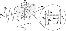
Figure 1: Geometry of the setup and scheme of the interaction in $x$ quantization. Light pulse travels in the $z$ direction, the $x$ polarization mode is in a strong coherent state and the $y$ polarization is weakly excited, carrying quantum signal. The pulse goes through atomic vapor placed in magnetic field pointing in the $x$ direction, the light being detuned from resonance of some electric dipole transition. The inset scheme illustrates the Raman transitions described by Hamiltonian (1).

II Atom-light interaction

Let us first discuss the principles of the atom-light QND interaction (see also OpatrnyFiurasek05 ). Atoms in the cell interact with light pulses traveling in the $z$ direction and with a magnetic field in the $x$ direction (see Fig. 1). The atoms are initially pumped into one of the hyperfine levels of the ground electronic state. The magnetic field $B$ causes Larmor precession of the atomic spins around the $x$ axis with frequency $\Omega\propto B$. Each pulse has a strong component which is $x$ polarized and oscillates at optical frequency $\omega_{0}=2\pi c/\lambda$ and a weak quantum component which is $y$-polarized. The atom-field interaction Hamiltonian is

$$H_{AF}=-i\hbar\sum_{m}G_{m}a_{x}\left(a_{y+}^{{\dagger}}\sigma_{m,m+1}+a_{y-}^{{\dagger}}\sigma_{m+1,m}\right)+h.c.$$ (1)

Here $a_{x}$ is the annihilation operator of the $x$ polarized photons at frequency $\omega_{0}$ off resonance of some atomic transition line, $a_{y+}^{{\dagger}}$ and $a_{y-}^{{\dagger}}$ are the creation operators of $y$ polarized photons at the sideband frequencies $\omega_{0}+\Omega$ and $\omega_{0}-\Omega$, respectively, $\sigma_{m,m^{\prime}}=|m\rangle\langle m^{\prime}|$ is the coherence between the atomic magnetic states $m$ and $m^{\prime}$ in the relevant hyperfine level with $x$ as the quantization axis. The coupling constant $G_{m}$ depends on the used isotope and particular transition. As an example, working with cesium pumped into the $F=4$ hyperfine level of the ground electronic state $6^{2}S_{1/2}$ and using light near the D2 line, the coupling is $G_{m}=\mu_{0}^{2}E_{0}^{2}/(48\hbar^{2}\Delta)\sqrt{20-m(m+1)}$, where $\mu_{0}$ is the dipole moment element of the optical transition related to the spontaneous decay rate $\gamma$ by $\mu_{0}^{2}=3\epsilon_{0}\hbar\lambda^{3}\gamma/(2\pi^{2})$, $E_{0}$ is the vacuum electric field, $E_{0}^{2}=\hbar\omega_{0}/(2\epsilon_{0}V)$, $V=AcT$ is the quantization volume, $A$ and $T$ are the transversal area and duration of the optical pulse, respectively. The detuning $\Delta$ is the frequency difference between the optical field and the given atomic D2 transition and is assumed to be much larger than the hyperfine splitting in that level and much smaller than detuning from any other atomic level. It is convenient to work with nonmonochromatic modes $a_{yC}=2^{-1/2}(a_{y-}+a_{y+})$ and $a_{yS}=2^{-1/2}(a_{y-}-a_{y+})$, whose field quadratures $X_{j}=2^{-1/2}(a_{j}+a^{{\dagger}}_{j})$, $P_{j}=-i2^{-1/2}(a_{j}-a^{{\dagger}}_{j})$ are measured using homodyne detection as the cosine and sine signal components oscillating at frequency $\Omega$. The Hamiltonian (1) is simplified when the $a_{x}$ mode is in a strong coherent state $|\alpha_{0}\rangle$ with $\alpha_{0}$ real and the atoms are initially prepared in one of the extreme states, $|F,m=-F\rangle$ or $|F,m=F\rangle$. Let us assume that atoms denoted by index 1 are initially pumped into state $|F,m=-F\rangle$ so that only the coherences $\sigma_{-F,m}$ and $\sigma_{m,-F}$ are non-negligible, and atoms denoted by index 2 are initially pumped into state $|F,m=F\rangle$ so that only the coherences $\sigma_{F,m}$ and $\sigma_{m,F}$ are non-negligible. Then after summing over all $N_{A}$ atoms of each kind, the interaction Hamiltonians for the two classes of atoms become

$$H_{\rm int}^{(1)} = \hbar\kappa(P_{C}X_{A1}+X_{S}P_{A1}),$$ (2)

$$H_{\rm int}^{(2)} = \hbar\kappa(P_{C}X_{A2}-X_{S}P_{A2}).$$ (3)

Here the atomic quadratures are defined as

$$X_{A1} = \frac{1}{\sqrt{2N_{A}}}\sum_{k=1}^{N_{A}}(\sigma^{(k)}_{-F,-F+1}+\sigma^{(k)}_{-F+1,-F}),$$ (4)

$$P_{A1} = \frac{-i}{\sqrt{2N_{A}}}\sum_{k=1}^{N_{A}}(\sigma^{(k)}_{-F,-F+1}-\sigma^{(k)}_{-F+1,-F}),$$ (5)

$$X_{A2} = \frac{1}{\sqrt{2N_{A}}}\sum_{k=1}^{N_{A}}(\sigma^{(k)}_{F-1,F}+\sigma^{(k)}_{F,F-1}),$$ (6)

$$P_{A2} = \frac{i}{\sqrt{2N_{A}}}\sum_{k=1}^{N_{A}}(\sigma^{(k)}_{F-1,F}-\sigma^{(k)}_{F,F-1}),$$ (7)

the coupling constant is $\kappa=-E_{0}^{2}\mu_{0}^{2}\sqrt{N_{L}N_{A}}/(12\hbar^{2}\Delta)$, with the photon number $N_{L}=|\alpha_{0}|^{2}$, and the index $k$ denoting individual atoms. Since for atoms 1 the populations $\sigma^{(k)}_{-F,-F}\approx 1$, and $\sigma^{(k)}_{m,m}\approx 0$ for $m\neq-F$, one can see that $X_{A1}$ and $P_{A1}$ satisfy the commutation relation $[X_{A1},P_{A1}]=i$, and similarly for atoms 2, $[X_{A2},P_{A2}]=i$.

If the light beam interacts with both classes of atoms, the total Hamiltonian $H_{\rm int}=H_{\rm int}^{(1)}+H_{\rm int}^{(2)}$ can be written as

$$H_{\rm int} = \sqrt{2}\hbar\kappa(P_{C}X_{A+}+X_{S}P_{A-}),$$ (8)

where

$$X_{A\pm} = \frac{1}{\sqrt{2}}(X_{A1}\pm X_{A2}),$$ (9)

$$P_{A\pm} = \frac{1}{\sqrt{2}}(P_{A1}\pm P_{A2}),$$ (10)

and the quadratures satisfy the cannonical commutation relations $[X_{A+},P_{A+}]=i$ and $[X_{A-},P_{A-}]=i$. The Hamiltonian (8) describes the QND interactions in two independent pairs of systems. The atomic “$+$” mode interacts with the light cosine mode and the atomic “$-$” mode interacts with the light sine mode. In contrast, each of the Hamiltonians (2) and (3) would lead to unwanted intermodal coupling of light modes C and S. Thus, with precessing spins one needs two classes of atoms to construct a QND interaction coupling one atomic mode with one light mode.

In the experiment FiurasekNature04 these two classes of oppositely polarized atoms were kept separately in two vapor cells. The initial pumping was achieved by circularly polarized light beams propagating in the $x$ direction. However, there is no principal reason why these two classes of atoms should not share the same cell. One only has to deal with a few tasks: pump the atoms into a mixture of states $|F,m=\pm F\rangle$, make sure that the coherences in atoms 1 and 2 oscillate with the same frequencies, and make sure that one can rotate the atomic quadratures of each mode on demand.

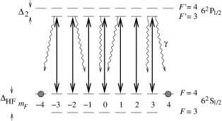
Figure 2: Scheme of the pumping process in cesium in $x$-quantization. The pump beam is linearly polarized in the $x$-direction and is resonant with the atomic transition $F=4\leftrightarrow F^{\prime}=3$. The most extreme states $|F=4,m_{F}=\pm 4\rangle$ are dark with respect to the pump. Repump field (not shown) drives the atoms out of the manifold $F=3$ so that after some time each atom ends up in one of the two dark states.

III Pumping

To prepare a mixture of both atomic classes one can use a light beam propagating in the $z$ direction, linearly polarized in the $x$ direction and tuned into resonance with the $F\leftrightarrow F^{\prime}=F-1$ transition (see Fig. 2). Light polarized along the quantization axis couples states with the same magnetic quantum number $m$ so that the two extreme states with $m=\pm F$ remain uncoupled and act as dark states with respect to the pump field. If one applies also a repump field driving the atoms out of the remaining hyperfine level (similarly as in FiurasekNature04 ; JulsgaardNature01 ), all atoms finally end up in one of the two dark states. With cesium atoms, one can drive the transition between the electronic ground state 6²S${}_{1/2},F=4$ and the excited state 6²P${}_{1/2},F^{\prime}=3$ with the D1 line 894.6 nm light.

To avoid coupling of the pumping beam to the $m=\pm F$ states, one must make sure that the pump light stays sufficiently far from resonance of the neighboring 6²P${}_{1/2},F^{\prime}=4$ state. This means that one has to take into account Doppler broadening of the transition. Fortunately, the Doppler linewidth of the room temperature cesium atoms is $\Delta_{\rm Doppler}\sim$190 MHz JulsgaardThesis03 which is much less than the hyperfine splitting of the D1 line $\Delta_{2}=$ 1168 MHz. The occupation probability of the unwanted states $m\neq\pm F$ is proportional to $\gamma\Delta_{\rm Doppler}/\Delta_{2}^{2}\approx 10^{-3}$, which is sufficiently low.

A more serious effect can stem from the fact that during collisions of oppositely polarized atoms the electrons can exchange their spins. During such a collision the atom can be brougth out of the manifold of states with $F=4$, and/or, the correlations of its coherences $\sigma_{m,m^{\prime}}$ with other atoms in the sample are averaged to zero. This effect (absent in samples with all spins oriented in the same direction) will contribute to the decoherence. Fortunately, each atom has a rather small probability $\eta$ to have such a spin exchanging collision during the relevant time $\tau$, namely $\eta\approx\sigma v\tau\rho$, where $\sigma$ is the electron spin exchange cross section (for cesium it is $\sigma\approx 2\times 10^{-14}$ cm² Beverini71 ), the density of atoms with opposite polarization is $\rho\approx 2.5\times 10^{10}$ cm^-3 and the speed is $v\approx 130$ m/s. During the interaction time $\tau=1$ ms the spin exchange collision probability is thus $\eta\approx 6.5\times 10^{-3}$. The influence on the atomic quadratures can be found following the line in Madsen04 : the quadrature mean values are shortened by a fraction $\propto\eta$ and additional fluctuation $\propto\eta$ is added to them. Since $\eta\ll 1$, states with phase-space features not finer than $\eta$ will not be seriously influenced by the spin exchanging collisions.

IV Equal oscillation frequency

In weak magnetic fields the oscillation frequency of coherences between neighboring magnetic states is nearly proportional to $B$ and independent of $m$. However, in stronger fields nonlinear Zeeman shift occurs that causes differences between the oscillation frequencies of $\sigma_{-F,-F+1}$ and $\sigma_{F-1,F}$. In particular, the difference between the neighboring energy levels is up to the second order (see, e.g., JulsgaardThesis03 ; Julsgaard04 )

$$\Omega_{Z}(m)=\frac{E_{m+1}-E_{m}}{\hbar}=\Omega_{B}-\frac{\Omega_{B}^{2}}{\Delta_{\rm HF}}(2m+1),$$ (11)

where $\Omega_{B}=\mu_{B}B/\hbar$ with $\mu_{B}$ the magnetic dipole moment and $\Delta_{\rm HF}$ is the hyperfine splitting of the ground state, which for cesium is $\Delta_{\rm HF}=2\pi\times$9.19 GHz. The difference of rotation frequencies of the two classes is $\Delta\Omega_{Z}=\Omega_{Z}(m=-F)-\Omega_{Z}(m=F-1)=14\Omega_{B}^{2}/\Delta_{\rm HF}$. Assuming the typical light pulse duration $\tau=$ 1 ms and oscillation frequency $\Omega_{B}\approx 2\pi\times 300$ kHz as in FiurasekNature04 ; JulsgaardThesis03 , one finds that the phase difference between the two coherences accumulated during the evolution would be $\Delta\Omega_{Z}\tau\approx 0.3\pi$ which is not negligible. In the double-cell scheme one can solve this problem by tuning the magnetic fields in the two cells differently so that the field difference compensates for the quadratic Zeeman shift. This cannot be done in the single cell scheme so that one has to look for another solution.

IV.1 Weak magnetic field

One option is to work with weaker magnetic fields. For example, with the Larmor frequency $\Omega_{B}\approx 2\pi\times 50$ kHz the quadratic Zeeman shift would lead to the accumulated phase difference of $\sim 20$ mrad which can be neglected. However, the laser signal on the lower-frequency sidebands can be much noisier than on higher frequencies so that one may prefer staying with stronger magnetic fields.

IV.2 Ac Stark shift

Another option is to use ac Stark shift compensating for the nonlinear Zeeman shift. We propose using suitably polarized field detuned from the D1 transitions, e.g. in cesium, 6²S${}_{1/2},F=4\leftrightarrow$ 6²P${}_{1/2},F^{\prime}=3$ and 6²S${}_{1/2},F=4\leftrightarrow$ 6²P${}_{1/2},F^{\prime}=4$. Note that the signal close to the D2 transition does not interfere with this auxiliary field. As the best candidate appears a field linearly polarized in the $x$ direction. The Stark shift of the magnetic levels is then

$$E_{S}(m)=\frac{I_{S}}{2\epsilon_{0}\hbar c}\left(\frac{|\mu_{m,m}^{(F^{\prime}=3)}|^{2}}{\Delta_{F^{\prime}=3}}+\frac{|\mu_{m,m}^{(F^{\prime}=4)}|^{2}}{\Delta_{F^{\prime}=4}}\right),$$ (12)

where the dipole moment squares are

$$|\mu_{m,m}^{(F^{\prime}=3)}|^{2} = \frac{\epsilon_{0}\hbar\lambda^{3}\gamma}{2^{7}\pi^{2}}(4-m)(4+m),$$ (13)

$$|\mu_{m,m}^{(F^{\prime}=4)}|^{2} = \frac{\epsilon_{0}\hbar\lambda^{3}\gamma}{2^{7}\pi^{2}}m^{2},$$ (14)

$\Delta_{F^{\prime}}$ is the detuning of the field with respect to the transition to the hyperfine level $F^{\prime}$, and $I_{S}$ is the Stark-shifting field intensity. If we denote by $\Delta_{S}$ the detuning of the field with respect to the center of the two $F^{\prime}=3,4$ transitions, the shift of the frequencies between the neighboring levels $\Omega_{S}(m)=[E_{S}(m+1)-E_{S}(m)]/\hbar$ is

$$\Omega_{S}(m)=\frac{\lambda^{3}\gamma I_{S}\Delta_{2}}{2^{8}\pi^{2}\hbar c}\frac{2m+1}{\Delta_{S}^{2}-\frac{\Delta_{2}^{2}}{4}}.$$ (15)

Whereas for tuning between the two D1 transitions to $F^{\prime}=3,4$, $|\Delta_{S}|<\Delta_{2}/2$, the Stark shift depends on $m$ in the same way as the quadratic Zeeman shift, for larger detunings $|\Delta_{S}|>\Delta_{2}/2$ the two shifts (11) and (15) have opposite dependences. In particular, the $m$ dependent parts of the two shifts cancel each other if the field intensity is

$$I_{S} = \frac{256\pi^{2}\hbar c\Omega_{B}^{2}}{\lambda^{3}\gamma\Delta_{\rm HF}}\left(\frac{\Delta_{S}^{2}}{\Delta_{2}}-\frac{\Delta_{2}}{4}\right).$$ (16)

When working with additional optical fields, one has to estimate their influence on atomic decoherence by photon scattering. The scattering rate of photons absorbed and spontaneously reemitted by an atom detuned by $\Delta^{\prime}$ from the photon frequency is JulsgaardThesis03 $\Gamma_{\rm ph}=\frac{\gamma}{2}\frac{s}{1+s},$ where the saturation parameter is $s=\frac{I_{S}}{I_{\rm sat}}\frac{1}{1+\left(\frac{2\Delta^{\prime}}{\gamma}\right)^{2}},$ and the saturation intensity is $I_{\rm sat}=\frac{2\pi^{2}\hbar c\gamma}{3\lambda^{3}}$. We have to integrate $\Gamma_{\rm ph}$ over $\Delta^{\prime}$ with a Gaussian distribution centered at $\Delta_{2}/2$ and having the half-width $\Delta_{\rm Doppler}$. For our values with $\Omega_{B}\approx 2\pi\times 300$ kHz and assuming $\Delta_{S}=2\pi\times 3$ GHz, the required intensity is $I_{S}\approx 1$ mW/cm² and would lead to the scattering rate of $\Gamma_{\rm ph}\approx 18$ s^-1 which is much less than the estimated scattering rate due to the probe in the Copenhagen experiments $\sim 130$ s^-1 JulsgaardThesis03 . This shows that the auxiliary field will not disturb seriously the atomic memory.

IV.3 Ac Zeeman shift

One can use microwave field tuned off-resonance with respect to the transition between the two hyperfine levels. Let us assume $\pi$-polarized field with magnetic field polarized in the $x$-direction, whose frequency is detuned by $\Delta_{\mu}$ from the hyperfine frequency $\Delta_{\rm HF}$, and whose intensity is $I_{\mu}$. The energy shift of the $m$ state is then

$$E_{\mu}(m)=\frac{I_{\mu}}{2\epsilon_{0}\hbar c^{3}\Delta_{\mu}}|\mu_{m,m}^{(\mu)}|^{2},$$ (17)

where the magnetic dipole moment element between the $m$ states of the two hyperfine levels in cesium is $\mu_{m,m}^{(\mu)}=\mu_{B}\sqrt{1-(m/4)^{2}}$, and $\mu_{B}$ is the Bohr magneton. The shift of the frequencies between the neighboring levels $\Omega_{\mu}(m)=[E_{\mu}(m+1)-E_{\mu}(m)]/\hbar$ is

$$\Omega_{\mu}(m)=\frac{I_{\mu}\mu_{B}^{2}}{32\epsilon_{0}\hbar^{2}c^{3}\Delta_{\mu}}(2m+1).$$ (18)

The ac Zeeman shift (18) compensates the nonlinear Zeeman shift (11) for the microwave field intensity

$$I_{\mu}=\frac{32\epsilon_{0}\hbar^{2}c^{3}\Delta_{\mu}\Omega_{B}^{2}}{\Delta_{\rm HF}\mu_{B}^{2}}.$$ (19)

If we use for the detuning $\Delta_{\mu}$ about ten times the frequency difference between the hyperfine transition with $m=-3$ and with $m=3$, i.e., $\Delta_{\mu}\approx 10\times 12\Omega_{B}=2\pi\times 36$ MHz, the intensity with $\Omega_{B}=2\pi\times 300$ kHz should be $I_{\mu}\approx 1.4$ W/cm².

V Quadrature rotations

Although the above discussion shows the availability of the QND Hamiltonian (8), to be useful as a quantum memory medium, one has to be able to manipulate to some extent the atomic degrees of freedom. An important operation is rotation of the atomic quadratures of each mode Kuzmich00 , in our case, e.g., $P_{A+}\to X_{A+}$ and $X_{A+}\to-P_{A+}$, and similarly for the “$-$” mode. In the two-cell schemes this is achieved by magnetic pulses acting separately on each atomic sample. For example, a magnetic $\pi/2$ pulse in one cell causes the Zeeman shift yielding the rotation $P_{A1}\to X_{A1}$ and $X_{A1}\to-P_{A1}$. However, oppositely oriented magnetic $\pi/2$ pulse in the other cell would cause the corresponding rotation $P_{A2}\to X_{A2}$ and $X_{A2}\to-P_{A2}$ which would lead to the desired transformation of $X_{A+}$ and $P_{A+}$. The definition of the collective quadratures $X_{A2}$ and $P_{A2}$ in (6) and (7) means that these quadratures would respond oppositely in weak magnetic fields in comparison to $X_{A1}$ and $P_{A1}$, i.e., $P_{A2}\to-X_{A2}$ and $X_{A2}\to P_{A2}$. Thus, if one used the same weak magnetic pulse for the two classes of atoms in the same cell, the two atomic modes would mix: $P_{A+}\to X_{A-}$, $X_{A+}\to-P_{A-}$, and $P_{A-}\to X_{A+}$, $X_{A-}\to-P_{A+}$.

To solve this problem one can take advantage of the frequency difference of the coherences $\sigma_{-F,-F+1}$ and $\sigma_{F-1,F}$ caused by the nonlinear stationary Zeeman effect, by the ac Stark shift, and/or by the ac Zeeman shift.

V.1 Nonlinear Zeeman shift

When using the nonlinear Zeeman effect, one can apply a sufficiently strong magnetic field for a short time. During the magnetic pulse atoms complete many 2$\pi$ rotations, however atoms in the $m=-F$ class would end up half a rotation ahead in comparison to those in the $m=+F$ class. To achieve this, one can use a magnetic pulse of duration $\tau$ such that $\Delta\Omega\tau=\pi$. If the time is chosen $\tau\approx 30$ $\mu$s (i.e., much shorter than the 1 ms reading and writing pulses), one finds that the linear frequency should be $\Omega_{B}\approx 2\pi\times 3.1$ MHz corresponding to $B\approx 8.8$ G. Although feasible in principle, it can be technically rather challenging to produce such strong, precisely controlled, short magnetic pulses.

V.2 Ac Stark shift

Another option is to apply a Stark-shifting optical pulse, similarly as in the preceding paragraphs. The field produces state-dependent energy shift leading to increased frequency difference of the coherences $\sigma_{-F,-F+1}$ and $\sigma_{F-1,F}$. When the pulse duration is $\tau$, the field intensity should be such that $\left|\Omega_{S}(m=F-1)-\Omega_{S}(m=-F)\right|\tau=\pi$. Using Eq. (15) for a $\pi$ polarized pulse, one finds the condition

$$I_{S}=\frac{32\pi^{3}\hbar c}{7\lambda^{3}\gamma\tau}\frac{|\Delta_{2}^{2}-4\Delta_{S}^{2}|}{\Delta_{2}}\approx\frac{128\pi^{3}\hbar c\Delta_{S}^{2}}{7\lambda^{3}\gamma\Delta_{2}\tau},$$ (20)

where the approximation is valid for $|\Delta_{S}|\gg\Delta_{2}/2$. As an example, let us consider $\Delta_{S}=2\pi\times 3$ GHz and $\tau=30~{}\mu$s, which would require field intensity $I_{S}\approx$ 135 mW/cm². The number of scattered photons is in this case $n_{\rm phot}\approx 0.06$ which is smaller than the number of photons scattered from the information carrying pulses $\sim 0.1$. Note that when increasing the detuning and field intensity, the number of scattered photons approaches its limit $n_{\rm phot}\to 24\pi/7\times\gamma/\Delta_{2}\approx 0.04$.

V.3 Ac Zeeman shift

When a source of suitably polarized microwave field is available, one can take advantage of the $m$ dependence of the ac Zeeman shift as in Eq. (18). If a $\pi$ phase difference between the two atomic classes is to be achieved during time $\tau$, one needs the microwave field intensity

$$I_{\mu}=\frac{16\pi\epsilon_{0}\hbar^{2}c^{3}\Delta_{\mu}}{7\mu_{B}^{2}\tau}.$$ (21)

Assuming as in the preceding section $\Delta_{\mu}\approx 2\pi\times 36$ MHz and $\tau=30\ \mu$s we get the required microwave field intensity $I_{\mu}\approx$ 170 W/cm².

VI Conclusion

We have shown how a single atomic vapor cell can be used as a quantum memory for light with the quantum signal encoded at two sideband frequencies. The sideband encoding is required so as to suppress technical noises that would occur if one measures the light signal by integration of the cw homodyne signal over the pulse duration (typically a millisecond). The two sideband modes must be matched by two atomic modes; we have shown how to use two atomic coherences in one sample rather than using one cell for each atomic mode.

The single-cell approach could substantially reduce the losses of light occurring at the boundaries between different media (air, paraffin coated glass walls of the cells, atomic vapor) and save the resources needed. The losses would be especially disturbing if squeezed states are to be manipulated: absorption of ${\cal A}$ at each boundary would add $\sim{\cal A}$ of vacuum noise to the signal. Thus, with small losses ${\cal A}\ll 1$, if a beam with a perfectly squeezed quadrature crosses four boundaries (when working with the double-cell scheme), the noise added to the squeezed quadrature would be twice as big as when crossing two boundaries (single cell scheme).

The scheme requires selective addressing of atoms in the $m=-F$ and $m=+F$ manifolds, which react differently to strong stationary magnetic fields (nonlinear Zeeman effect), to Stark-shifting optical pulses, or to microwave fields (ac Zeeman shift). Experimentalists will have to find the best combination of these approaches to trade-off between their advantages and disadvantages. When applied, the scheme should enhance our capabilities of storing and processing quantum information carried by light.

- (1) B. Julsgaard, J. Sherson, J. I. Cirac, J. Fiurášek, and E. S. Polzik Nature 432, 482 (2004).
- (2) B. Julsgaard, A. Kozhekin, and E.S. Polzik, Nature 413, 400 (2001).
- (3) A. Kuzmich, N.P. Bigelow, and L. Mandel, Europhys. Lett. 42, 481 (1998); A. Kuzmich et al., Phys. Rev. A 60, 2346 (1999); K. Mølmer, Eur. Phys. J. D 5, 301 (1999); Y. Takahashi et al., Phys. Rev. A 60, 4974 (1999).
- (4) A. Kuzmich and E.S. Polzik, Phys. Rev. Lett. 85, 5639 (2000); L.M. Duan et al., ibid 85, 5643 (2000); A. Di Lisi and K. Mølmer, Phys. Rev. A 66, 052303 (2002); S. Massar and E.S. Polzik, Phys. Rev. Lett. 91, 060401 (2003); J. Fiurášek, Phys. Rev. A 68, 022304 (2003); A. Kuzmich and T.A.B. Kennedy, Phys. Rev. Lett. 92, 030407 (2004); J. Fiurášek et al., ibid 93, 180501 (2004); K. Hammerer et al., Phys. Rev. A 70, 044304 (2004).
- (5) T. Opatrný and J. Fiurášek, Phys. Rev. Lett. 95, 053602 (2005).
- (6) B. Julsgaard, Entanglement and quantum interactions with macroscopic gas samples, Ph.D. thesis, Aarhus University, Denmark (2003, available at www.nbi.dk/julsgard/).
- (7) N. Beverini, P. Minguzzi, and Strumia, Phys. Rev. A 4, 550 (1971). Note that this cross section was measured by monitoring the decay of the spin in a spin polarized sample, and may therefore not be directly applicable here. We can expect however, that the relevant cross section is of similar magnitude.
- (8) L. B. Madsen and K. Mølmer, Phys. Rev. A 70, 052324 (2004).
- (9) B. Julsgaard, J. Sherson, J.L. Sørensen, and E.S. Polzik, J. Opt. B: Quantum Semiclas. Optics 6, 5 (2004).