Description of Quantum Entanglement with Nilpotent Polynomials

Abstract

We propose a general method for introducing extensive characteristics of quantum entanglement. The method relies on polynomials of nilpotent raising operators that create entangled states acting on a reference vacuum state. By introducing the notion of tanglemeter, the logarithm of the state vector represented in a special canonical form and expressed via polynomials of nilpotent variables, we show how this description provides a simple criterion for entanglement as well as a universal method for constructing the invariants characterizing entanglement. We compare the existing measures and classes of entanglement with those emerging from our approach. We derive the equation of motion for the tanglemeter and, in representative examples of up to four-qubit systems, show how the known classes appear in a natural way within our framework. We extend our approach to qutrits and higher-dimensional systems, and make contact with the recently introduced idea of generalized entanglement. Possible future developments and applications of the method are discussed.

year number number identifier Date text ]

LABEL:FirstPage1

I Introduction: How to characterize entanglement?

Inseparability of quantum states of composite systems, discovered in the early days of quantum mechanics by A. Einstein, B. Podolsky, and N. Rosen Einstein and named “entanglement” (“Verschränkung”) by E. Schrödinger Schrodinger , became one of the central concepts of contemporary physics during the last decade. Entanglement plays now a vital role within quantum information science QI , representing both the defining resource for quantum communication – where it enables, in particular, non-classical protocols such as quantum teleportation Braunstein and it leads to enhanced security in cryptographic tasks Cryptography – and a key ingredient for determining the efficiency of quantum algorithms and quantum computation schemes Josza ; Orus . In addition, studies of entanglement have also proved be relevant to fields as different as atomic physics Gershon , quantum chaos Dima ; Casati ; Santos ; Montangero , quantum phase transitions Arnesen ; Osborne ; Vidal ; Eryigit ; Stelmachovi ; Amico ; Somma ; Chei , and quantum networks Cubitt .

According to the original definition, the description of entanglement relies on a specific partition of the composite physical system under consideration. However, such a system can often be decomposed into a number of subsystems in many different ways, each of the subsystems possibly being a composite system by itself. In order to avoid ambiguity, given a partition of the composite system into $n$ subsystems, we call each of them an “element” and characterize it by a single, possibly collective, quantum number. Thus, the composite system is a collection of the elements. We call this collection an “assembly” in order to avoid confusion with an “ensemble”, which is usually understood as a set of all possible realizations of a many-body system with an associated probability distribution over these realizations. The $i$-th element is assumed to have Hilbert space of dimension $d_{i}$. Qubit, qutrit, and qudit are widely used names for two-, three-, and $d$-level elements (with $d_{i}=2$, $d_{i}=3$, and $d_{i}=d$, respectively).

The term “entanglement” has a transparent qualitative meaning: A pure state of an assembly is entangled with respect to a chosen partition when its state vector cannot be represented as a direct product of state vectors of the elements. This notion can also be extended to generic mixed quantum states, whereby entanglement is defined by the inability to express the assembly density operator as a probabilistic combination of direct products of the density operators of the elements. Intuitively, one expects that in the presence of “maximum” entanglement Zeilinger , the states of all subsystems comprising the overall system are completely correlated in such a way that a measurement performed on one part determines the states of all other parts.

The question is: how to quantitatively characterize entanglement for an assembly of many elements? One would like to have a measure ranging from zero for the product state to the maximum value for the maximally entangled state. This can be easily accomplished for the bipartite setting $n=2$ that is, for an assembly consisting just of two distinguishable elements $A$ and $B$, each of arbitrary dimension. In this case, the von Neumann $\mathrm{Tr}[\rho_{A}\log\rho_{A}]$ or linear $\mathrm{Tr}[\rho_{A}^{2}]$ entropies based on the reduced density operator of either element, e.g., $\rho_{A}=\mathrm{Tr}_{B}[\left|\Psi\right\rangle\left\langle\Psi\right|]$, may be chosen as entanglement measures for a pure state $\left|\Psi\right\rangle$ of the assembly. However, already for the tripartite case $n=3$, characterizing and quantifying entanglement becomes much harder. In fact, there are not one, but many different characteristics of entanglement and, apart from the question “How much?”, one has also to answer the question “In which way” Dur ; Verstraete are different elements entangled? In other words, apart from separability criteria Peres , one also has to introduce inequivalent entanglement measures Wootters ; Vedral ; Meyer ; Wong ; Rungta ; Bennett ; Heydari and entanglement classes Verstraete2 ; Dur ; Acin ; Akimasa .

The identification of appropriate measures is not unique, and is mostly dictated by convenience. The choice of classes may have a more solid ground based on group theory, since their definition is related to groups of local operations. These are operations applied individually to each of the elements and forming a subgroup of all possible transformations of the assembly state vector. One may resort to group-theoretical methods, which allow one to construct a set of invariants Verstraete2 ; Grassl ; Barnum ; Leifer under such local operations. Under the action of local transformations, which can be either unitary or, in the most general case, simply invertible, the state vector of the system undergoes changes, still remaining within a subset $\mathcal{O}$ (an orbit) of the overall Hilbert space $\mathcal{H}$. The dimension of the coset $\mathcal{H}/\mathcal{O}$, that is the number of independent invariants identifying the orbit, can be easily found for a generic quantum state. Still, there are singular classes of orbits that require special consideration. Their description depends critically on the number of elements and on the detailed structure of the assembly.

The numerical values of the complete set of invariants may be chosen as the “orbit markers” that provide one with an entanglement classification, although the choice of this set is not, in general, unique. It turns out that generally accepted measures of entanglement, such as concurrence Wootters for two qubits ($n=2$, $d_{i}=2$), and $3$-tangle Dur for three qubits ($n=3$, $d_{i}=2$), are such invariants Verstraete2 ; Gingrich . Generalization of these measures Verstraete2 to $n=4$, $d_{i}=2$ provides a connection between measures and invariants characterizing different classes. Their construction is not an easy task, and one needs to identify the invariants that are able to distinguish inequivalent types of entanglement Osterloh . Moreover, the invariants are usually high-order polynomials of the state amplitudes, with the maximum power growing linearly with the number of elements in the assembly. Therefore they rapidly become rather awkward Leifer ; MLV . A partial albeit not unambiguous connections between the measures and classes are established by the requirement Vidal2 for a measure to behave as a so-called monotone. This means it should be non-increasing on average under the action of non-unitary invertible transformations of the elements, also known as the family of Local Operations and Classical Communication, LOCC Bennett2 . The complete classification problem remains unsolved even for relatively small assemblies (see e.g. Luque for recent results on the the five-qubit system).

Apart from polynomial-invariant constructions, other schemes have been proposed to describe multipartite entanglement, including those based on generalization of Schmidt decomposition Acin ; Carteret2 ; Brun ; Sudbery , on invariant eigenvalues Verstraete2 , on hyperdeterminants Akimasa , and on expectation values of anti-linear operators Osterloh . However, none of these suggestion has been fully tested for $n>4$ qubits or more than three qutrits ($n>3$, $d=3$) Briand . Moreover, for the orbits of general invertible local transformations, the complete sets of invariants are unknown Kac for assemblies consisting of $n$ qudits ($d_{i}=d$) if $n>3$ and/or $d>4$. Still, a number of physically reasonable suggestions Meyer ; Heydari ; Stockton ; Linden for entanglement characterization have been attempted.

In this paper, we propose a different approach to entanglement characterization. We focus exclusively on the case where an assembly in a pure quantum state consists of distinguishable elements, leaving generalizations to mixed states and to indistinguishable elements for future studies. Our main aim is to construct extensive characteristics of entanglement. Thermodynamic potentials linearly scaling with the number of particles in the system offer examples of extensive characteristics widely employed in statistical physics. The free energy given by the logarithm of the partition function is a specific important example. We will introduce similar characteristics for entangled states in such a way that their values for a product state coincide with the sum of the corresponding values for unentangled groups of elements. This technique is based on the notion of nilpotent variables and functions of these variables. An algebraic variable $x$ is called nilpotent if an integer $n$ exists such that $x^{n}=0$. In our case, these variables are naturally provided by creation operators, whence the logarithm function transforming products into sums plays the central role in the construction.

Our approach is based on three main ideas: (i) We express the state vector of the assembly in terms of a polynomial of creation operators for elements applied to a reference product state. (ii) Rather than working with the polynomial of nilpotent variables describing the state, we consider its logarithm, which is also a nilpotent polynomial. Due to the important role that this quantity will play throughout the development, we call this quantity the nilpotential henceforth, by analogy to thermodynamic potentials. (iii) The nilpotential is not invariant under local transformations, being different in general for different states in the same orbit. We therefore specify a canonic form of the nilpotential to which it can be reduced by means of local transformations. The nilpotential in canonic form is uniquely defined and contains complete information about the entanglement in the assembly. We therefore call this quantity the tanglemeter. The latter is, by construction, extremely convenient as an extensive orbit marker: the tanglemeter for a system consists of several not interacting, unentangled groups of elements equals the sum of tanglemeters of these groups.

Let us briefly explain these ideas, in the simplest example of $n$ qubits, which will be discussed in detail in Sect. II. An assembly of $n$ qubits is subject to the $su(2)_{1}\oplus\ldots\oplus su(2)_{i}\ldots\oplus su(2)_{n}$ Lie algebra of local transformations note0 . As a reference state, we choose the Fock vacuum that is, the state $\left|\mathrm{O}\right\rangle=\left|0,0,\ldots,0\right\rangle$ with all the qubits being in the ground state. An arbitrary state of the assembly may be generated via the action of a polynomial $F(\sigma_{i}^{+})$ in the nilpotent operators $\sigma_{i}^{+}$ on the Fock vacuum. Here, the subscript $i$ enumerates the qubits, and the operator $\sigma_{i}^{+}$ creates the state $|1\rangle$ out of the state $|0\rangle$. Evidently, $(\sigma_{i}^{+})^{2}=0$, since the same quantum state cannot be created twice. The family of all polynomials $F(\sigma_{i}^{+})$ forms a ring. We note that anticommuting nilpotent (Grassmann) variables are widely employed in quantum field theory Berezin and in condensed matter physics Efetov . However, the nilpotent variables introduced here commute with one another.

In order to uniquely characterize entanglement, one must first select a convenient orbit marker. Following the idea of Ref. Carteret2 , we take as such a state $\left|\Psi_{c}\right\rangle_{\mathcal{O}}$ lying in the orbit $\mathcal{O}$, which is the “closest” to the reference state $\ \left|\mathrm{O}\right\rangle$ in the inner product sense, that is $\left|\left\langle\mathrm{O}\right.\left|\Psi_{c}\right\rangle_{\mathrm{O}}\right|=\max$. Once the state $\left|\Psi_{c}\right\rangle_{\mathrm{O}}$ is found, it is convenient to impose a non-standard normalization condition $\left|\left\langle\mathrm{O}\right.\left|\Psi_{c}\right\rangle_{\mathrm{O}}\right|=1$. We call the resulting state $\left|\Psi_{c}\right\rangle_{\mathrm{O}}$ canonic. The canonic state is associated with the canonic form of the polynomial $F_{c}(\sigma_{i}^{+})$, which begins with a constant term equal to $1$.

We mainly work not with $F_{c}$ by itself, but with the tanglemeter – a nilpotent polynomial $f_{c}=\ln F_{c}$ that can be explicitly evaluated by casting the logarithm function in a Taylor series of the nilpotent combination $F_{c}-1$. Since $(\sigma_{i}^{+})^{2}=0$, this series is a polynomial containing at most $2^{n}$ terms. Both the tanglemeter and nilpotential ($f=\ln F$) resemble to the eikonal, which is the logarithm of the regular semi-classical wave function in the position representation, multiplied by $-i$. The difference is that in our case no approximation is made: $f$ represents the logarithm of the exact state vector.

The nilpotential $f$ and the tanglemeter $f_{c}$ have several remarkable properties: (i) the tanglemeter provides a unique and extensive characterization of entanglement; (ii) a straightforward entanglement criterion can be stated in terms of the cross derivatives $\partial^{2}f$/$\partial\sigma_{i}^{+}\partial\sigma_{j}^{+}$; (iii) the dynamic equation of motion for $f$ can be written explicitly and, suggestively, in the rather general case has the same form as the well-known classical Hamilton-Jacobi equation for the eikonal.

The paper is organized as follows. In Sect. II, we analyze in detail an assembly of $n$ qubits in terms of the nilpotent polynomials $F$ and $f$. We extend the notion of canonic forms to the group of reversible local transformations $SL(2,\mathbb{C})$ and introduce the idea of entanglement classes. We conclude the section by presenting expressions relating the coefficients of $F_{C}$ and $f_{C}$ with known measures of entanglement. To avoid confusion, we note that the subscript $c$ corresponds to $su$-canonic forms in contrast to $C$, which corresponds to $sl$-canonic forms. Details of the calculations and some proofs are given in Appendices A and B along with graphic representations of the entanglement topology.

In Sect. III, we consider the evolution of the nilpotent polynomials under the action of single-qubit and two-qubit Hamiltonians, and derive an equation of motion for the nilpotential, which is distinct from the Schrödinger equation. For one important particular case able to support universal quantum computation Barenco , we show that this equation has a form of the classical $n$-dimensional Hamilton-Jacobi equation. Describing quantum dynamics in terms of nilpotentials suggests a computational algorithm for evaluating tanglemeters, which can be performed by dynamically reducing the polynomials to the forms canonic under either $SU(2)$ or $SL(2,\mathbb{C})$ local transformations. In the example of a four-qubit assembly, we explicitly illustrate how to identify the resulting entanglement classes. This technique yields entanglement classes consistent with the results of Ref. Verstraete . The explicit analysis of these classes as well as details of derivation of the equation of motion are given in Appendices B and C.

In Sect. IV, we extend our technique to assemblies of $d$-level elements – starting from qutrits Cereceda ; CHSH . The Cartan-Weyl decomposition of the $su(d)$ algebras suggests a natural choice of nilpotent variables for qudits. For each element, we have $d-1=r$ variables representing commuting root vectors from the corresponding Lie algebra, which has rank $r$. For the illustrative case of two and three qutrits, we discuss possible choices of the canonic forms of the nilpotent polynomials. We further extend the approach to the case where the assembly partition may change as a result of the merging of elements, such that the new assembly consists of fewer number of elements with $d_{i}\neq d_{j}$, and consider transformations of nilpotent polynomials associated with such a change. Finally, we address a situation encountered in the framework of generalized entanglement Barnum1 ; Barnum2 , where the rank $r$ of the algebras of allowed local transformations is less than $d-1$. In other words, while the assembly is still assumed to be composed of a number of distinct elements, the group of local operations need not involve all possible local transformations. In such a situation, the proper nilpotent variables are more complicated than $\sigma^{+}$. In particular, they may have non-vanishing squares etc, with only $d_{i}$ powers vanishing. In addition, unlike in the conventional setting, entanglement relative to the physical observables may exist not only among different subsystems, but also within a single element.

We conclude by summarizing our results and discussing possible developments and future applications of nilpotent polynomials and the tanglemeter.

II Entanglement characterization via nilpotent polynomials

Consider $n$ qubits in a generic pure state $|\Psi\rangle$,

$$\left|\Psi\right\rangle =\sum_{\left\{k_{i}\right\}={0,1}}\psi_{k_{n}k_{n-1}\ldots k_{1}}\left|k_{n},k_{n-1},\ldots,k_{1}\right\rangle=\psi_{00\ldots 0}\left|0,0,\ldots 0\right\rangle$$

$$+\psi_{10\ldots 0}\left|1,0,\ldots 0\right\rangle+\psi_{01\ldots 0}\left|0,1,\ldots 0\right\rangle+\ldots+\psi_{11\ldots 1}\left|1,1,\ldots 1\right\rangle\>,$$ (1)

specified by $2^{n}$ complex amplitudes $\psi_{k_{n}k_{n-1}\ldots k_{1}}$, i.e. by $2^{n+1}$ real numbers. The index $k_{i}=0,1$ corresponds to the ground or excited state of the $i$-th qubit, respectively. When we take normalization into account and disregard the global phase, there are $2^{n+1}-2$ real parameters characterizing the assembly state.

It is natural to expect that any measure characterizing the intrinsic entanglement in the assembly state remains invariant under unitary transformations changing the state of each qubit. A generic $SU(2)$ transformation is the exponential of an element of the $su(2)$ algebra,

$$U=\exp[\mathrm{i}(\sigma^{x}P^{x}+\sigma^{y}P^{y}+\sigma^{z}P^{z})]\ ,$$ (2)

where $\sigma^{x}$, $\sigma^{y}$, and $\sigma^{z}$ are Pauli matrices. It depends on the three real parameters $P^{x}$, $P^{y}$, and $P^{z}$. Such a transformation changes the amplitudes $\psi_{k_{n}k_{n-1}\ldots k_{1}}$ in Eq. (1), but preserves some combinations of these amplitudes – the invariants of local transformations. Thus, local transformations move the state along an orbit $\mathcal{O}$, while the values of the invariants serve as markers of this orbit.

The first relevant question is: What is the maximum number of real invariants required for the orbit identification, hence, for entanglement characterization? A generic $SU(2)$ transformation represented by Eq. (2) depends on three real parameters. Therefore, for $n$ qubits the dimension of the coset $\mathcal{H}/\mathcal{O}$, that is the number of different real parameters invariant under local unitary transformations, reads Linden ; Carteret2

$$D_{su}=2^{n+1}-3n-2\ .$$ (3)

Mathematically, the counting in Eq. (3) corresponds to the number of the invariants of the group $\otimes_{i}SU_{i}(2)\otimes U(1)$, where the factor $U(1)$ describes the multiplication of the wave function on the common phase factor and the usual normalization condition $\langle\Psi|\Psi\rangle=1$ for the wave function is imposed. It is more convenient for us to reformulate the same problem as seeking for the invariants of $\otimes_{i}SU_{i}(2)\otimes\mathbb{C}^{*}$, where $\mathbb{C}^{*}$ is the group of multiplication by an arbitrary nonzero complex number and no normalization condition on the wave function is imposed. This will allow us to choose a representative on the orbit of $\mathrm{O}$ with nonstandard normalization choice $\langle\Psi_{C}|\mathrm{O}\rangle=1$.

To be precise, the counting Eq. (3) is true for $n>2$ while the case $n=2$ is special: in spite of the fact that $2^{3}-3\cdot 2-2=0$, there is a nontrivial invariant of local transformations for two qubits. It has the form

$$I\ =\ \psi_{00}\psi_{11}-\psi_{01}\psi_{10}.$$ (4)

For a three-qubit system, five independent local invariants exist Gingrich , namely three real numbers

$$I_{1} =\psi_{kij}\psi^{\ast pij}\psi_{pmn}\psi^{\ast kmn}\ ,$$

$$I_{2} =\psi_{ikj}\psi^{\ast ipj}\psi_{mpn}\psi^{\ast mkn\ },$$

$$I_{3} =\psi_{ijk}\psi^{\ast ijp}\psi_{mnp}\psi^{\ast mnk\ },$$ (5)

and the real and the imaginary part of a complex number,

$$I_{4}+\mathrm{i}I_{5}=\psi_{ijk}\psi^{ijp}\psi_{mnp}\psi^{mnk}.$$ (6)

Here, $\psi^{ijk}=\epsilon^{ii^{\prime}}\epsilon^{jj^{\prime}}\epsilon^{kk^{\prime}}\psi_{i^{\prime}j^{\prime}k^{\prime}}$, with the summation over repeated indexes taking values $0$ and $1$ implicit, $\psi^{\ast}{}^{ijk}$ denotes the complex conjugate of $\psi_{ijk}$, and $\epsilon^{ii^{\prime}}$ is the antisymmetric tensor of rank $2$. The quantity $2|I_{4}+iI_{5}|$ is also known by the name residual entanglement or 3-tangle $\tau$ Refs. Wong ; Akhtarshenas .

Similar invariants can still be found for a four-qubit system. However, with increasing $n$, the explicit form of the invariants becomes less and less tractable and convenient for practical use. Moreover, no explicit physical meaning can be attributed to such invariants. We therefore suggest an alternative way to characterize entanglement, which is based on: (i) Specifying the canonic form of the state that unambiguously marks an orbit; (ii) Characterizing this state with the help of coefficients of a nilpotent polynomial; (iii) Considering the logarithm of this polynomial, the tanglemeter. Thus, we construct extensive invariants of local transformations as the coefficients of the tanglemeter that is, nilpotential of the canonic state.

In this section, we proceed with illustrating the main technical advantages of our description within the qubit setting, deriving an entanglement criterion, and explaining how the invariants constructed by our method are related to existing entanglement measures. We also analyze a case important for certain applications involving indirect measurements, where it is natural to consider a broader class of local transformations constrained only by the requirement of unit determinant. Specifically, we focus on the set of stochastic local operations assisted by classical communication Bennett2 , which is widely employed in quantum communication studies and protocols. For qubits, such transformations are known as SLOCC maps Bennett . These operations do not necessarily preserve the normalization of state vectors. However, as suggested by Theorem 1 of Ref. Verstraete2 , after a proper renormalization they are described by the complexification $sl(2,\mathbb{C})$ of the $su(2)$ algebra, such that the parameters $(P_{i}^{x},P_{i}^{y},P_{i}^{z})$ specifying the transformation of Eq. (2) on each qubit are now complex numbers. The corresponding real positive invariants of local $SL(2,\mathbb{C})$ transformations are monotones.

II.1 Canonic form of entangled states

In order to unambiguously attribute a marker to each orbit, we specify a canonic form of an entangled assembly state. To this end, we first identify a reference state $\left|\mathrm{O}\right\rangle$ as a direct product of certain one-qubit states. The latter can be chosen in an arbitrary way, but the choice $|0\rangle$, with the lowest energy level occupied, is the most convenient to our scope. Thus, the reference state reads $\left|\mathrm{O}\right\rangle\ =\ |0,\ldots 0\rangle$. Drawing parallels with quantum field theories and spin systems, we will call $\left|\mathrm{O}\right\rangle$ the “ground” or “vacuum” state. Then, following a suggestion of Ref. Carteret2 , by applying local unitary operations to a generic quantum state $\left|\Psi\right\rangle$, we can bring it into the “canonic form” $\left|\Psi_{c}\right\rangle$ corresponding to the maximum possible population of the reference state $\left|\mathrm{O}\right\rangle$. In other words, we apply a direct product $U_{1}\otimes\ldots\otimes U_{n}$ of transformations as in Eq. (2) to the state vector $\left|\Psi\right\rangle$, and choose real parameters $(P_{i}^{x},P_{i}^{y},P_{i}^{z})$ to maximize $\left|\left\langle\mathrm{O}\right|U_{1}\otimes\ldots\otimes U_{n}\left|\Psi\right\rangle\right|^{2}$. The transformation $U_{1}\otimes\ldots\otimes U_{n}$ satisfying this requirement can be seen to be unique up to phase factors multiplying the upper states of each qubit. Modulo this uncertainty, the canonic state $\left|\Psi_{C}\right\rangle=U_{1}\otimes\ldots\otimes U_{n}\left|\Psi\right\rangle$ can serve as a valid orbit marker.

In fact, a generic unitary transformation of the $m$-th qubit, chosen in the form $\exp[\mathrm{i}\sigma^{z}\phi_{m}]$ $\exp[\mathrm{i}\sigma^{x}g_{m}]$ $\exp[\mathrm{i}\sigma^{z}\varphi_{m}]$, $\phi_{m},g_{m},\varphi_{m}\in\mathbb{R}$, equivalent to Eq. (2), results in

$$\psi_{\ldots k_{m}=0\ldots} \rightarrow\psi_{\ldots k_{m}=0\ldots}\mathrm{e}^{-\mathrm{i}\phi_{m}-\mathrm{i}\varphi_{m}}\cos g_{m}+\mathrm{i}\psi_{\ldots k_{m}=1\ldots}\mathrm{e}^{\mathrm{i}\varphi_{m}-\mathrm{i}\phi_{m}}\sin g_{m},$$

$$\psi_{\ldots k_{m}=1\ldots} \rightarrow\psi_{\ldots k_{m}=1\ldots}\mathrm{e}^{\mathrm{i}\phi_{m}+\mathrm{i}\varphi_{m}}\cos g_{m}+\mathrm{i}\psi_{\ldots k_{m}=0\ldots}\mathrm{e}^{\mathrm{i}\phi_{m}-\mathrm{i}\varphi_{m}}\sin g_{m}.$$ (7)

Let us consider a generic infinitesimal local transformation of the state in the canonic form. By expanding Eq. (7) in series in $g_{m}$ up to the second order, one obtains

$$\left\langle\mathrm{O}\Big{|}\otimes_{i}U_{i}\Big{|}\Psi\right\rangle\rightarrow{\bigg{[}}\Big{(}1-\sum\limits_{m}\tfrac{g_{m}^{2}}{2}\Big{)}\psi_{0\ldots 0}+\mathrm{i}\sum_{m}g_{m}\mathrm{e}^{2\mathrm{i}\varphi_{m}}\psi_{0\ldots k_{m}=1\ldots 0}-\sum_{m>l}g_{m}g_{l}\mathrm{e}^{2\mathrm{i}(\varphi_{m}+\varphi_{l})}\psi_{0\ldots k_{m}=1\ldots k_{l}=1\ldots 0}{\bigg{]}}\prod\limits_{r}\mathrm{e}^{-\mathrm{i}(\phi_{r}+\varphi_{r})}\,,$$ (8)

for the amplitude of the ground state. Since the parameters of the transformation are arbitrary, the condition of maximum ground-state population $\left|\left\langle\mathrm{O}|\Psi\right\rangle\right|^{2}$ implies that the linear term in Eq. (8) vanishes,

$$\psi_{0\ldots k_{m}=1\ldots 0}=0\>,\;\;\;\forall m\>.$$ (9)

This gives $n$ complex conditions and implicitly specifies $2n$ out of $3n$ real parameters of the local transformation that maps a generic state to the canonic form. The remaining $n$ parameters may be identified in a generic case with the phase factors $\mathrm{e}^{-\mathrm{i}(\phi_{r}+\varphi_{r})}$, where one can set $\phi_{r}=0$ without loss of generality. Two remarks are in order.

(i) Special families of states of measure zero in the assembly Hilbert space may exist for which the system of equations (9) is degenerate and specifies less than $2n$ parameters. The simplest example for $n=2$ is the Bell state, with $\psi_{00}=\psi_{11}=1/\sqrt{2}$ and $\ \psi_{01}=\psi_{10}=0$. The combination of two transformations of the form (7) gives a state with the amplitudes

$$\psi^{\prime}_{00}\ =\ \frac{e^{-\mathrm{i}(\phi_{1}+\phi_{2})}}{\sqrt{2}}\left[e^{-\mathrm{i}(\varphi_{1}+\varphi_{2})}\cos g_{1}\cos g_{2}-e^{\mathrm{i}(\varphi_{1}+\varphi_{2})}\sin g_{1}\sin g_{2}\right]~{}~{},$$

$$\psi^{\prime}_{10}\ =\ \mathrm{i}\frac{e^{\mathrm{i}(\phi_{1}-\phi_{2})}}{\sqrt{2}}\left[e^{-\mathrm{i}(\varphi_{1}+\varphi_{2})}\sin g_{1}\cos g_{2}+e^{\mathrm{i}(\varphi_{1}+\varphi_{2})}\cos g_{1}\sin g_{2}\right]~{}~{},$$

$$\psi^{\prime}_{01}\ =\ \mathrm{i}\frac{e^{\mathrm{i}(\phi_{2}-\phi_{1})}}{\sqrt{2}}\left[e^{-\mathrm{i}(\varphi_{1}+\varphi_{2})}\cos g_{1}\sin g_{2}+e^{\mathrm{i}(\varphi_{1}+\varphi_{2})}\sin g_{1}\cos g_{2}\right]~{}~{},$$

$$\psi^{\prime}_{11}\ =\ \frac{e^{\mathrm{i}(\phi_{1}+\phi_{2})}}{\sqrt{2}}\left[e^{\mathrm{i}(\varphi_{1}+\varphi_{2})}\cos g_{1}\cos g_{2}-e^{-\mathrm{i}(\varphi_{1}+\varphi_{2})}\sin g_{1}\sin g_{2}\right]\ .$$ (10)

One can see that the conditions $\psi_{01}^{\prime}=0$ and $\psi_{10}^{\prime}=0$ are not independent: They both give $g_{1}+g_{2}=0$ and $\varphi_{1}+\varphi_{2}=0$ with arbitrary $\phi_{1,2}$ (or, equivalently, $g_{1}-g_{2}=0,\ \varphi_{1}+\varphi_{2}=\pi/2$ with arbitrary $\phi_{1,2}$).

The orbit of this special state has $4$ parameters. On the other hand, for a generic canonic state with $\psi_{11}/\psi_{00}=\alpha$, $|\alpha|\neq 1$, the conditions $\psi_{01}^{\prime}=\psi_{10}^{\prime}=0$ imply $g_{1}=g_{2}=0$, and only two phases $\phi_{1,2}+\varphi_{1,2}$ are arbitrary, whereas the transformed state being independent of the differences $\phi_{1,2}-\varphi_{1,2}$ in this case.

When $n$ grows, the pattern of such special classes of states becomes more and more complicated. These families resemble “catastrophe manifolds” where infinitesimal variation of the state amplitudes $\psi$ result in a finite change of the local transformations reducing the state to the canonic form. Here, we shall not discuss this further and restrict ourselves to the generic case.

(ii) As noticed in Ref. Gingrich , the conditions (9) are necessary but not sufficient in general for the state to have maximum ground-state population $\left|\left\langle\mathrm{O}|\Psi\right\rangle\right|^{2}$. For example, an $n=2$ state with $|\psi_{11}|>|\psi_{00}|$ and $\psi_{01}=\psi_{10}=0$ does not have the maximum ground-state population, although it satisfies Eq. (9): when $|\psi_{11}|$ starts to exceed $|\psi_{00}|$, finite “spin-flip” operations must be applied to both qubits to reduce the state to the canonic form.

For a generic $n$-qubit assembly state, the canonic form is unique up to $n$ phase factors $\phi_{m}+\varphi_{m}$, and the state may be characterized by $2^{n}-n-1$ complex ratios $\alpha_{k_{n}k_{n-1}\ldots k_{1}}=\psi_{k_{n}k_{n-1}\ldots k_{1}}/\psi_{0\ldots 0}$ with $\sum_{m}k_{m}>1$, whereas the amplitude of the vacuum state $\psi_{0\ldots 0}$, after being factored out, specifies the global phase and the normalization. We disregard these factors and normalize the wave function such that the amplitude of the reference state $\psi_{0\ldots 0}$ is set to unity. Then the parameters $\alpha_{k_{n}k_{n-1}\ldots k_{1}}$ correspond to the amplitudes of the assembly states where at least two elements are excited. The number of real parameters characterizing the canonic form equals $2^{n+1}-2n-2$. It is worth mentioning that all $\left|\alpha_{k_{n}k_{n-1}\ldots k_{1}}\right|$ are invariant and, moreover, in the case $n\geq 3$, the ratios $\alpha_{k_{n}k_{n-1}\ldots k_{1}}\alpha_{l_{n}l_{n-1}\ldots l_{1}}/\alpha_{k_{n}^{\prime}k_{n-1}^{\prime}\ldots k_{1}^{\prime}}\alpha_{l_{n}^{\prime}l_{n-1}^{\prime\prime}\ldots l_{1}^{\prime}}$ are invariant if for each $m$ one of two conditions $k_{m}^{\prime}=k_{m}$, $l_{m}^{\prime}=l_{m}$ or $l_{m}^{\prime}=k_{m}$, $k_{m}^{\prime}=l_{m}$ are satisfied. By specifying $n$ factors, we arrive at the bound Eq. (3) for the maximum number of invariants characterizing entanglement.

Indeed, by an appropriate choice of the phase factors in Eq. (7), one can make a set of $n$ non-zero amplitudes $\alpha_{k_{n}k_{n-1}\ldots k_{1}}$ real and positive. For example, for a generic orbit one can make $n$ amplitudes $\alpha_{k_{n}k_{n-1}\ldots k_{1}}$ corresponding to the next-to-highest excited states real and positive, with $\sum_{m}k_{m}=n-1$. In Fig. 1a) we illustrate this for the simplest case $n=3$ where the coefficients $\alpha_{011}$, $\alpha_{011}$, and $\alpha_{011}$ are chosen to be real and positive. As mentioned, the case $n=2$ is special, since the next-to-highest excited state amplitudes coincide with the first excited ones that vanish due to the requirement of Eq. (9). Thus, a single parameter $\alpha_{11}$ characterizing entanglement can always be chosen real and positive, in accordance with Eq. (II.1), where we have only one free phase factor $\varphi_{1}+\varphi_{2}$. Some further discussion is given in Appendix A.

Note that the determination of the canonic state for the orbit specified by an arbitrary state vector $\left|\Psi\right\rangle$ of an $n$-qubit assembly can be formulated as a standard quantum control problem: the task is to find the global maximum of the vacuum state population given by the functional $\left|\left\langle\mathrm{O}\right|U_{1}\otimes\ldots\otimes U_{n}\left|\Psi\right\rangle\right|^{2}$ starting from the initial state $\left|\Psi\right\rangle$. The space of the control parameters $\left\{P_{i}^{x},P_{i}^{y},P_{i}^{z}\right\}$ is $3n$-dimensional. Without taking advantage of additional structure, the complexity of this procedure is in general exponential in $n$ expn . A possibility to improve the efficiency of this search is based on exploiting the solution of a set of differential equations which is discussed in Sect. III.4.3.

We also note that, the requirement of maximum vacuum-state population alone is insufficient for determination of the canonic state of assemblies consisting of qudits with $d>2$. Indeed, a local unitary transformation not involving the vacuum state leaves this population intact, although it changes the amplitudes of other states. To eliminate such ambiguity, one needs to impose further constraints. As a possibility, one can maximize by a sequence of step the populations of $d-1$ states $\left|k,\ldots,k\right\rangle$, starting from $k=0$ and ending by $k=d-2$. In this sequential procedure, maximization of the amplitude of the state $\left|k,\ldots,k\right\rangle$ on the ($k+1$)-th step is done by a restricted class of local transformations belonging to the subgroup $SU(d-k)$ that acts non-trivially only on the qudit states $\left|m\right\rangle$ with $m\geq k$. This algorithm leads to a generalization of the condition of Eq. (9): now, the amplitudes of all states coupled to the states $\left|k,\ldots,k\right\rangle$ by a single local transformation $\in SU(d-k)$ such as $\psi_{0\ldots 01}$, $\psi_{0\ldots 02}$, $\ldots$, $\psi_{1\ldots 12}$, $\ldots$, $\psi_{k\ldots k,m>k}$ but not $\psi_{k\ldots k,m<k}$ vanish. The action of these local transformations is indicated by dashed arrows in Fig. 1 b). The remaining non-zero amplitudes normalized to unit vacuum amplitude characterize entanglement in the assembly of qudits fairly unambiguously. One has still to fix $n(d-1)$ phase factors of unitary transformations, but in analogy with the qubit case, this can be done by setting real and positive some $n(d-1)$ of $d^{n}-nd(d-1)/2-1$ non-vanishing amplitudes. In Sect. IV we discuss this in more detail.

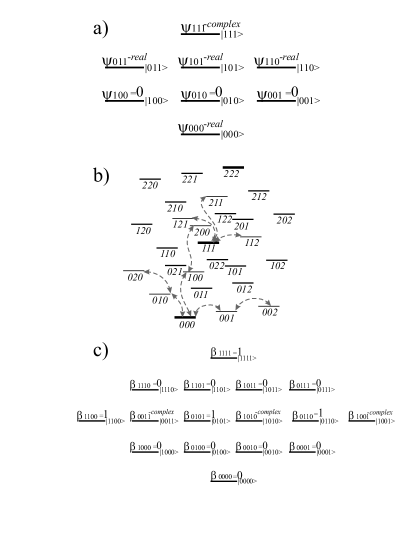
Figure 1: a) Canonic form of the entangled state for three qubits. By a local transformation the amplitudes of the lowest excited states and the phases of the second highest exited states are set to zero. The amplitude of the lowest state is taken as the common factor determining the normalization and the global phase. b) In the case of qudits, the group of local transformations is richer, and the canonic form can be chosen such that it corresponds to maximum population of the symmetric states $\left|k,k,k\right\rangle$ where $k=0,\ldots,d-1$. c) The structure of the tanglemeter for a $4$-qubit system in the case of $SL(2,\mathbb{C})$ local transformations. The scaling factors $q_{i}$ can be chosen in many different ways, in particular such that some of the nonzero coefficients equal one.

II.2 Nilpotent polynomials for entanglement characterization

The amplitudes $\psi$ or $\alpha$ are not the most convenient quantities for characterizing entanglement, since they do not give an immediate idea about the entanglement structure. For instance, for two unentangled qubit pairs, each of which is in a Bell state, one finds

$$\left|\Psi\right\rangle =\frac{1}{2}\left(\left|0,0\right\rangle+\left|1,1\right\rangle\right)\otimes\left(\left|0,0\right\rangle+\left|1,1\right\rangle\right)$$

$$=\psi_{0000}\left|0,0,0,0\right\rangle+\psi_{1100}\left|1,1,0,0\right\rangle$$

$$+\psi_{0011}\left|0,0,1,1\right\rangle+\psi_{1111}\left|1,1,1,1\right\rangle,$$ (11)

where

$$\psi_{0000} =\psi_{1100}=\psi_{0011}=\psi_{1111}=1/2\ ,$$ (12)

$$\alpha_{1100} =\alpha_{0011}=\alpha_{1111}=1\>.$$

In other words, though the system consists of two unentangled parts, each of which is characterized by only one parameter, three non-zero amplitudes $\alpha$ are present in the state vector. This is not convenient and a better description of the entanglement is desirable.

We now introduce a technique which serves this purpose. Consider a standard raising operator

$$\sigma_{i}^{+}=\left(\begin{array}[c]{cc}0&1\\ 0&0\end{array}\right)\,,$$

acting in the $2$-dimensional Hilbert space of the $i$-th qubit. Operators $\sigma_{i}^{+}$ acting on different qubits commute. Since $\left(\sigma_{i}^{+}\right)^{2}=0$, these operators are nilpotent and they can be considered as nilpotent variables. Any quantum state $\left|\Psi\right\rangle$ as in Eq. (1) may be written in the form

$$\left|\Psi\right\rangle =(\psi_{00\ldots 0}+\psi_{00\ldots 1}\sigma_{1}^{+}+\ldots+\psi_{01\ldots 0}\sigma_{n-1}^{+}+\psi_{10\ldots 0}\sigma_{n}^{+}$$

$$+\psi_{00\ldots 11}\sigma_{2}^{+}\sigma_{1}^{+}\ldots+\psi_{11\ldots 0}\sigma_{n}^{+}\sigma_{n-1}^{+}+\ldots)\left|\mathrm{O}\right\rangle$$

$$=\sum_{\{k_{i}\}={0,1}}\psi_{k_{n}k_{n-1}\ldots k_{1}}\prod_{i=1}^{n}\left(\sigma_{i}^{+}\right)^{k_{i}}\left|\mathrm{O}\right\rangle,$$ (13)

where each nilpotent monomial $\prod_{i=1}^{n}\left(\sigma_{i}^{+}\right)^{k_{i}}$ creates the basis state $\left|k_{n},\ldots,k_{1}\right\rangle$ out of the vacuum state $\left|\mathrm{O}\right\rangle$. Let $F(\{\sigma_{i}^{+}\})$ be the nilpotent polynomial

$$F(\{\sigma_{i}^{+}\}) =\sum_{\left\{k_{i}\right\}={0,1}}\alpha_{k_{n}k_{n-1}\ldots k_{1}}\prod_{i=1}^{n}\left(\sigma_{i}^{+}\right)^{k_{i}}$$

$$=\sum_{\{k_{i}\}={0,1}}\frac{\psi_{k_{n}k_{n-1}\ldots k_{1}}}{\psi_{00\ldots 0}}\prod_{i=1}^{n}\left(\sigma_{i}^{+}\right)^{k_{i}}\$$ (14)

containing only the zeroth and first powers of each variable $\sigma_{i}^{+}$. A generic state $\left|\Psi\right\rangle$ normalized to unit vacuum amplitude $\psi_{0\ldots 0}=1$ can thus be written as $F(\{\sigma_{i}^{+}\})|\mathrm{O}\rangle$, with $F(\{\sigma_{i}^{+}\})=1+\alpha_{00\ldots 1}\sigma_{1}^{+}+\ldots$.

Next, define the nilpotential $f(\{\sigma_{i}^{+}\})$ given by the logarithm of $F(\{\sigma_{i}^{+}\})$,

$$f(\{\sigma_{i}^{+}\}) =\ln\left[F(\{\sigma_{i}^{+}\})\right]$$ (15)

$$=\sum_{\{k_{i}\}={0,1}}\beta_{k_{n}k_{n-1}\ldots k_{1}}\prod_{i=1}^{n}\left(\sigma_{i}^{+}\right)^{k_{i}}\ .$$

The coefficients $\beta_{k_{n}k_{n-1}\ldots k_{1}}$ and $\alpha_{k_{n}k_{n-1}\ldots k_{1}}$ can be explicitly related to each other by expanding $\ln F$ in a Taylor series around $1$. This calculation requires at most $n$ operations consisting of multiplications of the polynomial $F-1$, which may generate an exponentially large ($\sim 2^{n}$) number of terms. Note that $\beta_{00\ldots 0}=0$ since $\alpha_{00\ldots 0}=1$, so the nilpotential $f$ starts with the first-order terms. Both $F$ and $f$ contain a finite number of nilpotent terms, at most $2^{n}-1$, with the maximum-order term proportional to the monomial $\prod_{i=1}^{n}\sigma_{i}^{+}$ given by the product of all the nilpotent variables. The canonic form of the state vector corresponds to a polynomial $F_{c}$,

$$F_{c}=1+\alpha_{ij}\sigma_{i}^{+}\sigma_{j}^{+}\ldots\,,$$ (16)

which contains no linear monomials. The corresponding tanglemeter $f_{c}$, also contains no linear terms and reads

$$f_{c}(\{\sigma_{i}^{+}\})=\beta_{ij}\sigma_{i}^{+}\sigma_{j}^{+}+\ldots,\;\;\;$$ (17)

with $\beta_{ij}=\alpha_{ij}$.

The discussion in Sect. II.1 about the canonic form of the state vector applies to the tanglemeter as well. For most purposes, it suffices to employ the form which is unique up to phase changes of the nilpotent variables given by the local transformations $\sigma_{i}^{+}\mapsto\sigma_{i}^{+}\mathrm{e}^{2\mathrm{i}\phi_{i}}$. The coefficients $\beta$ therefore remain invariant up to $n$ phase factors, unless these factors are specified by additional requirements. The phases $\phi_{i}$ may be chosen such that $n$ of non-zero coefficients $\beta$ are set real and positive. Should the tanglemeter of the generic state be defined unambiguously, we can require this for the coefficients $\beta_{k_{n}\ldots k_{1}}$ with $\sum_{i}k_{i}=n-1$, in the same way as it was done for $F$. In special cases, where one or several such coefficients equal zero, some other conditions on the phases may be imposed.

The tanglemeter $f_{c}(\{\sigma_{i}^{+}\})$ immediately allows one to check whether two groups $A$ and $B$ of qubits are entangled or not. The following criterion holds:

The entanglement criterion: The parts $A$ and $B$ of a binary partition of an assembly of $n$ qubits are unentangled iff

$$\frac{\partial^{2}f_{c}(\{x_{i}\})}{\partial x_{k}\partial x_{m}}=0\,,\;\;\;\forall k\in A,\>\forall m\in B\>.$$ (18)

In other words, the subsystems $A$ and$~{}B$ of the partition are disentangled iff $f_{A\cup B}=f_{A}(\left\{x_{\in A}\right\})+f_{B}(\left\{x_{\in B}\right\})$, and no cross terms are present in the tanglemeter. Note that the criterion of Eq. (18) holds not only for the tanglemeter $f_{c}$, but for the nilpotential $f$ as well. However, we formulate the criterion in terms of $f_{c}$, because the coefficients $\beta$ of the tanglemeter are uniquely defined by construction.

II.3 Examples: Canonic forms for two, three, and four qubits

For two qubits the result is immediate

$$f_{c}=\beta_{11}\sigma_{2}^{+}\sigma_{2}^{+},\qquad F_{c}=1+\alpha_{11}\sigma_{2}^{+}\sigma_{2}^{+}=1+\beta_{11}\sigma_{2}^{+}\sigma_{1}^{+}\,,$$ (19)

where the constant $\alpha_{11}=\beta_{11}$ can be chosen real. For three qubits, the canonic forms of $F$ and $f$ also differ only by the unity term,

$$f_{c}=\beta_{3}\sigma_{2}^{+}\sigma_{1}^{+}+\beta_{5}\sigma_{3}^{+}\sigma_{1}^{+}+\beta_{6}\sigma_{3}^{+}\sigma_{2}^{+}+\beta_{7}\sigma_{3}^{+}\sigma_{2}^{+}\sigma_{1}^{+}=F_{c}-1\,.$$ (20)

Here, we have introduced a shorter notation by considering the indices of $\beta$ as binary representation of decimal numbers, $011\rightarrow 3$, etc. One can make use of the fact that the variables $\sigma_{i}^{+}$ are defined up to phase factors, and set $\beta_{3}$, $\beta_{5}$, and $\beta_{6}$ real. Expressing the invariants of Eqs. (5)-(6) via the parameters in the canonic form, we obtain

$$I_{1} =1+2|\beta_{7}|^{2}\left(\beta_{3}^{2}+\beta_{5}^{2}+\beta_{6}^{2}\right)+|\beta_{7}|^{4}+2\beta_{3}^{2}+\beta_{3}^{4}+2\beta_{5}^{2}\beta_{6}^{2}\ ,$$

$$\newline I_{2} =1+2|\beta_{7}|^{2}\left(\beta_{3}^{2}+\beta_{5}^{2}+\beta_{6}^{2}\right)+|\beta_{7}|^{4}+2\beta_{5}^{2}+\beta_{5}^{4}+2\beta_{3}^{2}\beta_{6}^{2}\ ,$$

$$\newline I_{3} =1+2|\beta_{7}|^{2}\left(\beta_{3}^{2}+\beta_{5}^{2}+\beta_{6}^{2}\right)+|\beta_{7}|^{4}+2\beta_{6}^{2}+\beta_{6}^{4}+2\beta_{3}^{2}\beta_{5}^{2}\ ,$$

$$\newline I_{4}+iI_{5} =2\left(\beta_{7}^{2}+4\beta_{3}\beta_{5}\beta_{6}\right)\ .$$ (21)

This explicitly illustrates their linear independence.

The tanglemeter for four qubits reads

$$f_{c} =\beta_{3}\sigma_{2}^{+}\sigma_{1}^{+}+\beta_{5}\sigma_{3}^{+}\sigma_{1}^{+}+\beta_{9}\sigma_{4}^{+}\sigma_{1}^{+}+\beta_{6}\sigma_{3}^{+}\sigma_{2}^{+}+\beta_{10}\sigma_{4}^{+}\sigma_{2}^{+}+\beta_{12}\sigma_{4}^{+}\sigma_{3}^{+}$$ (22)

$$+\beta_{7}\sigma_{3}^{+}\sigma_{2}^{+}\sigma_{1}^{+}+\beta_{13}\sigma_{4}^{+}\sigma_{3}^{+}\sigma_{1}^{+}+\beta_{11}\sigma_{4}^{+}\sigma_{2}^{+}\sigma_{1}^{+}+\beta_{14}\sigma_{4}^{+}\sigma_{3}^{+}\sigma_{2}^{+}+\beta_{15}\sigma_{4}^{+}\sigma_{3}^{+}\sigma_{2}^{+}\sigma_{1}^{+},$$

while the coefficients $\alpha_{i}$ of the polynomial $F_{c}$ differ from $\beta_{i}$ only at the last position

$$\alpha_{15}=\beta_{15}+\beta_{3}\beta_{12}+\beta_{5}\beta_{10}+\beta_{9}\beta_{6}.$$ (23)

One may note that the sums of the indices of the factors in this expression are equal. The latter is a general feature for the relationship among the coefficients $\alpha$ and $\beta$: the coefficients $\alpha$ are given by sums of terms, each of which contains a product of the coefficients $\beta$ where the sum of the indices equals the index of $\alpha$. We also note that a proper set of invariants of $\otimes_{i=1}^{4}SU_{i}(2)\otimes\mathbb{C}^{*}$ expressed via the components $\psi$ of the state vector can, in principle, be related to the tanglemeter coefficients, in analogy to the relation between Eqs. (5-6) and Eq. (21) for $\otimes_{i=1}^{4}SU_{i}(2)$ invariants.

II.4 Tanglemeter and entanglement classes for $SL(2,\mathbb{C})$ operations

We now take a larger class of local operations and consider arbitrary invertible linear transformations $GL$, instead of just the unitary transformations $SU$. Invertible transformations with non-zero determinant correspond in general to indirect measurements, that are measurements performed over an auxiliary system prepared in a certain fixed quantum state after it has interacted with the system under consideration. Besides allowing the realization of measurements more general than projective Von Neumann measurements QI , this procedure may serve as a tool for quantum control and quantum state engineering Vogel . In the case where a single copy purification of a quantum state is considered, the outcome of the measurements is not achieved with certainty. Therefore, a stochastic factor allowing for the outcome probability should be taken into account, whence the resulting state vector has to be renormalized in accordance. Since the normalization factor in the latter require an information about the initial state vector, they do not strictly speaking form a group. In our approach, we do not impose a normalization condition on the wave function whatsoever and will be interested in finding the invariants Verstraete2 of the transformations belonging to the group $\mathcal{G}=\otimes_{i}SL_{i}(2,\mathbb{C})\otimes\mathbb{C}^{*}$, where $\mathbb{C}^{*}$ describes as before multiplication by an arbitrary nonzero complex number and the transformations $\in SL_{i}(2,\mathbb{C})$ multiply the $i$th qubit state vector by a $2\times 2$ matrix of unit determinant. Another way to represent $\mathcal{G}$ is to express it as the product $\otimes_{i}GL_{i}(2,\mathbb{C})$ and factorize it over $n-1$ redundant factors $\mathbb{C}^{*}$. The factors $\mathbb{C}^{*}$ in each $GL_{i}(2,\mathbb{C})$ describe the same wave function transformations.

We emphasize that the change of the wave function renormalization does not result exclusively from the transformations $\in\mathbb{C}^{*}$, but from some $SL(2,\mathbb{C})$ transformations as well, and in particular, the transformations $\sim\exp{q\sigma_{i}^{z}}$ with complex $q$. Thus, considering just $\otimes_{i}SL_{i}(2,\mathbb{C})$ instead of the full group $\mathcal{G}$ may not have an explicit physical sense. Still, we will do it sometimes to better reveal the mathematical structure of the results obtained. Since the local $SL$ transformations comprise the key part of $\mathcal{G}$, and following the established usus we will mainly refer to them and talk about $sl$-entanglement in assemblies subject to indirect local measurements.

Though local, $SL$ operations can modify the set of quantities which characterizes entanglement in assemblies subject to local $SU$ transformations. Since $SU\subset SL$, many different $su$-orbits become equivalent under local $SL$ transformations. In other words, the orbits of local $SL$ transformations contain the $su$-orbits as subsets. Classification of $sl$-orbits reveals the entanglement which persists despite the indirect measurements. In order to distinguish this type of entanglement from the invariants under local unitary transformations, one may call it $sl$-entanglement. In particular, classification for three-qubit assembly Dur shows that all generic quantum states belong to one orbit of $\mathcal{G}$, which includes the canonic Greenberger-Horne-Zeilinger (GHZ) state $(\left|000\right\rangle+\left|111\right\rangle)/\sqrt{2}$ GHZ . The invariant Eq. (6) also known as $3$-tangle $\tau$ Wootters , is different from zero only for this general orbit, and the value of $\tau$ calculated for the state amplitudes normalized to unit probability descriminates different $su$-orbits within this single general $sl$-orbit. The states with $\tau=1$ can be reduced to GHZ state by local unitary transformations, while for other states, with $\tau<1$ indirect local measurements are required for the purpose. Moreover, there are five singular orbits of $\mathcal{G}$ with $\tau=0$ that contain the states irreducible to GHZ-state. For four-qubit assemblies, the classification Verstraete becomes much more involved, but still it gives an idea about the types of entanglement and eventual measures.

Each element of the $SL_{i}(2,\mathbb{C})$ group, that is isomorphic to the Lorentz group $SO(3,1)$, involves 6 parameters. In the general case, the number of invariants,

$$D_{sl}\ =\ 2^{n+1}-6n-2$$ (24)

is less than that for unitary transformations Eq.( 3). This counting is valid and returns a positive value for $n\geq 4$ when the actions of different local operations are linearly independent. For $n=2,~{}3$ where the number of the parameters in the group is more than the number of the parameters in the wave function, and the result of some local $SL$ are redundant, no invariants exist. In particular, for two qubits, any generic state is equivalent under $\mathcal{G}$ to the Bell state and for 3 qubits — to the GHZ state. For four qubits, there are $6$ real invariants, for $n=5$, $D_{sl}=32$, etc.

A smaller number of $sl$-invariants Eq. (24) as compared to that of $su$-invariants Eq. (3) implies that different $su$-orbits may belong to the same $sl$-orbit. In analogy to the $su$-canonic state, one has to define a $sl$-canonic state as the marker of a $sl$-orbit. In contrast to the unitary case where the canonic state has been defined by the condition of maximum reference state population, for $SL$ transformations we introduce directly canonic form of the tanglemeter. To this end, we impose the following conditions: in addition to the requirement of the Eq. (9), i.e. all $n$ linear in $\sigma^{+}$ terms of the nilpotential equal to zero, we require that all $n$ terms of $(n-1)$-th order vanish as well. In other words, the $sl$-tanglemeter takes the form

$$f_{C}(\{\sigma_{i}^{+}\})=\sum_{\quad\Sigma_{i}k_{i}\neq\{1,n-1\}}\beta_{k_{n}k_{n-1}\ldots k_{1}}\prod_{i=1}^{n}\left(\sigma_{i}^{+}\right)^{k_{i}},$$ (25)

and in this way we have specified $4n$ out of the $6n$ real parameters of the local transformations that bring a given state to the $sl$-canonic form. We thus left with $2n$ parameters that have to be specified.

In contrast to the unitary case, where the nilpotent variables $\sigma^{+}$ are defined up to arbitrary phase factors, for $SL$ transformations the variables in Eq. (25) are defined up to a complex-valued scaling factor $\sigma_{i}^{+}\mapsto\sigma_{i}^{+}q_{i}$. One can further specify the $sl$-tanglemeter by choosing these factors such that $n$ complex coefficients of the tanglemeter are set to unity. If convenient, one can impose another set of $n$ requirements.

As a first example, consider the three-qubit case. The $sl$-tanglemeter Eq. (25) for a generic three-qubit state reads

$$f_{C}=\sigma_{3}^{+}\sigma_{2}^{+}\sigma_{1}^{+},$$ (26)

where the coefficient is set to unity by the scale freedom in the definition of the nilpotent variables. The corresponding wave function $F_{C}$ is nothing but the GHZ state. This shows again that all generic states belong to the same $sl$-orbit, which includes this state. There are, however, also three distinct singular classes of entangled states of measure zero Dur whose tanglemeters do not involve the product $\sigma_{1}^{+}\sigma_{2}^{+}\sigma_{3}^{+}$ and have one of the following forms,

$$f_{C}=\sigma_{2}^{+}\sigma_{1}^{+}+\sigma_{3}^{+}\sigma_{1}^{+}\>,$$

$$f_{C}=\sigma_{3}^{+}\sigma_{1}^{+}+\sigma_{3}^{+}\sigma_{2}^{+}\>,$$

$$f_{C}=\sigma_{2}^{+}\sigma_{1}^{+}+\sigma_{3}^{+}\sigma_{2}^{+}\>.$$

In this classification, we have only taken into account the states whose tanglemeters involve all three $\sigma_{i}^{+}$ such that no qubit is completely disentangled from the others.

For a generic four-qubit state one finds the $sl$-tanglemeter

$$f_{C} =\beta_{3}\sigma_{2}^{+}\sigma_{1}^{+}+\beta_{5}\sigma_{3}^{+}\sigma_{1}^{+}+\beta_{9}\sigma_{4}^{+}\sigma_{1}^{+}+\beta_{6}\sigma_{3}^{+}\sigma_{2}^{+}$$ (27)

$$+\beta_{10}\sigma_{4}^{+}\sigma_{2}^{+}+\beta_{12}\sigma_{4}^{+}\sigma_{3}^{+}+\beta_{15}\sigma_{4}^{+}\sigma_{3}^{+}\sigma_{2}^{+}\sigma_{1}^{+}\,,$$

where the scaling factors $q_{i}$ of the variables $\sigma_{i}^{+}$ can be specified such that this form becomes equivalent to the expression given in Theorem 2 of Ref. Verstraete :

$$f_{C} =\beta_{3}\left(\sigma_{1}^{+}\sigma_{2}^{+}+\sigma_{3}^{+}\sigma_{4}^{+}\right)+\beta_{5}\left(\sigma_{1}^{+}\sigma_{3}^{+}+\sigma_{2}^{+}\sigma_{4}^{+}\right)$$ (28)

$$+\beta_{6}\left(\sigma_{1}^{+}\sigma_{4}^{+}+\sigma_{2}^{+}\sigma_{3}^{+}\right)+\sigma_{1}^{+}\sigma_{2}^{+}\sigma_{3}^{+}\sigma_{4}^{+}.$$

In Fig. 1 c), we illustrate the structure of $sl$-tanglemeter for this case with an alternative choice of the scaling factors.

It is worth mentioning that, though any generic nilpotential can be reduced to the canonic form of Eq. (25) this turns out to be impossible for some sets of states of measure zero, as it is already the case for three qubits. These sets may play an important role for applications and can be grouped into special classes. Some of these classes are shown in Sect. III.4.3 at the example of four qubits. There we also present an explicit algorithm for evaluation of $sl$-tanglemeters based on the stationary solutions of dynamic equations with feedbacks imposed on the parameters of local transformations. This yields the special entanglement classes in a natural way as singular stationary solutions.

We conclude this section by discussing the precise mathematical meaning of the canonic states. The renormalization of the wave function that follows the maximization of the reference state amplitudes by local $SU$ transformations belongs to the group $\mathbb{C}^{*}$ of multiplication by a complex number $\kappa$. Therefore, strictly speaking, the applied transformations belong to the group $\otimes_{i}SU_{i}(2)\otimes\mathbb{C}^{*}$. However, the group $\otimes_{i}SU_{i}(2)$ does not affect the normalization of the state vector, while the requirement $\psi_{{\rm O}}=1$ imposed on the canonic state uniquely specifies the number $\kappa$ thus allowing to introduce the tanglemeter as a characteristic of $sl$-orbits. In other words, once the condition $\psi_{{\rm O}}=1$ is satisfied, the group $\otimes_{i}SU_{i}(2)\otimes\mathbb{C}^{*}$ becomes isomorphic to the group $\otimes_{i}SU_{i}(2)$.

This is no longer the case for indirect measurements. Neither the group $G$ nor its nontrivial part $\otimes_{i}SL_{i}(2,\mathbb{C})$ conserve the state normalization. By imposing the requirement $\psi_{{\rm O}}=1$, we mark an orbit of $G/\mathbb{C}^{*}$, and thereby specify the structure of the canonic state given by the state amplitude ratios $\psi_{i}/\psi_{{\rm O}}$ expressed in terms of the $sl$-tanglemeter coefficients. However, a state of same structure but with a different normalization can be physically achieved in many different ways, – as a result of a single indirect measurement, or a sequence of two or more indirect measurements. The probability to obtain an outcome of the measurements that correspond to required $G/\mathbb{C}^{*}$ transformation thus depends on the particular choice of the measurement procedure. Therefore, the complex factor $\kappa$ can be an arbitrary number, irrelevent to the values of the $sl$-tanglemeter coefficients.

However, when we consider just the nontrivial part $\otimes_{i}SL_{i}(2,\mathbb{C})$ of $G$, the factor $\kappa$ can bear certain physical significance. In fact, a transformation from $\otimes_{i}SL_{i}(2,\mathbb{C})$ may bring a state initially normalized to unit probability to another one, which differs from the canonic state only by a factor $\kappa$. In this case the factor $\kappa$ is uniquely defined function of the initial state xx . When the transformation is unitary $\kappa$ amounts to $1/\sqrt{\sum_{i}\left|\psi_{i}\right|^{2}}$ where the amplitudes $\psi_{i}$ of the canonic state are normalized to unity reference state amplitude, as required. For non-unitary $SL$ transformations this quantity is different. Therefore, $ln\left(\left|\kappa\sqrt{\sum_{i}\left|\psi_{i}\right|^{2}}\right|\right)$ can serve as a measure of non-unitarity of the transformation that discriminates different $su$-orbits that belong to the same $G$-orbit.

II.5 How do the nilpotent polynomials relate to existing entanglement measures

In general, there is no universal and precise definition of proper measures of entanglement MLV , with the exception of bipartite entanglement: as long as we are interested in entanglement between two parts $A$ and $B$ of a quantum system in a pure state, natural measures of such entanglement do exist. They are based on the reduced density operator $\rho_{A}$ of either part, obtained by tracing over the quantum numbers corresponding to the other part $B$. In particular, $S_{vN}=-\mathrm{Tr}[\rho_{A}\log\rho_{A}]$ and $S_{l}=1-\mathrm{Tr}[\rho_{A}^{2}]$, give the von Neumann and the linear entropies, respectively QI , as already mentioned in the Introduction. Clearly, both characteristics can be directly related to the tanglemeter parameters. However, the explicit formulae giving these relations, which are simple for the case of two qubits

$$S_{l} =\frac{2\left|\beta_{11}\right|^{2}}{\left(1+\left|\beta_{11}\right|^{2}\right)^{2}},$$

$$S_{vN} =\ln\left[1+\left|\beta_{11}\right|^{2}\right]-\frac{\left|\beta_{11}\right|^{2}}{1+\left|\beta_{11}\right|^{2}}\ln\left[\left|\beta_{11}\right|^{2}\right]~{},$$

become awkward for larger numbers of qubits within the bipartition, as well as for higher-dimensional elements. This reflects the fact that the coefficients of nilpotent polynomials carry much more information about entanglement than the simple bipartite correlations captured by the entropy measures.

Another useful entanglement measure, concurrence $C$, has been introduced in Ref. Wootters in the context of mixed two-qubit states, and has been employed for constructing the residual entanglement $\tau$, as a measure characterizing three-qubit pure-state entanglement and possibly beyond Wong ; Akhtarshenas . Both $C$ and $\tau$ may be expressed in terms of the amplitudes $\psi$ of the $su$-canonic state and in terms of the tanglemeter coefficients $\beta$ Eq. (20). The concurrence between the first and the second qubits reads

$$C_{12} =2\Big{|}|\psi_{000}\psi_{110}|-|\psi_{101}\psi_{011}|\Big{|}$$

$$=\frac{2||\beta_{6}|-|\beta_{5}\beta_{3}||}{1+\beta_{6}^{2}+\beta_{5}^{2}+\beta_{3}^{2}+|\beta_{7}|^{2}}~{}.$$ (29)

The residual entanglement, or $3$-tangle, has the form of a fourth-order polynomial in the amplitudes. For the canonic state, it reads

$$\tau_{3} =4\Big{|}\left(\psi_{000}\psi_{111}\right)^{2}+4\psi_{000}\psi_{110}\psi_{101}\psi_{011}\Big{|}$$

$$=\frac{4\left|\beta_{7}{}^{2}+4\beta_{6}\beta_{5}\beta_{3}\right|}{\left(1+\beta_{6}^{2}+\beta_{5}^{2}+\beta_{3}^{2}+|\beta_{7}^{2}|\right)^{2}}\,,$$ (30)

which up to a numerical factor is equal to the invariant $\left|I_{4}+iI_{5}\right|$ of Eqs. (6, 21) divided by the normalization factor $\sum|\psi|^{2}=1+\beta_{6}^{2}+\beta_{5}^{2}+\beta_{3}^{2}+|\beta_{7}^{2}|$. The presence of the normalization factor in the denominators of Eqs. (29), (30) is due to the fact that these quantities are usually calculated for the state vector normalized to unity while the coefficients $\beta$ refer to the tanglemeter that is the logarithm of the canonical wave function with the normalization $\psi_{000}=1$.

What are convenient measures that can be introduced to characterize $sl$–entanglement? We have seen that all generic states of the assembly of three qubits belong to the same orbit of $\mathcal{G}$ and strictly speaking there are no invariant measures at all. However, the $su$-invariant $I_{4}+iI_{5}$ of Eq. (6) remains invariant under the restricted class of transformations $\otimes_{i=1}^{3}SL_{i}(2,\mathbb{C})$, while the other $SU$ invariants $I_{1,2,3}$ of Eq. (5) depending on  both $\psi$ and $\psi^{\ast}$ change under $SL$ transformations. Hence, in this restricted sense it may serve as a measure for $sl$-entanglement.

The measures characterizing the $sl$-entanglement for a 4-qubit assembly can be constructed in a similar way. We take products of several factors $\sim\psi$ (but not the factors $\sim\psi^{\ast}$) and convolute it over $SU(2)$ indices with invariant tensors $\epsilon^{ii^{\prime}}$ footnote0 . The simplest combination

$$I^{(2)}\ =\ \psi_{ijkl}\psi^{ijkl}\,$$ (31)

is $sl$-invariant and can be taken as a characteristic of $sl$-entanglement, remaining not invariant only with respect to the transformations $\in\mathbb{C}^{\ast}$. There are three different $sl$-invariants $\sim\psi^{4}$,

$$I_{12}^{(4)} =I_{34}^{(4)}\ =\ \psi_{ijkl}\psi^{ijmn}\psi_{opmn}\psi^{opkl}\,,$$

$$I_{13}^{(4)} =I_{24}^{(4)}\ =\ \psi_{ikjl}\psi^{imjn}\psi_{ompn}\psi^{okpl}\,,$$

$$I_{14}^{(4)} =I_{23}^{(4)}\ =\ \psi_{iklj}\psi^{imnj}\psi_{omnp}\psi^{oklp}\,.$$ (32)

The ratios $I_{12}^{(4)}/(I^{(2)})^{2}$, $I_{13}^{(4)}/(I^{(2)})^{2}$, and $I_{14}^{(4)}/(I^{(2)})^{2}$ are in addition invariant with respect to multiplication of the state vector by an arbitrary complex constant and thereby they are invariants of $\mathcal{G}$. Were these ratio linearly independent, they would give us a complete characterization of $4$-qubit entanglement, since the $4$-qubit $sl$-tanglemeter Eq. (28) involves $3$ complex parameters. However, they are not. The following identity

$$I_{12}^{(4)}+I_{13}^{(4)}+I_{14}^{(4)}\ =\ \frac{3}{2}\left(I^{(2)}\right)^{2}\,$$ (33)

makes these quantities inconvenient for the entanglement characterization.

We therefore turn to the $6$-th order invariants and consider following three functionally independent combinations

$$I_{12}^{(6)}\ =\frac{1}{6}\ \left(\psi_{ingd}\psi_{mrko}\psi_{sjph}-\psi_{ingo}\psi_{mrkh}\psi_{sjpd}\right)\psi^{mrgd}\psi^{inph}\psi^{sjko}\,,$$

$$I_{23}^{(6)}\ =\frac{1}{6}\ \left(\psi_{ijpo}\psi_{mngh}\psi_{srkd}-\psi_{ijpd}\psi_{mngo}\psi_{srkh}\right)\psi^{mrgd}\psi^{inph}\psi^{sjko}\,,$$

$$I_{13}^{(6)}\ =\frac{1}{6}\ \left(\psi_{ijkh}\psi_{mnpd}\psi_{srgo}-\psi_{ijgh}\psi_{mnkd}\psi_{srpo}\right)\psi^{mrgd}\psi^{inph}\psi^{sjko}\,,$$ (34)

whose differences give the invariants Eq. (32) multiplied by $I^{(2)}$. Explicit form of these invariants for a generic state is awkward. However they take a simple form

$$I^{(2)} =\psi_{0000}^{2}(t+x+y+z)$$

$$I_{12}^{(6)}\ =4\ \psi_{0000}^{6}\left(t+x-y-z\right)(tx-yz)\,,$$

$$I_{23}^{(6)}\ =4\ \psi_{0000}^{6}\left(t-x+y-z\right)(ty-xz)\,,$$

$$I_{13}^{(6)}\ =4\ \psi_{0000}^{6}\left(t-x-y+z\right)(tz-xy)\,,$$ (35)

for the canonic state, where the $sl$-tanglemeter Eq. (28) suggests

$$\psi_{1100} = \psi_{0011}=\psi_{0000}\sqrt{x}$$

$$\psi_{1001} = \psi_{1001}=\psi_{0000}\sqrt{y}$$

$$\psi_{0101} = \psi_{1010}=\psi_{0000}\sqrt{z}$$

$$\psi_{1111} = \psi_{0000}t$$

for the nonvanishing amplitudes, and where the notations $x=\beta_{3}^{2}$, $y=\beta_{5}^{2}$, $z=\beta_{6}^{2}$, and $t=\psi_{1111}=1+x+y+z$ are employed. We introduce new variables

$$X\ =\psi_{0000}^{2}\left(t+x-y-z\right),$$

$$Y\ =\ \psi_{0000}^{2}\left(t-x+y-z\right)\,,$$

$$Z\ =\psi_{0000}^{2}\left(t-x-y+z\right)\,,$$ (36)

and find

$$I_{12}^{(6)}\ =X(I^{(2)}X-YZ)\,,$$

$$I_{23}^{(6)}\ =Y(I^{(2)}Y-XZ)\,,$$

$$I_{13}^{(6)}\ =Z(I^{(2)}Z-XY)\,.$$

Solving this system of equations yields

$$X =\sqrt{(I_{12}^{(6)}+P)/I^{(2)}}\ \,,$$

$$\ Y =\sqrt{(I_{23}^{(6)}+P)/I^{(2)}}\,,$$

$$\ Z =\sqrt{(I_{13}^{(6)}+P)/I^{(2)}}\,,$$ (37)

where $P$ is a root  of a cubic equation

$$(I_{13}^{(6)}+P)(I_{23}^{(6)}+P)(I_{12}^{(6)}+P)=\left(I^{(2)}\right)^{2}P^{2}.$$

Different roots of these equations and different signs of the square roots in Eq. (37) yield different $sl$-canonic states, that either coincide or are related by $SL$ transformations. The amplitudes of these states can be written explicitly

$$\psi_{0000} = \frac{\sqrt{\sqrt{I_{13}^{(6)}+P}+\sqrt{I_{23}^{(6)}+P}+\sqrt{I_{12}^{(6)}+P}-\left(I^{(2)}\right)^{3/2}}}{\sqrt{2}\left(I^{(2)}\right)^{1/4}},$$

$$\psi_{1100} = \psi_{0011}=\frac{\sqrt{\sqrt{I_{13}^{(6)}+P}-\sqrt{I_{23}^{(6)}+P}-\sqrt{I_{12}^{(6)}+P}+\left(I^{(2)}\right)^{3/2}}}{2\left(I^{(2)}\right)^{1/4}},$$

$$\psi_{1001} = \psi_{1001}=\frac{\sqrt{\sqrt{I_{23}^{(6)}+P}-\sqrt{I_{13}^{(6)}+P}-\sqrt{I_{12}^{(6)}+P}+\left(I^{(2)}\right)^{3/2}}}{2\left(I^{(2)}\right)^{1/4}},$$

$$\psi_{0101} = \psi_{1010}=\frac{\sqrt{\sqrt{I_{12}^{(6)}+P}-\sqrt{I_{23}^{(6)}+P}-\sqrt{I_{13}^{(6)}+P}+\left(I^{(2)}\right)^{3/2}}}{2\left(I^{(2)}\right)^{1/4}},$$

$$\psi_{1111} = \frac{\sqrt{I_{13}^{(6)}+P}+\sqrt{I_{23}^{(6)}+P}+\sqrt{I_{12}^{(6)}+P}+\left(I^{(2)}\right)^{3/2}}{2\sqrt{2}\left(I^{(2)}\right)^{1/4}\sqrt{\sqrt{I_{13}^{(6)}+P}+\sqrt{I_{23}^{(6)}+P}+\sqrt{I_{12}^{(6)}+P}-\left(I^{(2)}\right)^{3/2}}},$$ (38)

while the ratios $\psi_{1100}/\psi_{0000}$, $\psi_{1001}/\psi_{0000}$, and $\psi_{0101}/\psi_{0000}$ yield the $sl$-tanglemeter coefficients $\beta_{3}$, $\beta_{5}$, and $\beta_{6}$, respectively. Thus, the $sl$-entanglement in the $4$-qubit assembly can be completely characterized by three independent scale–invariant complex ratios

$$\beta_{3} = \frac{\sqrt{\sqrt{I_{13}^{(6)}+P}-\sqrt{I_{23}^{(6)}+P}-\sqrt{I_{12}^{(6)}+P}+\left(I^{(2)}\right)^{3/2}}}{\sqrt{2}\sqrt{\sqrt{I_{13}^{(6)}+P}+\sqrt{I_{23}^{(6)}+P}+\sqrt{I_{12}^{(6)}+P}-\left(I^{(2)}\right)^{3/2}}},$$

$$\beta_{5} = \frac{\sqrt{\sqrt{I_{23}^{(6)}+P}-\sqrt{I_{13}^{(6)}+P}-\sqrt{I_{12}^{(6)}+P}+\left(I^{(2)}\right)^{3/2}}}{\sqrt{2}\sqrt{\sqrt{I_{13}^{(6)}+P}+\sqrt{I_{23}^{(6)}+P}+\sqrt{I_{12}^{(6)}+P}-\left(I^{(2)}\right)^{3/2}}},$$

$$\beta_{6} = \frac{\sqrt{\sqrt{I_{12}^{(6)}+P}-\sqrt{I_{23}^{(6)}+P}-\sqrt{I_{13}^{(6)}+P}+\left(I^{(2)}\right)^{3/2}}}{\sqrt{2}\sqrt{\sqrt{I_{13}^{(6)}+P}+\sqrt{I_{23}^{(6)}+P}+\sqrt{I_{12}^{(6)}+P}-\left(I^{(2)}\right)^{3/2}}},$$

coming from the invariants Eqs. (34,31).

As for a measure characterizing entanglement for $4$ qubits, one has to consider at least two quantities. The first is the sum $\sum\left|\psi^{2}\right|$ over the amplitudes Eq. (38), which gives the regular normalization of the canonic-like state. Once the invariants of Eqs. (31), (34) are calculated for a state normalized to $1$, this sum shows how the $SL$ transformation required for setting the state to the canonic form is different from a unitary transformation, whence $\left|\ln\sum\left|\psi^{2}\right|\right|$ provides us with a measure of this nonunitary. The root $P$ and the signs of the square roots Eq. (37) have to be chosen such that $\left|\ln\sum\left|\psi^{2}\right|\right|$ is minimum. This quantity discriminates different $su$-orbits that belong to the same $sl$-orbit in analogy to the $3$-tangle, which discriminates different $su$-orbits within a single generic $SL$ orbit of $3$-qubit assembly. It may serve as a measure of $su$-entanglement within a $sl$-orbit. The second quantity has to discriminate different $sl$-orbits and serve as a measure of $sl$-entanglement. A natural candidate for that is the sum of moduli squared of the $sl$-tanglemeter coefficients $\beta$, which takes value $0$ for $GHZ$ canonic state, remaining larger for all other states. The choice of $P$ and the signs in Eq. (37) has to be done such that this quantity is minimum. This measure shows us how close is the orbit to the $GHZ$ orbit.

One may also ask for simpler measures that would be polynomials on the state amplitudes $\psi$. It turns out that two such characteristics, $\left|I^{(2)}\right|$ and $\left(\left|I_{13}^{(6)}\right|+\left|I_{23}^{(6)}\right|+\left|I_{12}^{(6)}\right|\right)/$ $\left|I^{(2)}\right|^{2}$, can be directly associated with the $su$ and $sl$-measures. In Fig. 2 we show these characteristics plotted versus $\exp\left|\ln\sum\left|\psi^{2}\right|\right|$ and $\sum\left|\beta^{2}\right|$, respectively, for a variety of $\sim 10^{2}$ randomly chosen assembly states normalized to unity. One sees that $\left|I^{(2)}\right|$ strongly correlates with the measure of non-unitarity, while the sum of the moduli of $6$-th order invariants majorates the $sl$-entanglement measure based on the $sl$-tanglemeter coefficients. Other combinations of invariants do not correlate with the tanglemeter coefficients.

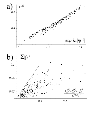
Figure 2: a) The polynomial invariant $\left|I^{(2)}\right|$ plotted versus the non-unitarity measure $\exp\left|\ln\sum\left|\psi^{2}\right|\right|$ for a set of $\sim 10^{2}$ randomly chosen assembly states. b) Same for the combination $\left(\left|I_{13}^{(6)}\right|+\left|I_{23}^{(6)}\right|+\left|I_{12}^{(6)}\right|\right)/$ $\left|I^{(2)}\right|^{2}$ and the $\sum\left|\beta^{2}\right|$given by the $sl$-tanglemeter.

III Quantum state operations and dynamics in terms of the nilpotent polynomials

In this section, we first describe the effects of local and gate transformations on the assembly state vector as algebraic manipulations of the corresponding polynomials $F$ and $f$. In principle, by applying a properly chosen sequence of finite local transformations, one can reduce a nilpotent polynomial to the canonic form, thereby specifying the tanglemeter. However, straightforwardly applying these transformations is not a very practical way to proceed, since it usually requires lengthy calculations.

We therefore turn to infinitesimal transformations second, and derive the equations of motion describing the dynamics of the nilpotential under continuous local and gate operations. We show that, for an important class of Hamiltonians supporting universal quantum computation, the dynamic equation for the nilpotential acquires a well-known Hamilton-Jacobi form.

We thirdly demonstrate how to determine the tanglemeter with the help of such equation. To this end, a proper feedback is required, ensuring that the parameters of infinitesimal $SU(2)$ or $SL(2,\mathbb{C})$ transformations are adjusted to track current values of the nilpotential coefficients. The tanglemeter appears as a stable stationary solution, that is a focus of the resulting equation. We illustrate this method in the example of four qubits. We show how to find the $sl$-tanglemeter for a generic $4$-qubit state and how to explicitly identify a number of special classes that cannot be reduced to this form. For these classes we suggest alternative natural tanglemeters.

III.1 Local operations

A general local unitary transformation Eq. (2) applied to $i$-th qubit can also be expressed in the equivalent form

$$U_{i}=\mathrm{e}^{A_{i}\sigma_{i}^{-}}\mathrm{e}^{B_{i}\sigma_{i}^{z}}\mathrm{e}^{C_{i}\sigma_{i}^{+}},~{}~{}$$ (39)

which better suits the consideration in terms of nilpotential polynomials, since each step of the local transformation can be expressed as an operation linear in $\sigma$, that is

$$\mathrm{e}^{C_{i}\sigma_{i}^{+}} =1+C_{i}\sigma_{i}^{+}\,,$$

$$\mathrm{e}^{B_{i}\sigma_{i}^{z}} =\mathrm{cos}\left(B_{i}\right)+\mathrm{sin}\left(B_{i}\right)\sigma_{i}^{z}\,,$$

$$\mathrm{e}^{A_{i}\sigma_{i}^{-}} =1+A_{i}\sigma_{i}^{-}\,.$$

The explicit expressions

$$A_{i} =\frac{\left(\mathrm{i}P_{i}^{x}-P_{i}^{y}\right)\sin P}{P\cos P+\mathrm{i}P_{i}^{z}\sin P};\ B_{i}=\log\left[\cos P+\frac{\mathrm{i}P_{i}^{z}\sin P}{P}\right];$$

$$C_{i} =\frac{\left(\mathrm{i}P_{i}^{x}+P_{i}^{y}\right)\sin P}{P\cos P+\mathrm{i}P_{i}^{z}\sin P};\ P=\sqrt{{\textstyle\sum\limits_{\kappa=x,y,z}}\left(P_{i}^{\kappa}\right)^{2}}$$ (40)

relate the parameters in Eq. (2) and Eq. (39).

The transformations Eq. (39) act on the state vector $|\Psi\rangle=F(\{\sigma_{i}^{+}\})|\mathrm{O}\rangle$ and yield a transformed state $F^{\prime}(\{\sigma_{i}^{+}\})|\mathrm{O}\rangle$. One can formalize the rules allowing one to obtain $F^{\prime}$ from $F$. Bearing in mind that $\sigma^{-}|0\rangle=0$ and $\sigma^{z}|0\rangle=-|0\rangle$, one can represent the action of $\sigma_{i}^{+},\sigma_{i}^{z},\sigma_{i}^{-}$ as appropriate differential operations for the nilpotent variable $\sigma^{+}_{i}$. The application of the operator $\sigma_{i}^{+}$ is straightforward – it is a direct multiplication: this operation eliminates the terms that were proportional to $\sigma_{i}^{+}$ prior to the multiplication. The application of $\sigma_{i}^{-}$ is a kind of inverse: it can be considered as a derivative with respect to the variable $\sigma_{i}^{+}$, which eliminates the terms independent of $\sigma_{i}^{+}$ and makes the terms linear in $\sigma_{i}^{+}$ independent of this variable integration . Finally, the application of $\sigma_{i}^{z}$ changes the signs of the terms independent of $\sigma_{i}^{+}$, and leaves intact terms linear in $\sigma^{+}_{i}$. These actions are summarized by the following formulae

$$\sigma_{i}^{+}F =\sigma_{i}^{+}F\,,$$

$$\sigma_{i}^{-}F =\frac{\partial F}{\partial\sigma_{i}^{+}}\,,$$ (41)

$$\sigma_{i}^{z}F =-F+2\sigma_{i}^{+}\frac{\partial F}{\partial\sigma_{i}^{+}},$$

while each unitary operation $U\left(\sigma_{i}^{x},\sigma_{i}^{y},\sigma_{i}^{z}\right)$ can be represented by a differential operator $U\left(\sigma_{i}^{+},\frac{\partial}{\partial\sigma_{i}^{+}},2\sigma_{i}^{+}\frac{\partial}{\partial\sigma_{i}^{+}}-1\right)$.

By sequentially applying the three transformations of Eq. (39) to $F$, a local transformation can be interpreted as multiplication by an exponential function of $\sigma_{i}^{+}$, followed by a linear transformation $\sigma_{i}^{+}\mapsto\mathrm{e}^{2B_{i}}(A_{i}+\sigma_{i}^{+})$ of the variable $\sigma_{i}^{+}$ and multiplication by $e^{-B_{i}}$, leading to

$$U_{i}F(\sigma_{1}^{+},\ldots,\sigma_{i}^{+},\ldots,\sigma_{n}^{+})= \,\mathrm{e}^{A_{i}\sigma_{i}^{-}}\mathrm{e}^{B_{i}\sigma_{i}^{z}}F(\sigma_{1}^{+},\ldots,\sigma_{i}^{+},\ldots,\sigma_{n}^{+})\mathrm{e}^{C_{i}\sigma_{i}^{+}}=\mathrm{e}^{A_{i}\sigma_{i}^{-}}\mathrm{e}^{B_{i}\sigma_{i}^{z}}G(\sigma_{1}^{+},\ldots,\sigma_{i}^{+},\ldots,\sigma_{n}^{+})$$

$$= \,\mathrm{e}^{-B_{i}}G(\sigma_{1}^{+},\ldots,\mathrm{e}^{2B_{i}}A_{i}+\mathrm{e}^{2B_{i}}\sigma_{i}^{+},\ldots,\sigma_{n}^{+})~{}.$$ (42)

Since local operations on different qubits commute, this single-qubit transformation may be straightforwardly generalized to $n$ qubits.

Note that in order to cast $F$ into the canonic form,

$$F(\{\sigma_{i}^{+}\})=\sum_{\left\{k_{i}\right\}={0,1}}\alpha_{k_{n}k_{n-1}\ldots k_{1}}\prod_{i=1}^{n}\left(\sigma_{i}^{+}\right)^{k_{i}}\>\mapsto F_{c}(\{\sigma_{i}^{+}\})=\sum_{\left\{k_{i}\right\}={0,1};\,k_{1}+\ldots+k_{n}\neq 1}\alpha_{k_{n}k_{n-1}\ldots k_{1}}^{\prime}\prod_{i=1}^{n}\left(\sigma_{i}^{+}\right)^{k_{i}}\ ,$$

one has to solve a set of nonlinear equations for the parameters $A_{i}$, $B_{i}$, and $C_{i}$. This can be done explicitly only for at most four qubits, while for a larger system an efficient numerical technique is required. This task can be accomplished by an iterative procedure in the spirit of the Newton algorithm, that is, by consecutively applying a series $U_{n}\ldots U_{2}U_{1}$ of linear transformations $U_{i}$, each of which eliminates the terms linear in $\sigma_{i}^{+}$. However, this procedure may require infinitely many iterations, since a linear transformation applied to one of the $\sigma_{i}^{+}$ may (and usually does) generate terms linear in other $\sigma_{j\neq i}^{+}$ . In Sect. III.4.3 we show how dynamic equations describing the evolution of the nilpotential $f$ under local transformations offer a better tool to solve this problem.

III.2 Two-qubit gate operations

Quantum gates are unitary transformations acting on finite subsets of qubits in the assembly. In particular, two-qubit gates $U_{ij}$ operate non-trivially on the pair $\{i,j\}$. Thanks to general universality results QI ; Barenco , an arbitrary non-local transformation on $n$ qubits may be expressed as a finite sequence of arbitrary single-qubit operations and two-qubits operations drawn from a standard set, applied to both individual and pairs of qubits according to a certain quantum network. Thus, starting from an initial computational state, any state may be reached through the application of a quantum circuit built from gates in the set. We consider here the simplest choice for the standard two-qubit gate operation,

$$U_{ij} =\exp\left[\mathrm{i}t(\sigma_{i}^{+}\sigma_{j}^{-}+\sigma_{i}^{-}\sigma_{j}^{+})\right]=\exp\left[\mathrm{i}\frac{t(\sigma_{i}^{x}\sigma_{j}^{x}+\sigma_{i}^{y}\sigma_{j}^{y})}{2}\right]~{}$$

$$=\cos^{2}\frac{t}{2}+\sigma_{i}^{z}\sigma_{j}^{z}\sin^{2}\frac{t}{2}+\mathrm{i}\frac{\sigma_{i}^{x}\sigma_{j}^{x}+\sigma_{i}^{y}\sigma_{j}^{y}}{2}\sin t\,,$$ (43)

depending on the single parameter $t\in{\mathbb{R}}$, where the tensor product symbol, $\sigma_{i}^{\kappa}\sigma_{j}^{\varkappa}=\sigma_{i}^{\kappa}\otimes\sigma_{j}^{\varkappa}$, is implicit.

Only the terms of $F$ that contain $\sigma_{i}^{+}$ or $\sigma_{j}^{+}$ are affected by the transformation Eq. (43). The terms that either do not contain these variables or are proportional to their product are left intact.

The nilpotent polynomials $A_{i}=A_{i}\left(\left\{\sigma_{k\neq i,j}^{+}\right\}\right)$ and $A_{j}=A_{j}\left(\left\{\sigma_{k\neq i,j}^{+}\right\}\right)$ which are the coefficients in front of the variables $\sigma_{i}^{+}$ and $\sigma_{j}^{+}$, respectively, undergo a unitary rotation

$$A_{i}\sigma_{i}^{+} \mapsto A_{i}\sigma_{i}^{+}\cos t+\mathrm{i}A_{j}\sigma_{j}^{+}\sin t$$

$$A_{j}\sigma_{j}^{+} \mapsto A_{j}\sigma_{j}^{+}\cos t+\mathrm{i}A_{i}\sigma_{i}^{+}\sin t\,.$$ (44)

in the same way as the components of a qubit state vector do under an $SU(2)$ transformation.

III.3 Local and gate operations in terms of the nilpotential

Equations (42)-(44) are particular cases of general expressions for transformations of nilpotent polynomials $F$ under the action of unitary operations. We now consider this in terms of the nilpotential.

The rules of Eq. (39), allows one to express the action of a unitary operation $U\left(\left\{\sigma_{i}^{+},\sigma_{i}^{-},\sigma_{i}^{z}\right\}\right)$ as a differential operator acting on the nilpotent polynomial $F$

$$F^{\prime}=U\left(\left\{\sigma_{i}^{+},\frac{\partial}{\partial\sigma_{i}^{+}},2\sigma_{i}^{+}\frac{\partial}{\partial\sigma_{i}^{+}}-1\right\}\right)F\,,$$ (45)

while for the nilpotential one finds

$$f^{\prime}=\log\left(U\left(\left\{\sigma_{i}^{+},\frac{\partial}{\partial\sigma_{i}^{+}},2\sigma_{i}^{+}\frac{\partial}{\partial\sigma_{i}^{+}}-1\right\}\right)\mathrm{e}^{f}\right)\,.$$ (46)

Note that a generic transformation Eq. (46) of an initially canonic polynomial does not necessarily results in another canonic polynomial.

Let us consider two particular cases of the general transformation of Eq. (46): (i) A local unitary operation Eq. (2) with $P_{i}^{x}=P\cos\phi$, $P_{i}^{y}=P\sin\phi$, $P^{z}=0$; (ii) The two-qubit gate Eq. (43). They transform the nilpotential according to

$$f^{\prime}=f+\ln\left(\cos P+\mathrm{ie}^{\mathrm{i}\phi}\frac{\partial f}{\partial\sigma_{i}^{+}}\sin P\right)-i\sigma_{i}^{+}\frac{\mathrm{e}^{\mathrm{i}\phi}\left(\frac{\partial f}{\partial\sigma_{i}^{+}}\right)^{2}-\mathrm{e}^{-\mathrm{i}\phi}}{1+\mathrm{ie}^{\mathrm{i}\phi}\frac{\partial f}{\partial\sigma_{i}^{+}}\tan P}\tan P\,,$$ (47)

and

$$f^{\prime}=f+2\,\sigma_{i}^{+}\,\sigma_{j}^{+}\,\left(1-\cos t\right)\,\frac{\partial^{2}f}{\partial\sigma_{i}^{+}\partial\sigma_{j}^{+}} -\left(\sigma_{j}^{+}-\sigma_{j}^{+}\,\cos t-\mathrm{{i}\,}\sigma_{i}^{+}\,\sin t\right)\,\frac{\partial f}{\partial\sigma_{j}^{+}}-\left(\sigma_{i}^{+}-\sigma_{i}^{+}\,\cos t-\mathrm{{i}\,}\sigma_{j}^{+}\,\sin t\right)\frac{\partial f}{\partial\sigma_{i}^{+}}$$

$$-\mathrm{{i}\,}\sigma_{i}^{+}\,\sigma_{j}^{+}\,\bigg{(}\frac{\sin 2t\,\,}{2}\left(\frac{\partial f}{\partial\sigma_{i}^{+}}\right)^{2}+2\mathrm{i}\,\sin^{2}t\,\frac{\partial f}{\partial\sigma_{i}^{+}}\,\frac{\partial f}{\partial\sigma_{j}^{+}}+\frac{\sin 2t\,\,}{2}\bigg{(}\frac{\partial f}{\partial\sigma_{j}^{+}}\bigg{)}^{2}\bigg{)}\,,$$ (48)

respectively.

III.4 Equations of motion for the nilpotential

Consider now an infinitesimal unitary transformation $U=1-\mathrm{i\,d}t\,H$ which is not necessarily local. The increment $\Delta f$ of the nilpotential $f$ suggested by the Eq. (47) reads

$$\Delta f=\log\left(U\mathrm{e}^{f}\right)-\log\left(\mathrm{e}^{f}\right)=\log\left(1-\mathrm{i\;d}t\;\mathrm{e}^{-f}H\mathrm{e}^{f}\right)\ .$$ (49)

This yields the following dynamic equation for $f$,

$$\mathrm{i}\frac{\partial f}{\partial t}=\mathrm{e}^{-f}H\mathrm{e}^{f}\>,$$ (50)

which we discuss in detail in the rest of this section.

III.4.1 Local Hamiltonians

We begin with the case of a local Hamiltonian

$$H =\sum_{i}P_{i}^{x}(t)\sigma_{i}^{x}+P_{i}^{y}(t)\sigma_{i}^{y}+P_{i}^{z}(t)\sigma_{i}^{z}$$

$$=\sum_{i}P_{i}^{-}(t)\sigma_{i}^{+}+P_{i}^{+}(t)\sigma_{i}^{-}+P_{i}^{z}(t)\sigma_{i}^{z}\ ,$$ (51)

where $P_{i}^{\pm}=P_{i}^{x}\pm iP_{i}^{y}$, and we first separately consider only the term $H_{i}=P_{i}^{-}(t)\sigma_{i}^{+}+P_{i}^{+}(t)\sigma_{i}^{-}+P_{i}^{z}(t)\sigma_{i}^{z}$ in the sum. Upon substituting it in Eq. (50) and splitting the nilpotential $f$ on the right hand side in two parts, the part $f_{0}=f-\sigma_{i}^{+}\partial f/\partial\sigma_{i}^{+}$ independent of $\sigma_{i}^{+}$, and the part $f_{1}=\sigma_{i}^{+}\partial f/\partial\sigma_{i}^{+}$ linear in $\sigma_{i}^{+}$, we obtain

$$\mathrm{i}\frac{\partial f}{\partial t}=\mathrm{e}^{-\sigma_{i}^{+}\partial f/\partial\sigma_{i}^{+}}H_{i}\mathrm{e}^{\sigma_{i}^{+}\partial f/\partial\sigma_{i}^{+}}\,.$$ (52)

The part $f_{0}$ commutes with the derivatives entering the Hamiltonian and therefore cancels. Substitution of Eq. (41) into the Hamiltonian of Eq. (51) followed by expansion over the nilpotent variable $\sigma_{i}^{+}$ results in

$$\mathrm{i}\frac{\partial f}{\partial t}=-P_{i}^{z}+P_{i}^{-}\sigma_{i}^{+}+\left(2P_{i}^{z}\sigma_{i}^{+}+P_{i}^{+}\right)\frac{\partial f}{\partial\sigma_{i}^{+}}-P_{i}^{+}\sigma_{i}^{+}\left(\frac{\partial f}{\partial\sigma_{i}^{+}}\right)^{2}\,.$$ (53)

Straightforward generalization of this equation to the case of the Hamiltonian Eq. (51) yields

$$\mathrm{i}\frac{\partial f}{\partial t}=\sum_{i=1}^{n}\bigg{[}-P_{i}^{z}+P_{i}^{-}\sigma_{i}^{+}+\left(2P_{i}^{z}\sigma_{i}^{+}+P_{i}^{+}\right)\frac{\partial f}{\partial\sigma_{i}^{+}}-P_{i}^{+}\sigma_{i}^{+}\left(\frac{\partial f}{\partial\sigma_{i}^{+}}\right)^{2}\bigg{]}.$$ (54)

Another equivalent form of the same equation reads

$$\mathrm{i}\frac{\partial f}{\partial t}=\sum_{i=1}^{n}\left[P_{i}^{z}\left(2f_{i}\sigma_{i}^{+}-1\right)+P_{i}^{x}\left(f_{i}+\sigma_{i}^{+}-f_{i}^{2}\sigma_{i}^{+}\right)+\mathrm{i}P_{i}^{y}\left(f_{i}-\sigma_{i}^{+}-f_{i}^{2}\sigma_{i}^{+}\right)\right]\,,$$ (55)

where we denote $f_{i}={\partial f}/{\partial\sigma_{i}^{+}}$. Note that the coefficients $P_{i}^{x,y,z}$ can be functions of time. Also, note that the right hand-side of Eqs. (53)-(55) does not depend on the constant term in $f$. In other words, the latter, though evolving with time by itself, does not affect the evolution of the “essential” coefficients in the nilpotential in front of the nilpotent variables and their products.

III.4.2 Binary interactions

We now consider the binary interaction

$$H=\sum_{i,j,\kappa,\varkappa}G_{ij}^{\kappa\varkappa}(t)\sigma_{i}^{\kappa}\sigma_{j}^{\varkappa}\,,\qquad\kappa,\varkappa=+,-,z\,,$$ (56)

among the qubits. Note that the local transformations Eq. (55) can be absorbed into the time dependence of the coupling coefficients $G_{ij}^{\kappa\varkappa}(t)$ by simply passing to the interaction representation. In order to achieve universal evolution in this representation, one needs to consider all nine coefficients $G_{ij}^{\kappa\varkappa}$ characterizing the interaction of Eq. (56) between a pair $\left\{i,j\right\}$ of qubits as being different from zero. An alternative way is to chose such a representation that tensor $G_{ij}^{\kappa\varkappa}(t)$ in Eq. (56) takes the form of a diagonal spherical tensor with respect to the upper indices. In this representation, the Hamiltonian

$$H =\sum_{i,\kappa}P_{i}^{\kappa}(t)\sigma_{i}^{\kappa}+\sum_{i,j}G_{ij}^{+-}(t)\left(\sigma_{i}^{+}\sigma_{j}^{-}+\sigma_{i}^{-}\sigma_{j}^{+}\right)$$ (57)

$$+\sum_{i,j}G_{ij}^{zz}(t)\sigma_{i}^{z}\sigma_{j}^{z}+\sum_{i,j}G_{ij}^{++}(t)\left(\sigma_{i}^{+}\sigma_{j}^{+}+\sigma_{i}^{-}\sigma_{j}^{-}\right)\,,$$

apart of the local operations Eq. (54) involves also the binary interactions determined by only three real coupling parameters $G_{ij}^{zz}(t)$, $G_{ij}^{+-}(t)=G_{ij}^{-+}(t)$, and $G_{ij}^{++}(t)=G_{ij}^{--}(t)$.

The explicit forms of the equations of motion Eq. (50) for the Hamiltonians Eqs. (56),(57) are rather awkward. We note, however, that universal evolution is achieved Barenco with an even simpler Hamiltonian

$$H =\sum_{i}P_{i}^{+}(t)\sigma_{i}^{+}+\sum_{i}P_{i}^{-}(t)\sigma_{i}^{-}$$ (58)

$$+\sum_{i<j}G_{ij}(t)\left(\sigma_{i}^{+}\sigma_{j}^{-}+\sigma_{i}^{-}\sigma_{j}^{+}\right),$$

with $P_{i}^{+}(t)=P_{i}^{-}(t)^{\ast}$, which depends on a smaller set of operators, $\sigma_{i}^{+}$, $\sigma_{i}^{-}$, and $\left(\sigma_{i}^{+}\sigma_{j}^{-}+\sigma_{i}^{-}\sigma_{j}^{+}\right)$. Repeated commutators of these operators satisfy the Lie-algebraic bracket generation condition for complete controllability, that is, all-order commutators span the full space of Hermitian operators for the assembly, and thus ensures universal evolution. It therefore suffices to specify the form of Eq. (50) for the Hamiltonian of Eq. (58).

In Appendix C, we derive the corresponding equation of motion for $f$. It reads

$$\mathrm{i}\frac{\partial f}{\partial t} =\sum_{i}\left[P_{i}^{-}(t)\sigma_{i}^{+}+P_{i}^{+}(t)\frac{\partial f}{\partial\sigma_{i}^{+}}\left(1-\sigma_{i}^{+}\frac{\partial f}{\partial\sigma_{i}^{+}}\right)\right]$$ (59)

$$+\sum_{i\neq j}G_{ij}(t)\sigma_{j}^{+}\frac{\partial f}{\partial\sigma_{i}^{+}}\left(1-\sigma_{i}^{+}\frac{\partial f}{\partial\sigma_{i}^{+}}\right)\,.$$

Note that Eq. (59) formally resembles the Hamilton-Jacobi equation for the mechanical action of classical systems with the Hamiltonian

$$H =\sum_{i}\left[P_{i}^{-}(t)x_{i}+P_{i}^{+}(t)p_{i}\left(1-x_{i}p_{i}\right)\right]$$

$$+\sum_{i\neq j}G_{ij}(t)\left[x_{j}p_{i}\left(1-x_{i}p_{i}\right)\right]\,.$$ (60)

where $p_{i}={\partial f}/{\partial\sigma_{i}^{+}}$ plays a role of the momentum, while $x_{i}=\sigma_{i}^{+}$ are the coordinates. Comparing with the conventional classical Hamilton-Jacobi equation, the only essential difference is the factor $\mathbf{i}$ multiplying the time derivative and the presence of complex parameters that can be interpreted as time-dependent forces and masses. After cumbersome calculations taking into account the fact that the constants of motions entering the action function are nilpotent variables, one can reproduce the finite transformations of Eqs. (47-48).

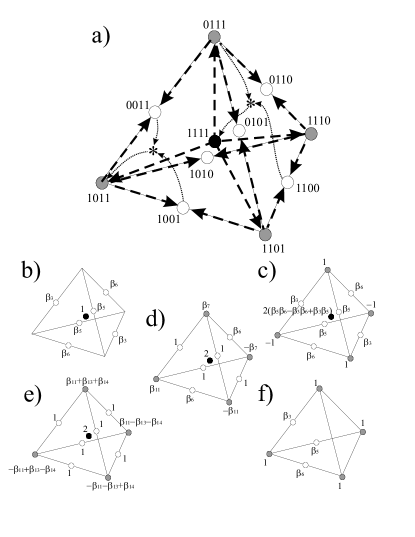
Figure 3: Diagram illustrating the dynamics of the coefficients $\beta_{i}$ of the nilpotential $f$ for a $4$-qubit system subject to $SL(2,\mathbb{C})$ transformations. The coefficients corresponding to quadric, cubic, and bilinear terms are shown by black, gray, and white circles, respectively. a) Flux directions. The $SL(2,\mathbb{C})$ transformations are applied in such a way, that the polynomials remain in the canonic form with respect to $su(2)$ transformations, with all linear terms $\beta_{i}\sigma_{i}^{+}=0$. The dashed arrows show the linear contributions of different states to the time derivatives of the neighboring states, and the dotted arrows jointed by asterisk depict two types of bilinear contributions. The other, similar terms may be constructed by symmetry. b) Canonic form for the generic state and for singular classes corresponding to one c), two d), three e), and four f) vanishing eigenvalues of the determinant Eq. (69).

III.4.3 Dynamic equations for the nilpotential and construction of $SU(2)$ and $SL(2,\mathbb{C})$ tanglemeters

The dynamic equation Eq. (59) suggests an algorithm for evaluation of the tanglemeter. This is based on the idea of feedback by adjusting the parameters $P_{i}$ of the local transformations in Eq. (59) in function of the current values of the tanglemeter’s coefficients. To this end, we fix the terms linear in $\sigma_{i}^{+}$ in the local Hamiltonian of Eq. (51) as

$$P_{i}^{-}=\left(P_{i}^{+}\right)^{\ast}=-\mathrm{i}\beta_{i}\,,$$ (61)

where

$$\beta_{i}=\left.\frac{\partial f}{\partial\sigma_{i}^{+}}\right|_{\sigma\longrightarrow 0}\,,$$ (62)

are the coefficients of the linear terms in the nilpotential at a given time. From Eqs. (59,61) we find the evolution of these coefficients under local transformations,

$$\frac{\partial\beta_{i}}{\partial t}=-\beta_{i}+\sum_{i=1}^{n}\bigg{[}\beta_{j}^{\ast}\left.\frac{\partial^{2}f}{\partial\sigma_{j}^{+}\partial\sigma_{i}^{+}}\right|_{\sigma\longrightarrow 0}-\beta_{i}\left|\beta_{i}\right|^{2}\bigg{]}\,.$$ (63)

When $f$ is close to $f_{c}$, the matrix of the second derivatives $M_{ij}=(\partial^{2}f/\partial\sigma_{j}^{+}\partial\sigma_{i}^{+})|_{\sigma\longrightarrow 0}$ can be explicitly expressed in terms of the “second excited state amplitudes”, $\psi_{0\ldots k_{i}=1,k_{j}=1,\ldots 0}$, which enter Eq. (8) and were introduced when discussing the $su$-canonic form of states. According to Eq. (17),

$$M_{ij}^{C}= \left.\frac{\partial^{2}f_{c}}{\partial\sigma_{j}^{+}\partial\sigma_{i}^{+}}\right|_{\sigma\longrightarrow 0}$$

$$= \beta_{ij}=\alpha_{ij}=\psi_{0\ldots k_{i}=1,k_{j}=1,\ldots 0}/\psi_{0,\ldots 0}\,.$$

The condition of the maximum reference state population for a state in the canonic form suggested by Eqs. (8-9) implies that the population increment,

$$\delta\rho_{\left|\mathrm{O}\right\rangle} =\left|\psi_{0\ldots 0}\right|^{2}\bigg{[}\bigg{|}1-\frac{1}{2}\sum_{i,j}g_{i}\left(\mathrm{e}^{2\mathrm{i}(\varphi_{i}+\varphi_{j})}M_{ij}+\delta_{ij}\right)g_{j}\bigg{|}^{2}-1\bigg{]}$$

$$=-{\rm Re}\left|\psi_{0\ldots 0}\right|^{2}\sum_{i,j}g_{i}\left(e^{2i(\varphi_{i}+\varphi_{j})}M_{ij}+\delta_{ij}\right)g_{j}\,,$$

is always negative. As the phases $\varphi_{i}$ are arbitrary, it follows that the eigenvalues of $M_{ij}$ lie within the unit circle and hence their real parts lie in the interval $(-1,1)$. Therefore the equation (63) linearized in the vicinity of the canonic state

$$\frac{\partial\beta_{i}}{\partial t} =-\beta_{i}+\sum_{j}M_{ij}\beta_{j}^{\ast}\,,$$

$$\frac{\partial\beta_{i}^{\ast}}{\partial t} =-\beta_{i}^{\ast}+\sum_{j}M_{ij}^{\ast}\beta_{j}\,,$$ (64)

has a stable stationary point at $\left\{\beta_{i}\right\}=0$, which implies that the coefficients $\beta_{i}$ standing in front of the linear terms $\beta_{i}\sigma_{i}^{+}$ in the nilpotential tend to zero exponentially. The presence of the nonlinear terms $\beta_{i}\left|\beta_{i}\right|^{2}$ yet accelerates this trend. Therefore, an arbitrary nilpotential $f$ subject to the local transformation with the parameters of the Hamiltonian Eq. (51) chosen according to the feedback conditions Eqs. (61,62), rapidly converges to the tanglemeter $f_{c}$. The problem of finding an efficient numerical algorithm for determining the tanglemeter for large assemblies is thereby solved. Verification that the outcome indeed corresponds to the global maximum of the reference state population should finalize the procedure. Note however, that the maximum vacuum state population obtained with local transformations corresponds to the maximum population of the ground state for each qubit. On the other hand, for a given set of single-qubit density matrices, the local operations maximizing the ground state population of each qubits are uniquely defined. Therefore, the only maximum of the reference state population is the global one, and hence, no matter what the initial state is, the procedure indeed converges to the canonic state and no verification is required.

A procedure of reducing the nilpotential to the canonic form can be carried out also for $SL$ transformations. At the first stage of this procedure, we reduce it to the $su$-canonic form so that the terms linear in $\sigma_{i}^{+}$ are absent. Then we apply $SL$ operations. An element of the $SL(2,\mathbb{C})$ group can be represented as $\exp\{it(P_{i}^{-}\sigma_{i}^{+}+P_{i}^{+}\sigma_{i}^{-}+P_{i}^{z}\sigma_{i}^{z})\}$, where $P_{i}^{-}$ and $P_{i}^{+}$ are no longer complex conjugates and $P_{i}^{z}$ is also a complex number.

Finding the $sl$-canonic state can also be formulated as a control problem, based on the feedback. We choose the parameters $P_{i}$ in the Hamiltonian Eq. (54) in such a way that the terms in the nilpotential involving the monomials of order one and of order $n-1$ in $\sigma_{i}^{+}$ would decrease exponentially with time. To this end, we may choose at this stage $P_{i}^{z}=0$ and impose two conditions, (i) the condition

$$P_{j}^{-}=-\sum_{i=1}^{n}\left.P_{i}^{+}\frac{\partial^{2}f}{\partial\sigma_{i}^{+}\partial\sigma_{j}^{+}}\right|_{\sigma\rightarrow 0}=-\sum_{i=1}^{n}P_{i}^{+}\beta_{i,j}\,,$$ (65)

expressing $P^{-}_{i}$ via $P^{+}_{i}$ which is keeping the nilpotential in the form of tanglemeter, and (ii) the condition

$$\left.\mathrm{i}\frac{\partial^{n-1}f}{{\textstyle\prod_{i\neq j}}\partial\sigma_{i}^{+}}\right|_{\sigma\rightarrow 0}=-P_{j}^{+}\frac{\partial^{n}f}{{\textstyle\prod_{i}}\partial\sigma_{i}^{+}}$$ (66)

$$+\sum_{m=1}^{n}P_{k}^{+}\left.\frac{\partial^{n-1}}{{\textstyle\prod_{i\neq m}}\partial\sigma_{i}^{+}}\left[\sigma_{i}^{+}\left(\frac{\partial f}{\partial\sigma_{i}^{+}}\right)^{2}\right]\right|_{\sigma\rightarrow 0}\,,$$

which ensures the exponential decrease of all $n$ coefficients in front of the second-highest order terms.

After having eliminated the monomials of orders $1$ and $n-1$, we can specify the scaling parameters $P_{i}^{z}$ such that $n$ additional conditions are imposed on the tangemeter coefficients. For example, one can set to unity the coefficients in front of the highest order term and set $(n-1)$ coefficients in front of certain monomials equal to $(n-1)$ coefficients of other monomials. Within the group $G$, multiplication by a complex number $\kappa\in\mathbb{C}^{*}$ allows one to normalize the canonic state to unit vacuum-state amplitude and thereby to get rid of the constant term in the $sl$-tanglemeter $f_{C}$ Eq. (25).

The condition Eq. (66) on $P_{j}^{+}$ is written implicitly as a set of $n$ linear equations. These equations can be resolved for generic states as we will show in the next section in the four-qubit example Eq. (67). However, they have no solution when the determinant of the system vanishes. These singularities correspond to singular classes of entangled states and require special consideration.

III.4.4 Example: Classes and $sl$-tanglemeters for $4$ qubits

Now with the examble of $4$-qubit assembly we illustrate the procedure of evaluation of the $sl$-tanglemeter with the help of dynamic equations supplimented by the feedback conditions. The $su$-tanglemeter Eq. (22) has 11 complex coefficients $\beta_{i}$ and one has to solve a system of eleven first-order nonlinear differential equations. Instead of presenting this awkward system explicitly, in Fig. 3 we schematically depict contributions to the time derivatives of the $\beta_{i}$ which are either linear or bilinear in the tanglemeter coefficients, and can be interpreted as a sort of “entanglement fluxes” Cubitt . One notices that the coupling of the second-order terms $\beta_{ij}\sigma_{i}^{+}\sigma_{j}^{+}$ to the fourth-order term $\beta_{15}\sigma_{4}^{+}\sigma_{3}^{+}\sigma_{2}^{+}\sigma_{1}^{+}$ occur via the third-order terms $\beta_{7}\sigma_{3}^{+}\sigma_{2}^{+}\sigma_{1}^{+}$, $\beta_{13}\sigma_{4}^{+}\sigma_{3}^{+}\sigma_{1}^{+}$, $\beta_{11}\sigma_{4}^{+}\sigma_{2}^{+}\sigma_{2}^{+}$, $\beta_{14}\sigma_{2}^{+}\sigma_{3}^{+}\sigma_{4}^{+}$, and thus the time evolution of all $\beta_{i}$ stops when this third-order coefficients $\beta_{7}$, $\beta_{13}$, $\beta$, and $\beta_{14}$ vanish. Therefore, by setting the time dependence of the parameters $P_{1}^{+}$, $P_{2}^{+}$, $P_{3}^{+}$ and $P_{4}^{+}$ such that they drive all four third-order coefficients to zero, we gradually reduce the $SU(2)$ canonic form of Eq. (22) to the $SL(2,\mathbb{C})$ form of Eq. (27). This control process results in an exponentially fast vanishing of the coefficients $\beta_{7}$, $\beta_{13}$, $\beta_{11}$, and $\beta_{14}$.

We now write down explicitly the differential equations for these coefficients,

$$\mathrm{i}\overset{.}{\beta}_{14} =\!-P_{1}^{+}\beta_{15}+2P_{2}^{+}\beta_{6}\beta_{10}+2P_{3}^{+}\beta_{6}\beta_{12}+2P_{4}^{+}\beta_{10}\beta_{12},$$

$$\mathrm{i}\overset{.}{\beta}_{13} =2P_{1}^{+}\beta_{5}\beta_{9}-P_{2}^{+}\beta_{15}+2P_{3}^{+}\beta_{5}\beta_{12}+2P_{4}^{+}\beta_{9}\beta_{12},$$

$$\mathrm{i}\overset{.}{\beta}_{11} =2P_{1}^{+}\beta_{3}\beta_{9}+2P_{2}^{+}\beta_{3}\beta_{10}-P_{3}^{+}\beta_{15}+2P_{4}^{+}\beta_{9}\beta_{10},$$

$$\mathrm{i}\overset{.}{\beta}_{7} =2P_{1}^{+}\beta_{3}\beta_{5}+2P_{2}^{+}\beta_{3}\beta_{6}+2P_{3}^{+}\beta_{5}\beta_{6}-P_{4}^{+}\beta_{15}\,,$$ (67)

and see that, in the general case, by a proper choice of the paremeters $P_{i}^{+}$ one can impose the feedback conditions such that these equations take the form

$$\overset{.}{\beta}_{7}=-\beta_{7};\quad\overset{.}{\beta}_{11}=-\beta_{11};\quad\overset{.}{\beta}_{13}=-\beta_{13};\quad\overset{.}{\beta}_{14}=-\beta_{14}\,.$$

The evolution implied by these equations brings the nilpotential in the form of $sl$-tanglemeter $f_{C}$. We note that the coefficients $P_{i}^{-}$ should satisfy the requirement Eq. (65) which ensures that the nilpotential always remains in the form of the tanglemeter $f_{c}$ during this evolution even if the state does not remain in the same $su$-orbit. We thus arrive at the tanglemeter $f_{C}$ of Eq. (27), defined up to the scaling factors. Now we can invoke the scaling of the nilpotent variables $\sigma_{i}^{+}$and reduce the tanglemeter $f_{c}$ to the $sl$-canonic form $f_{C}$ of Eq. (28), unless one of the bilinear coefficients vanish. The latter case corresponds to a measure-zero manifold and the canonic form may be chosen as

$$f_{C} =\sigma_{2}^{+}\sigma_{1}^{+}+\beta_{5}\left(\sigma_{3}^{+}\sigma_{1}^{+}+\sigma_{4}^{+}\sigma_{2}^{+}\right)$$ (68)

$$+\beta_{6}\left(\sigma_{4}^{+}\sigma_{1}^{+}+\sigma_{3}^{+}\sigma_{2}^{+}\right)+\sigma_{4}^{+}\sigma_{3}^{+}\sigma_{2}^{+}\sigma_{1}^{+},$$

or in any equivalent form resulting from a the permutation of the indices. More singular classes are discussed in Appendix B.

Reducing $f$ to the canonic forms of Eqs. (28,68) is unattainable when the determinant

$$\left|\begin{array}[c]{cccc}-\beta_{15}&2\beta_{6}\beta_{10}&2\beta_{6}\beta_{12}&2\beta_{10}\beta_{12}\\ 2\beta_{5}\beta_{9}&-\beta_{15}&2\beta_{5}\beta_{12}&2\beta_{9}\beta_{12}\\ 2\beta_{3}\beta_{9}&2\beta_{3}\beta_{10}&-\beta_{15}&2\beta_{9}\beta_{10}\\ 2\beta_{3}\beta_{5}&2\beta_{3}\beta_{6}&2\beta_{5}\beta_{6}&-\beta_{15}\end{array}\right|$$ (69)

vanishes, and it becomes impossible to impose the required feedback conditions. In that event, we loose control over the dynamics of $\beta_{7}$, $\beta_{13}$, $\beta_{11},$, and $\beta_{14}$, and some linear combinations of these coefficients cannot be set to zero by a proper choice of $P_{i}^{+}$. Consider this singular case in more detail. The determinant Eq. (69) is equal to zero when one or more of its eigenvalues,

$$\gamma_{1} =\beta_{15}-2\sqrt{\beta_{5}\beta_{6}\beta_{9}\beta_{10}}+2\sqrt{\beta_{3}\beta_{6}\beta_{9}\beta_{12}}-2\sqrt{\beta_{3}\beta_{5}\beta_{10}\beta_{12}}\,,$$

$$\gamma_{2} =\beta_{15}+2\sqrt{\beta_{5}\beta_{6}\beta_{9}\beta_{10}}-2\sqrt{\beta_{3}\beta_{6}\beta_{9}\beta_{12}}-2\sqrt{\beta_{3}\beta_{5}\beta_{10}\beta_{12}}\,,$$

$$\gamma_{3} =\beta_{15}-2\sqrt{\beta_{5}\beta_{6}\beta_{9}\beta_{10}}-2\sqrt{\beta_{3}\beta_{6}\beta_{9}\beta_{12}}+2\sqrt{\beta_{3}\beta_{5}\beta_{10}\beta_{12}}\,,$$

$$\gamma_{4} =\beta_{15}+2\sqrt{\beta_{5}\beta_{6}\beta_{9}\beta_{10}}+2\sqrt{\beta_{3}\beta_{6}\beta_{9}\beta_{12}}+2\sqrt{\beta_{3}\beta_{5}\beta_{10}\beta_{12}}\,,$$ (70)

vanish. Let us first focus on the case where only the first eigenvalue is zero. This implies that six coefficients in front of the bilinear terms and the coefficient $\beta_{15}$ in front of the $4$-order term are no longer independent parameters – the last one being the function of the first ones explicitly given by $\gamma_{1}=0$. The eigenvector

$$\left(-\sqrt{\beta_{6}\beta_{10}\beta_{12}},\sqrt{\beta_{5}\beta_{9}\beta_{12}},-\sqrt{\beta_{3}\beta_{9}\beta_{10}},\sqrt{\beta_{3}\beta_{5}\beta_{6}}\right)\,,$$

corresponding to $\gamma_{1}$ gives the combination of the cubic terms that cannot be eliminated,

$$-\lambda\sqrt{\beta_{6}\beta_{10}\beta_{12}}\sigma_{4}^{+}\sigma_{3}^{+}\sigma_{2}^{+}+\lambda\sqrt{\beta_{5}\beta_{9}\beta_{12}}\sigma_{4}^{+}\sigma_{3}^{+}\sigma_{1}^{+}$$

$$-\lambda\sqrt{\beta_{3}\beta_{9}\beta_{10}}\sigma_{4}^{+}\sigma_{2}^{+}\sigma_{1}^{+}+\lambda\sqrt{\beta_{3}\beta_{5}\beta_{6}}\sigma_{3}^{+}\sigma_{2}^{+}\sigma_{1}^{+}\,.$$

Clearly, this combination is determined up to a scaling factor $\lambda$. The nilpotential of Eq. (22) thus takes the form

$$f =\beta_{3}\sigma_{2}^{+}\sigma_{1}^{+}+\beta_{5}\sigma_{3}^{+}\sigma_{1}^{+}+\beta_{9}\sigma_{4}^{+}\sigma_{1}^{+}+\beta_{6}\sigma_{3}^{+}\sigma_{2}^{+}+\beta_{10}\sigma_{4}^{+}\sigma_{2}^{+}+\beta_{12}\sigma_{4}^{+}\sigma_{3}^{+}$$

$$+\lambda\left(\sqrt{\beta_{3}\beta_{5}\beta_{6}}\sigma_{3}^{+}\sigma_{2}^{+}\sigma_{1}^{+}-\sqrt{\beta_{3}\beta_{9}\beta_{10}}\sigma_{4}^{+}\sigma_{2}^{+}\sigma_{1}^{+}+\sqrt{\beta_{5}\beta_{9}\beta_{12}}\sigma_{4}^{+}\sigma_{3}^{+}\sigma_{1}^{+}-\sqrt{\beta_{6}\beta_{10}\beta_{12}}\sigma_{4}^{+}\sigma_{3}^{+}\sigma_{2}^{+}\right)$$

$$+2\left(\sqrt{\beta_{5}\beta_{6}\beta_{9}\beta_{10}}-\sqrt{\beta_{3}\beta_{6}\beta_{9}\beta_{12}}+\sqrt{\beta_{3}\beta_{5}\beta_{10}\beta_{12}}\right)\sigma_{4}^{+}\sigma_{3}^{+}\sigma_{2}^{+}\sigma_{1}^{+}\,,$$ (71)

specified in terms of seven complex parameters $\left(\lambda,\beta_{i}\right)$. We can eliminate four of these complex parameters by setting the scaling factors of $\sigma_{i}^{+}$, and arrive at the form

$$f_{C} =\beta_{3}\left(\sigma_{2}^{+}\sigma_{1}^{+}+\sigma_{4}^{+}\sigma_{3}^{+}\right)+\beta_{5}\left(\sigma_{3}^{+}\sigma_{1}^{+}+\sigma_{4}^{+}\sigma_{2}^{+}\right)$$

$$+\beta_{6}\left(\sigma_{4}^{+}\sigma_{1}^{+}+\sigma_{3}^{+}\sigma_{2}^{+}\right)$$

$$+\sigma_{3}^{+}\sigma_{2}^{+}\sigma_{1}^{+}-\sigma_{4}^{+}\sigma_{2}^{+}\sigma_{1}^{+}+\sigma_{4}^{+}\sigma_{3}^{+}\sigma_{1}^{+}-\sigma_{4}^{+}\sigma_{3}^{+}\sigma_{2}^{+}$$

$$+2\left(\beta_{5}\beta_{6}-\beta_{3}\beta_{6}+\beta_{3}\beta_{5}\right)\sigma_{4}^{+}\sigma_{3}^{+}\sigma_{2}^{+}\sigma_{1}^{+}\,,$$ (72)

which depends only on three complex parameters. This combination can be considered as a class of the polynomials that cannot be reduced to the canonic forms of Eqs. (28,68) by the sequential application of infinitesimal transformations preserving the canonic $SU(2)$ form. Permutation of indices of $\sigma_{i}^{+}$ give equivalent classes.

Next, we consider the case where two of the eigenvalues, say $\gamma_{1}$ and $\gamma_{2}$, of Eq. (70) are zero, that is,

$$\beta_{15}=2\beta_{3}\beta_{12}\,,\;\;\;\beta_{5}\beta_{10}=\beta_{3}\beta_{12}\,.$$

The corresponding eigenvectors

$$\left(-\sqrt{\beta_{6}\beta_{10}\beta_{12}},\sqrt{\beta_{5}\beta_{9}\beta_{12}},-\sqrt{\beta_{3}\beta_{9}\beta_{10}},\sqrt{\beta_{3}\beta_{5}\beta_{6}}\right)\,,$$

$$\left(-\sqrt{\beta_{6}\beta_{10}\beta_{12}},-\sqrt{\beta_{5}\beta_{9}\beta_{12}},\sqrt{\beta_{3}\beta_{9}\beta_{10}},\sqrt{\beta_{3}\beta_{5}\beta_{6}}\right)\,,$$

suggest the form of the nilpotential

$$f =\beta_{3}\sigma_{2}^{+}\sigma_{1}^{+}+\beta_{5}\sigma_{3}^{+}\sigma_{1}^{+}+\beta_{9}\sigma_{4}^{+}\sigma_{1}^{+}+\beta_{6}\sigma_{3}^{+}\sigma_{2}^{+}+\beta_{10}\sigma_{4}^{+}\sigma_{2}^{+}+\beta_{12}\sigma_{4}^{+}\sigma_{3}^{+}$$

$$+\lambda\left(\sqrt{\beta_{3}\beta_{5}\beta_{6}}\sigma_{3}^{+}\sigma_{2}^{+}\sigma_{1}^{+}-\sqrt{\beta_{3}\beta_{9}\beta_{10}}\sigma_{4}^{+}\sigma_{2}^{+}\sigma_{1}^{+}+\sqrt{\beta_{5}\beta_{9}\beta_{12}}\sigma_{4}^{+}\sigma_{3}^{+}\sigma_{1}^{+}-\sqrt{\beta_{6}\beta_{10}\beta_{12}}\sigma_{4}^{+}\sigma_{3}^{+}\sigma_{2}^{+}\right)$$

$$+\mu\left(\sqrt{\beta_{3}\beta_{5}\beta_{6}}\sigma_{3}^{+}\sigma_{2}^{+}\sigma_{1}^{+}+\sqrt{\beta_{3}\beta_{9}\beta_{10}}\sigma_{4}^{+}\sigma_{2}^{+}\sigma_{1}^{+}-\sqrt{\beta_{5}\beta_{9}\beta_{12}}\sigma_{4}^{+}\sigma_{3}^{+}\sigma_{1}^{+}-\sqrt{\beta_{6}\beta_{10}\beta_{12}}\sigma_{4}^{+}\sigma_{3}^{+}\sigma_{2}^{+}\right)$$

$$+2\beta_{3}\beta_{12}\sigma_{4}^{+}\sigma_{3}^{+}\sigma_{2}^{+}\sigma_{1}^{+},$$

which after a proper scaling can be simplified

$$f_{C} =\sigma_{2}^{+}\sigma_{1}^{+}+\sigma_{3}^{+}\sigma_{1}^{+}+\sigma_{4}^{+}\sigma_{2}^{+}+\sigma_{4}^{+}\sigma_{3}^{+}+\beta_{6}\left(\sigma_{4}^{+}\sigma_{1}^{+}+\sigma_{3}^{+}\sigma_{2}^{+}\right)$$

$$+\beta_{7}\left(\sigma_{3}^{+}\sigma_{2}^{+}\sigma_{1}^{+}-\sigma_{4}^{+}\sigma_{3}^{+}\sigma_{2}^{+}\right)+\beta_{11}\left(\sigma_{4}^{+}\sigma_{2}^{+}\sigma_{1}^{+}-\sigma_{4}^{+}\sigma_{3}^{+}\sigma_{1}^{+}\right)$$

$$+2\sigma_{4}^{+}\sigma_{3}^{+}\sigma_{2}^{+}\sigma_{1}^{+}\,.$$ (73)

Again, this depends on three complex parameters and leads to equivalent classes under indices permutations.

Similarly, the case where $\gamma_{1}=\gamma_{2}=\gamma_{3}=0$ yields

$$\beta_{15}/2=\sqrt{\beta_{5}\beta_{10}}=\sqrt{\beta_{3}\beta_{12}}=\sqrt{\beta_{6}\beta_{9}}\,,$$

which after scaling results in

$$f_{C} =\sigma_{2}^{+}\sigma_{1}^{+}+\sigma_{3}^{+}\sigma_{1}^{+}+\sigma_{4}^{+}\sigma_{2}^{+}+\sigma_{4}^{+}\sigma_{3}^{+}+\sigma_{4}^{+}\sigma_{1}^{+}+\sigma_{3}^{+}\sigma_{2}^{+}$$

$$+\beta_{14}\left(\sigma_{3}^{+}\sigma_{2}^{+}\sigma_{1}^{+}-\sigma_{4}^{+}\sigma_{2}^{+}\sigma_{1}^{+}+\sigma_{4}^{+}\sigma_{3}^{+}\sigma_{1}^{+}-\sigma_{4}^{+}\sigma_{3}^{+}\sigma_{2}^{+}\right)$$

$$+\beta_{13}\left(\sigma_{3}^{+}\sigma_{2}^{+}\sigma_{1}^{+}+\sigma_{4}^{+}\sigma_{2}^{+}\sigma_{1}^{+}-\sigma_{4}^{+}\sigma_{3}^{+}\sigma_{1}^{+}-\sigma_{4}^{+}\sigma_{3}^{+}\sigma_{2}^{+}\right)$$

$$+\beta_{11}\left(\sigma_{3}^{+}\sigma_{2}^{+}\sigma_{1}^{+}-\sigma_{4}^{+}\sigma_{2}^{+}\sigma_{1}^{+}-\sigma_{4}^{+}\sigma_{3}^{+}\sigma_{1}^{+}+\sigma_{4}^{+}\sigma_{3}^{+}\sigma_{2}^{+}\right)$$

$$+2\sigma_{4}^{+}\sigma_{3}^{+}\sigma_{2}^{+}\sigma_{1}^{+}\,.$$ (74)

The last case, where all four $\gamma_{i}=0$, may be realized by setting to zero just three parameters, say $\beta_{15}=\beta_{10}=\beta_{12}=0$. This enables us to dynamically eliminate one more of the bilinear coefficients, say $\beta_{9}$, and to set all the third-order coefficients equal to one by scaling. This yields a singular canonic form,

$$f_{C} =\sigma_{3}^{+}\sigma_{2}^{+}\sigma_{1}^{+}+\sigma_{4}^{+}\sigma_{3}^{+}\sigma_{1}^{+}+\sigma_{4}^{+}\sigma_{2}^{+}\sigma_{1}^{+}+\sigma_{4}^{+}\sigma_{3}^{+}\sigma_{2}^{+}$$

$$+\beta_{3}\sigma_{2}^{+}\sigma_{1}^{+}+\beta_{5}\sigma_{3}^{+}\sigma_{1}^{+}+\beta_{6}\sigma_{3}^{+}\sigma_{2}^{+},$$ (75)

which still depends on three parameters and allows permutations. All five $sl$-tanglemeters obtained from the dynamic equations and dependent on three complex parameters are depicted in Fig. 3.

IV Entanglement beyond qubits

In this section we show how the nilpotent polynomials approach may be extended to describe situations more general than assemblies of qubits. In particular, we discuss in detail the case of qutrits, each qutrit being transformed by $SU(3)$ or $SL(3,\mathbb{C})$ groups, and construct appropriate nilpotent polynomials $F$ and $f=\ln F$ for these systems. We define the canonic form $F_{c}$ for $F$ and the tanglemeter $f_{c}$. Next, we generalize this technique to qudits $d$-level elements–qudits.

Remarkably, the nilpotent polynomials formalism allows us to make contact with the framework of generalized entanglement, introduced in Refs. Barnum1 ; Barnum2 . While the latter provides a notion of entanglement which relies directly on physical observables and, as such, is meaningful even in the absence of an underlying system partition (see also GE ), an important special case arises in the situations where an element structure is specified, but, due to some operational or fundamental constraint, the rank $r$ of the algebra of local transformations is smaller than $d-1$, where $d$ is the element dimension. In this context, special attention is devoted to spin-$1$ systems, namely three-level systems restricted to evolve under the action of spin operators living in the $so(3)\equiv su(2)$ subalgebra of $su(3)$. In particular, we show how to introduce nilpotent polynomials for characterizing generalized entanglement within a single element of an assembly. In such a case, one encounters a new kind of the nilpotent variables whose squares do not vanish and only some higher powers do. We also consider entanglement among different elements of such an assembly.

We conclude by extending the nilpotent polynomials formalism to the case of multipartite entanglement among groups of elements comprising the assembly, that is, to the case where different elements of an assembly merge, thereby creating a new assembly with elements of higher dimensions.

IV.1 Qutrits and qudits

In order to describe entanglement among $d$-level elements of an assembly, one needs to invoke the Lie algebras of higher rank $su(d)$ and their complex versions $sl(d,\mathbb{C})$. The construction of nilpotent polynomials for such systems is based on the so-called Cartan-Weyl decomposition. We illustrate this for qutrits, $d=3$, and then generalize to arbitrary $d$.

IV.1.1 Nilpotent variables for qutrits

Let us start by reminding some basic facts about group theory and Lie algebra representation theory Cornwell ; Humphreys . The $d^{2}-1$ generators of the algebra $sl(d)$, the complexified $su(d)$, may be decomposed into 3 sets:

(i)

a set $\mathcal{H}$ of $r=d-1$ linearly independent, mutually commuting generators of a Cartan subalgebra span($\mathcal{H}$) ($r$ is the rank of the algebra and span($\mathcal{H}$) is the vector space spanned by $\mathcal{H}$). In a faithful matrix representation, the most natural choice for Cartan generators are traceless $d\times d$ diagonal matrices.

(ii)

a set $\{\mathcal{E}\}$ of $d(d-1)/2$ “raising” generators spanning a nilpotent subalgebra span($\mathcal{E})\subset su(d)$. The elements of $\{\mathcal{E}\}$ and of span($\mathcal{E})$ can be represented by the matrices with nonzero elements only above the main diagonal.

(iii)

$d(d-1)/2$ Hermitian conjugate “lowering” generators spanning a nilpotent subalgebra span$\{\mathcal{F}\}$ represented by matrices with nonzero elements only below the diagonal.

In the case of $su(2)$, each of the above sets contains a single generator: $\mathcal{H}=\{\sigma^{3}=\sigma_{z}\},\ \mathcal{E}=\{\sigma^{+}\}$ and $\mathcal{F}=\{\sigma^{-}\}$. For $su(3)$ having eight generators represented by the eight Gell-Mann $\lambda^{a}$ matrices Cornwell , the Cartan subalgebra involves two generators usually chosen as

$$\begin{array}[c]{cc}\lambda^{3}=\left(\begin{array}[c]{ccc}1&0&0\\ 0&-1&0\\ 0&0&0\end{array}\right),&\lambda^{8}=\dfrac{1}{\sqrt{3}}\left(\begin{array}[c]{ccc}1&0&0\\ 0&1&0\\ 0&0&-2\end{array}\right).\end{array}$$ (76)

The basis $\mathcal{E}$ for the raising nilpotent subalgebra is comprised of $3$ elements,

$$s^{+}=\frac{\lambda^{1}+i\lambda^{2}}{2}=\left(\begin{array}[c]{ccc}0&1&0\\ 0&0&0\\ 0&0&0\end{array}\right),$$ (77)

$$u^{+}=\frac{\lambda^{4}+i\lambda^{5}}{2}=\left(\begin{array}[c]{ccc}0&0&1\\ 0&0&0\\ 0&0&0\end{array}\right),$$ (78)

$$t^{+}=\frac{\lambda^{6}+i\lambda^{7}}{2}=\left(\begin{array}[c]{ccc}0&0&0\\ 0&0&1\\ 0&0&0\end{array}\right),$$ (79)

while $\mathcal{F}$ includes their Hermitian conjugates.

The elements of $\mathcal{E}$ and $\mathcal{F}$ are the root vectors of $su(3)$. It means that for $e\in\mathcal{E}$, $f\in\mathcal{F}$, and $h\in{\sl span}(\mathcal{H})$, the commutator $[e,h]$ is proportional to $e$, and the commutator $[f,h]$ is proportional to $f$. The subalgebra $\mathcal{E}$ is nilpotent, meaning that the multiple commutators $[e_{1},\ldots,[e_{p-1},e_{p}]\ldots]$ vanish starting at some level $p-1$. For $su(3)$ with only one nontrivial commutator $[s^{+},t^{+}]=u^{+}$, double commutators already vanish. For $su(d)$, they vanish at the level $d-1$, coinciding with the rank of the algebra $r$.

A generic pure state of a qutrit may be represented as

$$|\psi\rangle=\psi_{0}|0\rangle+\psi_{1}|1\rangle+\psi_{2}|2\rangle=\left(\psi_{0}+\psi_{1}t^{+}+\psi_{2}u^{+}\right)|0\rangle\,,$$ (80)

with

$$|0\rangle\equiv\left(\begin{array}[]{c}0\\ 0\\ 1\end{array}\right),\;|1\rangle\equiv\left(\begin{array}[]{c}0\\ 1\\ 0\end{array}\right),\;|2\rangle\equiv\left(\begin{array}[]{c}1\\ 0\\ 0\end{array}\right).$$ (81)

Equation (80) generalizes a similar representation for the qubit pure states extensively discussed so far. The operators $t^{+},u^{+}$ belong to $\mathcal{E}$ and commute. Note that even for larger $d$, such a set of $d-1=r$ commuting nilpotent operators always exists note2 , allowing one to express a generic qudit state as a first-order polynomial of commuting nilpotent variables.

The state $|0\rangle$, which by definition is annihilated by all “lowering” generators of ${\cal F}$, plays the special role of the Fock vacuum or reference state. But the choice Eq. (81) is not unique. Actually, any qutrit state can serve as a valid reference state. For each $|\tilde{0}\rangle=U|0\rangle,\ U\in SU(3)$, the analysis above applies if one merely changes (conjugates) accordingly the Cartan-Weyl decomposition and defines

$$\tilde{\cal H}=U{\cal H}U^{-1}\,,\;\;\tilde{\cal E}=U{\cal E}U^{-1}\,,\;\;\tilde{\cal F}=U{\cal F}U^{-1}\,.$$

Again, span($\tilde{\mathcal{E}}$) and span($\tilde{\mathcal{F}}$) are nilpotent; again, $|\tilde{0}\rangle$ are annihilated by the elements of $\tilde{\cal F}$, etc. For example, if the choice $|\tilde{0}\rangle=|1\rangle$ is made, the elements of ${\cal E}$ are $\tilde{s}^{+}=-u^{+},\tilde{t}^{+}=-t^{-},\tilde{u}^{+}=s^{+}$. In this case, a generic qutrit state would be expressed as

$$|\psi\rangle=\left(-\psi_{0}\tilde{t}^{+}+\psi_{1}+\psi_{2}\tilde{u}^{+}\right)|1\rangle\ =\left(\psi_{0}t^{-}+\psi_{1}+\psi_{2}s^{+}\right)|1\rangle\,,$$ (82)

The choice of Eq. (80) is more natural for discussing qutrits, whereas the choice made in Eq. (82) allows one to associate $\lambda^{3}$ with the spin projection operator $S_{z}$ for a spin-$1$ system, with the vacuum state $|\tilde{0}\rangle=|1\rangle$ naturally corresponding to the lowest eigenvalue $-1$ of this operator. The state $|1\rangle$ is so-called extremal weight state for the representation and is discussed in Sect. IVC in more details. In any case, this choice is mainly a matter of state labeling, which in most cases is dictated by convenience and can then be done accordingly for each particular physical problem.

In analogy with Eq. (13), the state of $n$ qutrits can then be written as

$$|\Psi\rangle =\ \sum_{\{\nu_{i},\eta_{i}=0,1\,/\nu_{i}\eta_{i}=0\}}\psi_{2\nu_{n}+\eta_{n}\ldots 2\nu_{1}+\eta_{1}}\prod_{i=1}^{n}(u_{i}^{+})^{\nu_{i}}(t_{i}^{+})^{\eta_{i}}|\mathrm{O}\rangle$$

$$=F(u_{i}^{+},t_{i}^{+})|\mathrm{O}\rangle\ ,$$ (83)

where $|\mathrm{O}\rangle=|0,\ldots,0\rangle$ denotes the reference state. Our next steps are: (i) to consider the nilpotential $f=\ln F$; (ii) to bring it into the canonic form specified by the requirement of maximum population of the state $|\mathrm{O}\rangle$ followed by the requirement of maximum population of the state $\left|1\right\rangle=\left|1\ldots 1\right\rangle$, as discussed at the end of Sect. II.1; and (iii) to normalize $|\Psi_{C}\rangle$ by the condition $\langle\mathrm{O}|\Psi_{C}\rangle=1$. The tanglemeter $f_{C}$ thereby obtained provides one with simple entanglement characteristics and relevant insights. Let us explain how this construction works for an assembly of two qutrits.

IV.1.2 Entanglement of two qutrits

We select $|\mathrm{O}\rangle=|0,0\rangle$ as the reference state. The relevant nilpotent variables are $u_{i}^{+}$ and $t_{i}^{+}$, where the index $i=1,2$ labels the qutrits. An arbitrary assembly state can then be written as

$$|\Psi\rangle =F(u_{i}^{+},t_{i}^{+})|\mathrm{O}\rangle=(\psi_{00}+\psi_{01}t_{1}^{+}$$

$$+\psi_{02}u_{1}^{+}+\psi_{10}t_{2}^{+}+\psi_{20}u_{2}^{+}+\psi_{11}t_{1}^{+}t_{2}^{+}$$

$$+\psi_{12}t_{2}^{+}u_{1}^{+}+\psi_{21}u_{2}^{+}t_{1}^{+}+\psi_{22}u_{2}^{+}u_{1}^{+})|\mathrm{O}\rangle\>.$$ (84)

The requirement of maximum population of $|\mathrm{O}\rangle$ dictates that the linear terms in $F(u_{i}^{+},t_{i}^{+})$ vanish. This is proved by inspecting the variation of the population under local unitary transformations, similarly to what was done for qubits (see Eq. (8)). Imposing also our normalization constraint dictating that the expansion of $F$ starts with $1$, we bring $F_{c}$ into the form

$$F_{c}=1+\alpha_{11}t_{2}^{+}t_{1}^{+}+\alpha_{12}t_{2}^{+}u_{1}^{+}+\alpha_{21}u_{2}^{+}t_{1}^{+}+\alpha_{22}u_{2}^{+}u_{1}^{+}\,.$$ (85)

Thus, we are left with the reference state and four excited states. The form in Eq. (85) is invariant with respect to the subgroup $SU_{2}(2)\otimes SU_{1}(2)$ of local transformations which can mix the levels $|1\rangle$ and $|2\rangle$ for each qutrit, but preserve the population of the state $|\mathrm{O}\rangle$. Using this freedom, we further restrict the canonic form by acting on $|\Psi\rangle$ with the transformations of $SU_{2}(2)\otimes SU_{1}(2)$ that maximizes the population of the state $|11\rangle=t_{2}^{+}t_{1}^{+}|0\rangle$, while the population of the reference state $|\mathrm{O}\rangle$ is already maximized. This eliminates the terms $\propto t_{2}^{+}u_{1}^{+}$ and $\propto u_{2}^{+}t_{1}^{+}$ in $F_{c}$. Thus, we finally obtain

$$F_{c}(u_{2}^{+},t_{2}^{+},u_{1}^{+},t_{1}^{+})=1+\alpha_{11}t_{2}^{+}t_{1}^{+}+\alpha_{22}u_{2}^{+}u_{1}^{+}\>.$$ (86)

The polynomial $F_{c}$ depends only on two complex parameters $\alpha_{ii}$, which can be set real and positive by a local phase transformation,

$$\exp\left(i\gamma_{2}\lambda_{2}^{3}+i\delta_{2}\lambda_{2}^{8}+i\gamma_{1}\lambda_{1}^{3}+i\delta_{1}\lambda_{1}^{8}\right).$$ (87)

Thus, two real parameters are sufficient for characterizing entanglement between two qutrits, as illustrated in Fig. 1 b). This is consistent with the result obtained by a straightforward application of the bipartite Schmidt decomposition.

When counting the number of invariants $N_{I}$  for a two-qutrit state with the help of the expression

$$D_{su}=2\cdot 3^{n}-8n-2\>,$$ (88)

we find $N_{I}=0$ for $n=2$. As for the two-qubit case, this number differs from the actual number of independent parameters because the phase transformation of Eq. (87) has more parameters than the number of the coefficients in Eq. (85), and some of them act on the coefficients in the same way (cf. Eq. (II.1) and the discussion thereabout). The counting given by Eq. (88) holds for $n\geq 3$.

IV.1.3 Entanglement in a generic qudit assembly

The above analysis suggests the following generalization to an assembly of $n$ qudits. Let $d_{i}$ denote the local dimension of the $i$-th element with the associated $su(d_{i})$ algebra. For each element $i$, we choose a reference state $|0\rangle_{i}$ and perform the corresponding Cartan-Weyl decomposition ${\cal H}_{i}\oplus{\cal E}_{i}\oplus{\cal F}_{i}$ for the generators of this algebra, in such a way that $f|0\rangle_{i}=0$ for all $f\in{\cal F}_{i}$). The most convenient choice for $|0\rangle_{i}$ is the state with only the lowest level occupied. One may choose a basis in the qudit Hilbert space involving the vacuum state $|0\rangle_{i}$ and the “excited states”, such that each basis state represents a joint eigenstate of all generators $\lambda_{i}^{\kappa_{i}}$ in the Cartan subalgebra ($\kappa_{i}=1,\ldots,d_{i}-1$). The eigenvalues of $\left\{\lambda_{i}^{\kappa_{i}}\right\}$ thus provide good quantum numbers labeling the qudit state.

Next, we choose a set of commuting nilpotent generators $\left\{\nu_{i}^{\kappa_{i}}\right\}\subseteq{\cal E}_{i}$ that may be employed as nilpotent variables. To be specific, let us enumerate these variables such that $\left|1\right\rangle_{i}=\nu_{i}^{1}\left|0\right\rangle_{i}$ corresponds to the first excited state of $i$-th element, $\left|2\right\rangle_{i}=\nu_{i}^{2}\left|0\right\rangle_{i}$ to the second, etc, A polynomial $F\left\{\nu_{i}^{\kappa_{i}}\right\}$ of these nilpotent arguments characterizes a generic quantum state of the assembly as the latter may be obtained acting by the operator $F$ on the corresponding assembly reference state $\left|\mathrm{O}\right\rangle={\textstyle\prod\nolimits_{i}}\left|0\right\rangle_{i}$.

In analogy with the procedure for two qutrits described above, we can, using local $SU(d_{i})$ operations, maximize the population of the vacuum state and eliminate the terms linear in the nilpotent operators. The function $F$ acquires the form generalizing Eq. (85),

$$F=1+\alpha_{ij}^{\kappa_{i}\kappa_{j}}\nu_{i}^{\kappa_{i}}\nu_{j}^{\kappa_{j}}+\alpha_{ijk}^{\kappa_{i}\kappa_{j}\kappa_{k}}\nu_{i}^{\kappa_{i}}\nu_{j}^{\kappa_{j}}\nu_{k}^{\kappa_{k}}\ldots,$$ (89)

where repeated indices imply summation. The state is normalized to unit amplitude of the reference state, as earlier. As a next step, we maximize the population of the symmetric state $|1,\ldots,1\rangle$ using the transformations of the subgroup $\otimes_{i}SU(d_{i}-1)$, where the tensor product is taken over all $i$ with $d_{i}>2$, which preserve the reference state. At the third step, we maximize the population of the state $|\{k_{i}\}\rangle$, where $k_{i}=2$ for the elements with $d_{i}>2$ while for qubits the label $k_{i}$ is “frozen” at the value $k_{i}=1$, and maximization is done using the transformations of the subgroup $\otimes_{i}SU(d_{i}-2)$ that affect neither the reference state nor the first excited state, and the tensor product involves now the elements with $d_{i}>3$. If the assembly involves 5-level elements, we are allowed at the next step to maximize the population of the state $|\{k_{i}\}\rangle$, where $k_{i}=1$ for qubits, $k_{i}=2$ for qutrits and $k_{i}=3$ for the elements with $d_{i}>3$, etc.

For example, for an assembly of a five-level system, a four-level system, and a qutrit, one should consecutively maximize:

(i) the population of the state $|0,0,0\rangle$ by the transformations from $SU(5)\otimes SU(4)\otimes SU(3)$;

(ii) the population of the state $|1,1,1\rangle$ by the transformations from $SU(4)\otimes SU(3)\otimes SU(2)$;

(iii) the population of the state $|2,2,2\rangle$ by the transformations from $SU(3)\otimes SU(2)$;

(iv) the population of the state $|3,3,2\rangle$ by the transformations from the remaining $SU(2)$ mixing the 3-d and the 4-th excited states of the five-level system.

This is all illustrated in Fig. 4.

This procedure eventually reduces the nilpotent polynomial $F$ to the canonic form of Eq. (89), where some coefficients $\alpha_{ij}^{\kappa_{i}\kappa_{j}}$, $\alpha_{ijk}^{\kappa_{i}\kappa_{j}\kappa_{k}}$ now vanish. In order to better understand the pattern, consider two examples: an assembly of three qutrits, and of two qutrits and a qubit. In the first case, the canonic form is

$$F_{c} =1+\alpha_{011}t_{2}^{+}t_{1}^{+}+\alpha_{012}t_{2}^{+}u_{1}^{+}+\alpha_{021}u_{2}^{+}t_{1}^{+}+\alpha_{022}u_{2}^{+}u_{1}^{+}+\alpha_{101}t_{3}^{+}t_{1}^{+}+\alpha_{102}t_{3}^{+}u_{1}^{+}+\alpha_{201}u_{3}^{+}t_{1}^{+}+\alpha_{202}u_{3}^{+}u_{1}^{+}+\alpha_{110}t_{3}^{+}t_{2}^{+}$$

$$+\alpha_{120}t_{3}^{+}u_{2}^{+}+\alpha_{210}u_{3}^{+}t_{2}^{+}+\alpha_{220}u_{3}^{+}u_{2}^{+}+\alpha_{111}t_{3}^{+}t_{2}^{+}t_{1}^{+}+\alpha_{122}t_{3}^{+}u_{2}^{+}u_{1}^{+}+\alpha_{212}u_{3}^{+}t_{2}^{+}u_{1}^{+}+\alpha_{221}u_{3}^{+}u_{2}^{+}t_{1}^{+}+\alpha_{222}u_{3}^{+}u_{2}^{+}u_{1}^{+}\,,$$ (90)

whereas for two qutrits and a qubit (labeled by the index 3), it looks as follows

$$F_{c}=1+\alpha_{4}t_{2}^{+}t_{1}^{+}+\alpha_{5}t_{2}^{+}u_{1}^{+}+\alpha_{7}u_{2}^{+}t_{1}^{+}+\alpha_{8}u_{2}^{+}u_{1}^{+}+\alpha_{10}t_{3}^{+}t_{1}^{+}+\alpha_{11}t_{3}^{+}u_{1}^{+}+\alpha_{12}t_{3}^{+}t_{2}^{+}+\alpha_{15}t_{3}^{+}u_{2}^{+}+\alpha_{13}t_{3}^{+}t_{2}^{+}t_{1}^{+}+\alpha_{17}t_{3}^{+}u_{2}^{+}u_{1}^{+}\,,$$ (91)

with the identification $\nu_{i}^{1}=t_{i}^{+}$ and $\nu_{i}^{2}=u_{i}^{+}$. In Eq. (90), the indices of $\alpha$ explicitly label the individual states of the qutrits, while in Eq. (91) the notation relies on the decimal representation of the base-$3$ numbers associated with these indices, $112\rightarrow 14$, etc. The canonic forms are defined, as before, up to phase factors of the nilpotent variables $\nu_{j}^{\kappa_{j}}$.

The forms of Eqs. (90,91) do not involve linear terms. Neither do they involve any term proportional to $t_{3}^{+}t_{2}^{+}u_{1}^{+},\ t_{3}^{+}u_{2}^{+}t_{1}^{+}$, and (for three qutrits) $u_{3}^{+}t_{2}^{+}t_{1}^{+}$. In other words, the amplitudes of the states $|1,1,2\rangle,\ |1,2,1\rangle$ and, for three qutrits, $|2,1,1\rangle$ vanish. This vanishing is achieved at the second stage of our procedure maximizing the population of the state $|1,1,1\rangle$ by the transformations from $\otimes_{i=1}^{3}SU(2)_{i}$ for three qutrits, and from $SU_{2}(2)\otimes SU_{1}(2)$ for two qutrits and a qubit. Indeed, from the viewpoint of the remaining $SU(2)$ transformations, the state $|1\rangle$ may be regarded as a reference state, and amplitudes like $|1,1,2\rangle$ vanish for the same reason why the amplitudes $|1,0,\ldots,0\rangle$ vanished when the population of $|{\Large O}\rangle$ were maximized. It is clear that, e.g., for an assembly of three four-level systems, where the procedure involves 3 steps, the canonic state has vanishing coefficients of the basis states $|2,1,1\rangle,|1,2,1\rangle,|1,1,2\rangle,|3,1,1\rangle,|1,3,1\rangle,|1,1,3\rangle,|3,2,2\rangle$,
$|2,3,2\rangle$ and $|2,2,3\rangle$. Generally, if the procedure involves the maximization of the population of the state $|\{k_{i}\}\rangle$, the vanishing amplitudes are $|\{k_{i}^{\prime}\}\rangle$, where the sets $\{k_{i}\}$ and $\{k_{i}^{\prime}\}$ differ only in one position $i_{0}$ and $k_{i_{0}}^{\prime}>k_{i_{0}}$.

Going back to Eq. (90), we observe that the canonic polynomial depends in this case on $17$ complex parameters, $6$ of which can be set real by a proper choice of the phase factors of the nilpotent variables $u_{i}^{+}$ and $t_{i}^{+}$. This coincides with the number $N_{I}=28$ suggested by the asymptotic formula given in Eq. (88) valid for $n>2$.

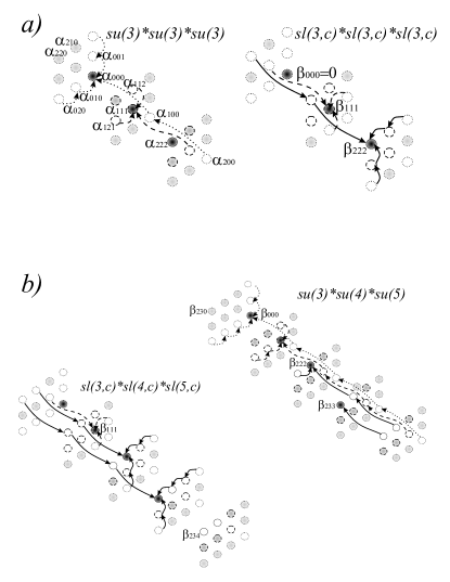
Figure 4: a)A possible strategy for identifying the tanglemeter $f_{c}$ for three qutrits. The choice of the parameters $P_{i}^{\kappa}$ of local unitary transformations is done in such a way that the transformations sequentially eliminate the terms in $F_{c}$ that are coupled to the states $\left|k,k,k\right\rangle$ by just one local operator. The $SU(3)$ transformations maximize the population of the vacuum $|\mathrm{O}\rangle=\left|0,0,0\right\rangle$. Next, the $SU(2)$ transformations not acting on the states $|0_{i}\rangle$ shown by dotted circles, and only the states shown by dashed and solid circle are mixed, maximize the population of the state $\left|1,1,1\right\rangle$. The population of the state $\left|2,2,2\right\rangle$ cannot be further maximized by local unitary operations. However, $SL(3)$ and $SL(2)$ dynamic transformations can eliminate some of the coefficients $\beta$ directly connected to such states. b) The same diagrams for the case of different elements.

The coefficients $\alpha_{i\ldots j}^{\kappa_{i}\ldots\kappa_{j}}$ can be treated as invariants characterizing the qudit entanglement. But the coefficients of the tanglemeter $f_{c}=\ln F_{c}$ provide, as we already saw, a more direct and physical description. In particular, the criterion of Eq. (18), indicating whether two groups, $A$ and $B$, of a bipartition are entangled, may be straightforwardly generalized. We have

$$\frac{\partial^{2}f(\{\nu_{i}^{\kappa_{i}}\})}{\partial\nu_{i}^{\kappa_{i}}\partial\nu_{m}^{\kappa_{m}}}=0,\;\;\;i\in A,\quad m\in B\,.$$

As before, this criterion holds even for a noncanonic nilpotential.

The construction of the $sl$-tanglemeter may be accomplished by analogy to the qubit case. One can derive and directly employ the dynamic equations for $f$, eliminate the states adjacent in the sense explained above to $\left|k,\ldots,k\right\rangle$ by a proper choice of the transformation parameters $P_{i}^{\kappa}$, thereby obtaining the $sl$-canonic form:

$$f_{C}=\beta_{ij}^{\kappa_{i}\kappa_{j}}\nu_{i}^{\kappa_{i}}\nu_{j}^{\kappa_{j}}+\ldots$$ (92)

Like it was the case for the $su$-tanglemeter, many of the coefficients $\beta_{ij}^{\kappa_{i}\kappa_{j}}$, $\beta_{ijk}^{\kappa_{i}\kappa_{j}\kappa_{k}}$, etc vanish, however. Actually, as $SL$ transformations have more parameters than $SU$-transformations, we can now bring to zero more coefficients than in the $SU$ case. Namely, the sum on the right hand side of Eq.(92) contains no terms corresponding to the states directly coupled to $\left|k,\ldots,k\right\rangle$ by any single local transformation, and not only those involving “higher” states with $k^{\prime}\geqslant k$ (for simplicity, we discuss here only the case when all elements have the same dimension). Without explicitly presenting the corresponding dynamic equations, we illustrate this idea in Fig. 4 for the case of qutrits. As one can see there, the generic $SL(3,\mathbb{C})$ canonic form of $f$ contains $8$ complex parameters, $6$ of which may be specified by a proper choice of the scaling factors. Thus,

$$f_{C} =\beta_{g}\left(u_{3}^{+}t_{2}^{+}+u_{2}^{+}t_{1}^{+}+t_{3}^{+}u_{1}^{+}\right)+t_{3}^{+}t_{2}^{+}t_{1}^{+}$$

$$+\beta_{u}\left(t_{2}^{+}u_{1}^{+}+u_{3}^{+}t_{1}^{+}+t_{3}^{+}u_{2}^{+}\right)+u_{3}^{+}u_{2}^{+}u_{1}^{+}\>.$$

IV.2 Generalized entanglement and generating functions

We now consider a situation where the local operations available for qudits are restricted by some operational or fundamental constraint, so that they cannot ensure universal local transformations. In particular, we focus on the case where the restricted local operations form a subgroup $SU(m)\subset SU(d)$, with $m<d$, of the full unitary transformation set. As mentioned, this is a special relevant instance of a more general, subsystem-independent entanglement setting (generalized entanglement) formalized in Refs. Barnum1 ; Barnum2 . One of the main implications of the latter approach is, in turn, to point to an intimate connection between entanglement and so-called generalized coherent states (GCSs) Perelomov ; Zhang , which is also useful to place our current analysis in a broader context.

Generalized coherent states may be constructed for quantum systems described by a dynamic-symmetry Lie group, which typically is assumed to be reductive or semisimple: a family of GCSs may be thought of as an orbit resulting from application of the Lie group to a reference state, which is identified with an extremal-weight state in the irreducible representation of the underlying dynamical Lie algebra. Within this general setting, the canonical coherent states of a quantum harmonic-oscillator Glauber may be recovered as resulting from the application of the displacement operator $[\exp\left(az^{\ast}-a^{\dagger}z\right)]$ to the ground state $\left|0\right\rangle$. Here, as usual, $a$ and$\ a^{\dagger}$ denote annihilation and creation operators, respectively, and $z=x+\mathrm{i}p\in{\mathbb{C}}$ stands for displacement in the phase space $\left(x,p\right)$. The relevant dynamic groups are generated by the Heisenberg-Weyl algebras, either $\mathfrak{h}_{3}=\{\mathbb{I},a,a^{\dagger}\}$ that allows for arbitrary displacements, or $\mathfrak{h}_{4}=\{\mathbb{I},a,a^{\dagger},a^{\dagger}a\}$ that in addition involves the phase space rotation $\exp\left(\mathrm{i}\varphi a^{\dagger}a\right)$ by an angle $\varphi$ note4 . Physically, the most representative manifestation of the coherent states is the fact that external interventions realized via $a{\dagger}$ and $a$ cannot change the structure of the wave function expressed in terms of the Wigner function, but just displace and rotate it in the phase space. One can also include the operation $[\exp\mathrm{i}\left(s(a^{\dagger})^{2}+s^{\ast}a^{2}\right)]$ of squeezing $s\in{\mathbb{C}}$ by remaining within a finite-dimensional (so-called “two-photon”) dynamic algebra. Clearly, the algebra describing arbitrary transformation on the oscillator Hilbert space is infinite-dimensional, and destroys the manifestations typical of coherent states.

Interestingly, the mathematical techniques employed to describe GCSs are extremely close to the ones we use for nilpotent polynomials: any GCS is constructed from a minimum-weight reference state of a semisimple Lie algebra by application of a function of the appropriate Cartan-Weyl raising operators which, for a finite dimensional Hilbert space, are indeed nilpotent. One can always construct GCSs of a qudit, relative to its full $su(d)$ algebra of transformations. The resulting family is, of course, identical with the set of possible pure states of the system. For a qudit assembly with $n$ elements, it was shown in Barnum1 that conventional unentangled states are identical with the set of GCSs under arbitrary local transformations, that is, with respect to the algebra $\oplus_{i=1}^{n}su(d_{i})$, with rank $R={\textstyle\sum\nolimits_{i}}(d_{i}-1)$. Geometrically, such GCSs are extremal (in the convex sense) in the set of states which may specified only through expectation values of arbitrary local observables. However, such extremality property may no longer be fulfilled upon restricting the transformations on each element to a proper subalgebra, $m_{i}<d_{i}$ – implying the possibility of generalized entanglement relative to the restricted observable set. Here, we further develop the connection between entanglement and GCSs in terms of the nilpotent polynomials approach. In a way, we can say that we consider entanglement related to GCSs both within each element as well as entanglement among GCSs of different elements of the assembly, and construct in each case appropriate characteristics based on nilpotent variables.

The first step toward accomplishing the above goal is to obtain a proper description of the group of restricted local transformations, by embedding it as a subgroup into the full-rank $r_{i}=d_{i}-1$ group of local transformations. In other words, among the generators of full group we have to specify the linear combinations that correspond to the generators of the restricted local transformations. To this end, it turns out that so-called generating function technique offers a convenient tool. Let $\left|\Psi\right\rangle$ be a state of the assembly normalized to the unit amplitude of the vacuum state, and apply the operator $\exp\left[\sum_{i}x_{i}^{\kappa_{i}}\left(\nu_{i}^{\kappa_{i}}\right)^{\dagger}\right]$, where the nilpotent operators $\nu_{i}^{\kappa_{i}}$ correspond to the Cartan-Weyl decomposition of the full $su(d_{i})$ algebra of $i$-th element, and $x_{i}^{\kappa_{i}}\in{\mathbb{C}}$. We finally project the result onto the vacuum state and obtain

$$F\left(\left\{x_{i}^{\kappa_{i}}\right\}\right)=\left\langle 0\right|\exp\left[\sum x_{i}^{\kappa_{i}}\left(\nu_{i}^{\kappa_{i}}\right)^{\dagger}\right]\left|\Psi\right\rangle\,,$$ (93)

which is the generating function for the set of variables $\left\{x_{i}^{\kappa_{i}}\right\}$. This coincides with the function $F\left(\left\{\nu_{i}^{\kappa_{i}}\right\}\right)$ given by the nilpotent polynomial $F$ where all the operators $\sigma^{+}$ are replaced by the corresponding variables $x$.

As long as the set $\nu_{i}^{\kappa_{i}}$ corresponds to the full algebra, introducing the generating function adds nothing new to the characterization of entanglement. The situation changes when we consider subalgebras of rank $m_{i}<r_{i}$. The generating function takes then the form

$$F\left(\left\{x_{i}^{\kappa_{i}}\right\}\right)=\left\langle 0\right|\exp\left[\sum x_{i}^{\kappa_{i}}\left(\mu_{i}^{\kappa_{i}}\right)^{\dagger}\right]\left|\Psi\right\rangle\,,$$ (94)

where the commuting nilpotent operators $\left\{\mu_{i}^{\kappa_{i}}\right\}$ belong to an algebra of rank $m_{i}$. The elements $\mu_{i}^{\kappa_{i}}$ are linear combinations $\left\{\mu_{i}^{\kappa_{i}}\right\}\subset\mathrm{span}\left\{\nu_{i}^{\kappa_{i}}\right\}$ of the nilpotent elements in the Cartan-Weyl decomposition $L^{z}\oplus L^{+}\oplus L^{-}$. Among the Cartan generators $\left\{\lambda^{\kappa}\right\}$, we also have to single out a subset $\left\{\upsilon^{\kappa}\right\}\subset L^{z}$ of the operators corresponding to the choice of $\left\{\mu_{i}^{\kappa_{i}}\right\}$. Note that linear combinations $\mu_{i}^{\kappa_{i}}$ of the nilpotent operators $\nu_{i}^{\kappa_{i}}$ are also nilpotent, however of higher order, that is, such that $\left(\mu_{i}^{\kappa_{i}}\right)^{p_{i}^{\kappa_{i}}}=0$ for some integer $p_{i}^{\kappa_{i}}>1$. For example, for $\mu=t^{+}+s^{+}$ of Eqs. (77)-(79), one finds $\mu^{2}=u^{+}\neq 0$, $\mu^{3}=0$. Therefore, unlike all cases discussed so far, the generating function $F\left(\left\{x_{i}^{\kappa_{i}}\right\}\right)$ may contain some higher powers of the variables $x_{i}^{\kappa_{i}}$, along with the terms linear in $x_{i}^{\kappa_{i}}$.

The generating function $F\left(\left\{x_{i}^{\kappa_{i}}\right\}\right)$ may also be reduced to canonic form. This has to be accomplished, however, only by resorting to local unitary operations which belong to the subalgebra of restricted local transformations,

$$F_{c}\left(\left\{x_{i}^{\kappa_{i}}\right\}\right)=\left\langle 0\right|\exp\left[\sum x_{i}^{\kappa_{i}}\left(\mu_{i}^{\kappa_{i}}\right)^{\dagger}\right]\exp\left[\mathrm{i}\sum Z_{i}^{\kappa_{i}}\upsilon_{i}^{\kappa_{i}}+R_{i}^{\kappa_{i}}\left(\mu_{i}^{\kappa_{i}}\right)^{\dagger}+\left(R_{i}^{\kappa_{i}}\right)^{\ast}\mu_{i}^{\kappa_{i}}\right]\left|\Psi\right\rangle.$$ (95)

Note that one may also generalize this approach to the case of restricted $SL$ transformations, where in place of $Z_{i}^{\kappa_{i}}$, $R_{i}^{\kappa_{i}}$, and $\left(R_{i}^{\kappa_{i}}\right)^{\ast}$, one has to substitute in Eq. (95) independent complex parameters. The corresponding nilpotent polynomial $F_{c}\left(\left\{\mu_{i}^{\kappa_{i}}\right\}\right)$ may now contain powers of the nilpotent variables, which is a signature of a very important fact: Entanglement is no longer necessarily associated with different subsystems, but may occur within each single element as well.

IV.3 Examples: Generalized entanglement for one and two spin-$1$ systems

We first consider generalized entanglement in the simplest example of a three-level system (see Refs. Barnum1 ; Somma ) and show how this result may be interpreted in terms of nilpotent variables. Though a three-level system corresponds to a full $su(3)$ algebra, we consider it here as a spin-$1$ system that is, concentrate on a situation where the physical observables are restricted to the subalgebra $su(2)$ of spin operators, $S_{\pm}=S_{x}\pm\mathrm{i}S_{y}$ and $S_{z}$. Note that the latter are equivalent to the $u^{\pm}+t^{\mp}$, and $\lambda^{3}$ generators of $su(3)$, respectively. The spin states are characterized by the eigenvalues of $\upsilon=\lambda^{3}$, which is the only Cartan generator of the $su(2)$ subalgebra. The spin-down, lowest-weight state $\left|-1\right\rangle$ is chosen as the reference state. The operators $s^{+}$ and $t^{-}$ form the commuting nilpotent subalgebra $\left\{\nu\right\}$ of $su(3)$ and give two other “excited” states $\left|0\right\rangle=t^{-}\left|-1\right\rangle$ and $\left|1\right\rangle=s^{+}\left|-1\right\rangle$. They characterize the quantum states of the three-level system according to the relation $\left|\Psi\right\rangle=(1+\alpha_{s}s^{+}+\alpha_{t}t^{-})\left|-1\right\rangle$. The operator $S_{+}=u^{+}+t^{-}$ is the only element of the nilpotent $\left\{\mu_{i}^{\kappa_{i}}\right\}$-subalgebra $su(2)\subset su(3)$.

Now we show that the state $|0\rangle$ is generalized entangled with respect to $SU(2)$. Indeed, by the unitary matrix $\mathrm{e}^{-\mathrm{i}\pi S_{x}/\sqrt{2}}$ the state $|0\rangle$ may be transformed to the state with the maximum vacuum population $\left|\psi_{C}\right\rangle=\left(\left|-1\right\rangle+\left|1\right\rangle\right)/\sqrt{2}$, which is evidently different from the reference state $\left|-1\right\rangle$. The corresponding canonic state normalized to unit reference state amplitude reads

$$\left|\Psi_{c}\right\rangle=(1+s^{+})\left|-1\right\rangle=\exp s^{+}\left|-1\right\rangle\,,$$ (96)

hence $f_{c}=s^{+}$ and $F_{c}=1+s^{+}$. We now construct the generating function of Eq. (93) by employing $S_{+}=u^{+}+t^{-}$ as the only element of the nilpotent $\left\{\mu_{i}^{\kappa_{i}}\right\}$-subalgebra of $su(2)$ for our system. This yields

$$F\left(x\right) =\left\langle-1\right|\exp\left[x\left(u^{+}+t^{-}\right)^{\dagger}\right]\exp s^{+}\left|-1\right\rangle$$

$$=\left\langle-1\right|\exp\left[x\left(u^{-}+t^{+}\right)\right]\exp s^{+}\left|-1\right\rangle$$

$$=1+x^{2}/2\>.$$ (97)

The presence of the quadratic term $x^{2}/2$ is the signature of generalized entanglement.

One way to understand the meaning of this “self-entanglement” in the state $\left|0\right\rangle$ is to see it as a consequence of the fact that the operators $S_{\pm,z}$ of $su(2)$ cannot lift the degeneracy of the two eigenstates of the operator $\lambda_{8}$, which together with $\lambda_{3}=S_{z}$ labels the states in the unrestricted $su(3)$ algebra. In other words, within the group of restricted local transformations, the transition from the state $\left|0\right\rangle$ can only access the state $\left(\left|-1\right\rangle+\left|1\right\rangle\right)/\sqrt{2}$ but not $\left(\left|-1\right\rangle-\left|1\right\rangle\right)/\sqrt{2}$, hence the amplitudes of the reference state $\left|-1\right\rangle$ and that of the state $\left|1\right\rangle$ are fully correlated. Alternatively, one can say that no $SU(2)$ transformation is able to connect the state $|-1\rangle$, which is a $SU(2)$-GCS and is unentangled, to the state $|0\rangle$ which is a a $SU(3)$-GCS but not a $SU(2)$-GCS.

For a generic $SU(3)$ state $(1+\alpha_{s}s^{+}+\alpha_{t}t^{-})\left|-1\right\rangle$, the nilpotent $SU(2)$ polynomial

$$F\left(s^{+}\right) =\left.F\left(x\right)\right|_{x\rightarrow s^{+}}$$ (98)

is given by the generating function

$$F\left(x\right) =\left\langle-1\right|\exp\left[x\left(u^{+}+t^{-}\right)^{\dagger}\right]\exp(\alpha_{s}s^{+}+\alpha_{t}t^{-})\left|-1\right\rangle$$

$$=1+\alpha_{t}x+\frac{\alpha_{s}x^{2}}{2}\>.$$ (99)

The corresponding canonic nilpotent polynomial of Eq. (95) and the tanglemeter take the form

$$F_{c}(S_{+}) =1+\alpha_{s}^{\prime}S_{+}^{2}/2$$

$$f_{c}(S_{+}) =\alpha_{s}^{\prime}S_{+}^{2}/2\>,$$ (100)

respectively, where the phase of $\alpha_{s}^{\prime}$ can be set to $0$. Therefore, generalized entanglement of a single spin-$1$ is characterized by a single real parameter.

Consider now a second example, that is, entanglement between two spin-$1$ Barnum1 ; Somma , which we describe as two three-level systems subject to the action of $SU(2)\oplus SU(2)$ local operations. By analogy to the single spin-$1$ case, we chose nilpotent variables $\left\{\mu_{i}^{\kappa_{i}}\right\}=\left\{S_{1,2}\right\}$ in $su(2)\oplus su(2)$, where $S_{1,2}\equiv\left(S_{+}\right)_{1,2}=u_{1,2}^{+}+t_{1,2}^{-}$, and $\left\{\upsilon^{\kappa}\right\}=\left\{\left(S_{z}\right)_{1,2}\right\}$. The state $\left|-1,-1\right\rangle$ is chosen as the $SU(2)$ reference state. As before, the operators $s_{1}^{+}$ , $t_{1}^{-}$, $s_{1,2}^{+}$, and $t_{1,2}^{-}$ are the nilpotent variables in the full $su(3)\oplus su(3)$ algebra.

A generic quantum state for a two-qutrit assembly

$$\left|\Psi\right\rangle=(1+\alpha_{s;1}s_{1}^{+}+\alpha_{t;1}t_{1}^{-}+\alpha_{s;2}s_{2}^{+}+\alpha_{t;2}t_{2}^{-}+\alpha_{s,s}s_{2}^{+}s_{1}^{+}+\alpha_{t,s}s_{2}^{+}t_{1}^{-}+\alpha_{t,s}t_{2}^{-}s_{1}^{+}+\alpha_{t,t}t_{2}^{-}t_{1}^{-})\left|-1,-1\right\rangle\>,$$ (101)

is now characterized by the nilpotent polynomials

$$F\left(\left\{s^{+},t^{-}\right\}\right) =1+\alpha_{s;1}s_{1}^{+}+\alpha_{t;1}t_{1}^{-}+\alpha_{s;2}s_{2}^{+}+\alpha_{t;2}t_{2}^{-}+\alpha_{s,s}s_{2}^{+}s_{1}^{+}+\alpha_{t,s}s_{2}^{+}t_{1}^{-}+\alpha_{t,s}t_{2}^{-}s_{1}^{+}+\alpha_{t,t}t_{2}^{-}t_{1}^{-}~{},$$ (102)

$$f\left(\left\{s^{+},t^{-}\right\}\right) =\alpha_{s;1}s_{1}^{+}+\alpha_{t;1}t_{1}^{-}+\alpha_{s;2}s_{2}^{+}+\alpha_{t;2}t_{2}^{-}+\left(\alpha_{s,s}-\alpha_{s;2}\alpha_{s;1}\right)s_{2}^{+}s_{1}^{+}+\left(\alpha_{t,s}-\alpha_{s;2}\alpha_{t;1}\right)s_{2}^{+}t_{1}^{-}$$

$$+\left(\alpha_{s,t}-\alpha_{t;2}\alpha_{s;1}\right)t_{2}^{-}s_{1}^{+}+\left(\alpha_{t,t}-\alpha_{t;2}\alpha_{t;1}\right)t_{2}^{-}t_{1}^{-})\>,$$ (103)

whereas for the $SU(2)$ characterization, Eq. (94) gives the generating function

$$F\left(x,y\right)=\left\langle-1,-1\right|\exp\left[x\left(u_{1}^{+}+t_{1}^{-}\right)^{\dagger}+y\left(u_{2}^{+}+t_{2}^{-}\right)^{\dagger}\right]F\left(\left\{s^{+},t^{-}\right\}\right)\left|-1,-1\right\rangle\>.$$ (104)

Direct calculation yields

$$F\left(x,y\right)=1+ \alpha_{s;1}\frac{x^{2}}{2}+\alpha_{t;1}x+\alpha_{s;2}\frac{y^{2}}{2}+\alpha_{t;2}y+\alpha_{t,t}xy$$

$$+\alpha_{t,s}x\frac{y^{2}}{2}+\alpha_{st}\frac{x^{2}}{2}y+\alpha_{s,s}\frac{x^{2}}{2}\frac{y^{2}}{2}\>.$$ (105)

This finally results in the nilpotent polynomial

$$F\left(S_{1},S_{2}\right) =1+\alpha_{s;1}\frac{S_{1}^{2}}{2}+\alpha_{t;1}S_{1}+\alpha_{s;2}\frac{S_{2}^{2}}{2}+\alpha_{t;2}S_{2}$$

$$+\alpha_{s,s}\frac{S_{2}^{2}}{2}\frac{S_{1}^{2}}{2}+\alpha_{t,s}\frac{S_{2}^{2}}{2}S_{1}+\alpha_{st}S_{2}\frac{S_{1}^{2}}{2}+\alpha_{t,t}S_{2}S_{1}\>,$$ (106)

where the subscripts $+$ of the nilpotent variables $S$ are implicit. In the canonic form maximizing population of the reference state, the population of the states $\left|0,-1\right\rangle$ and $\left|-1,0\right\rangle$ vanish, thus one obtains

$$F_{c}\left(S_{1},S_{2}\right) =1+\alpha_{s;1}\frac{S_{1}^{2}}{2}+\alpha_{s;2}\frac{S_{2}^{2}}{2}+\alpha_{s,s}\frac{S_{2}^{2}}{2}\frac{S_{1}^{2}}{2}$$ (107)

$$+\alpha_{t,s}\frac{S_{2}^{2}}{2}S_{1}+\alpha_{st}S_{2}\frac{S_{1}^{2}}{2}+\alpha_{t,t}S_{1}S_{2}~{},$$

$$f_{c}\left(S_{1},S_{2}\right) =\beta_{s;1}\frac{S_{1}^{2}}{2}+\beta_{t,t}S_{1}S_{2}+\beta_{st}\frac{S_{1}^{2}}{2}S_{2}+\beta_{s;2}\frac{S_{2}^{2}}{2}$$

$$+\beta_{t,s}S_{1}\frac{S_{2}^{2}}{2}+\beta_{s,s}\frac{S_{2}^{2}}{2}\frac{S_{1}^{2}}{2}\>,$$

where $\beta_{s,s}=\alpha_{s,s}-2\alpha_{t,t}{}^{2}$, and all other $\beta=\alpha$. As before, by exploiting the freedom of phase transformations on the nilpotent variables, the parameters $\alpha_{s;1}$ and $\alpha_{s;2}$ (or $\beta_{s;1}$ and $\beta_{s;2}$) characterizing generalized entanglement within each of the three-level systems can be set real, and we are left with four complex numbers $\alpha_{s,s}$, $\alpha_{t,s}$, $\alpha_{st}$, and $\alpha_{t,t}$ characterizing the generalized inter-spin entanglement.

One may also ask the following question: How can we characterize generalized entanglement under $SL$ transformations? For qubits, the resulting classification is based on the dynamic equation (54) and the conditions Eq. (65)-(66) of the exponential decrease of the chosen coefficients in the course of controlled local $SL(2,\mathbb{C})$ dynamics. In order to suggest a strategy for characterizing an ensemble of spin-$1$ elements, we note that an analog of Eq. (54) may be derived for nilpotent polynomials on $S_{i}$ with the help of the analogs of Eqs. (41). A requirement of eliminating certain terms in $f$ by a proper choice of the local $SL(2,\mathbb{C})$ control parameters can also be imposed by analogy. In particular, the part of $f$, which contains only multi-linear terms in $S_{i}$ may be reduced to the $SL(2)$ canonic form which, up to the replacement $\sigma_{i}^{+}\mapsto S_{i}$, is identical to that of qubits. This specifies the canonic form of the entire $f$, whereas the terms containing at least one $S_{i}^{2}$ factor comprise a generic polynomial with the coefficient specified in the process of reducing the multi-linear part to the canonic form.

IV.4 Transformation of the nilpotential under change of partition

We next consider a situation which, in a sense, is the opposite to the above-discussed scenario of generalized entanglement, whereby the ranks of the algebras employed for the entanglement classification exceed the dimensions of the local Hilbert space of the elements. This is the case of a partition of a composite system, where each part is composite by itself and may contains multiple elements. In other words, from an initial assembly we compose a new one by considering groups of elements as new elements and by describing the quantum state of each group by a single, collective quantum number. One can say that the new assembly results from merging of elements in the old one.

We begin with the example of $n$-qubit system characterized by the nilpotential of Eq. (15),

$$f(\{\sigma_{i}^{+}\})=\sum_{\{k_{i}\}=0,1}\beta_{k_{n},k_{n-1}\ldots k_{1}}\prod_{i=1}^{n}\left(\sigma_{i}^{+}\right)^{k_{i}}\>,$$ (108)

partitioned in three parts $A$, $B$, and $C$, each of which contains $n_{A}$, $n_{B}$, and $n_{C}$ qubits, respectively. The particular case $C=\varnothing$ recovers the bipartite setting. The new assembly thus consists of three elements with $d_{A}=2^{n_{A}}$, $d_{B}=2^{n_{B}}$, and $d_{C}=2^{n_{C}}$.

By exploiting a standard Hubbard-Stratonovich procedure HS , we can represent the polynomial $F=\mathrm{e}^{f}$ corresponding to Eq. (108) in the form of an integral

$$F(\{\sigma_{i}^{+}\})=\int\mathrm{e}^{f(\{z_{i}\})}\prod_{i=1}^{n}\mathrm{e}^{-\left|z_{i}\right|^{2}+z_{i}^{\ast}\sigma_{i}^{+}}\frac{\mathrm{d}^{n}z_{i}\mathrm{d}^{n}z_{i}^{\ast}}{\pi}~{},$$ (109)

where the integration has to be performed independently over both the complex variables $z_{i}$ and their complex conjugates $z_{i}^{\ast}$. This suggests a straightforward separation of the system into three parts,

$$F\left|0\right\rangle=\int\exp\left\{\sum\limits_{i=n_{A}+n_{B}+1}^{n}z_{i}^{\ast}\sigma_{i}^{+}\right\}\left|0\right\rangle_{C}\exp\left\{\sum\limits_{i=n_{A}+1}^{n_{A}+n_{B}}z_{i}^{\ast}\sigma_{i}^{+}\right\}\left|0\right\rangle_{B}\exp\left\{\sum\limits_{i=0}^{n_{A}}z_{i}^{\ast}\sigma_{i}^{+}\right\}\left|0\right\rangle_{A}\mathrm{e}^{f(\{z_{i}\})}\prod_{i=1}^{n}\mathrm{e}^{-\left|z_{i}\right|^{2}}\frac{\mathrm{d}^{n}z_{i}\mathrm{d}^{n}z_{i}^{\ast}}{\pi}\>,$$ (110)

where $\left|0\right\rangle_{A;B;C}$ denote vacuum states of the new elements, which we still can choose as product states of qubits included within the new elements.

Let the Cartan subalgebras and the commuting nilpotent elements of the $su(2^{n_{A}})$, $su(2^{n_{B}})$, and $su(2^{n_{C}})$ algebras be denoted by $\left\{\lambda_{A}^{\kappa_{A}}\right\}$ $\left\{\nu_{A}^{\kappa_{A}}\right\}$, $\left\{\lambda_{B}^{\kappa_{B}}\right\}$ $\left\{\nu_{B}^{\kappa_{B}}\right\}$, and $\left\{\lambda_{C}^{\kappa_{C}}\right\}$ $\left\{\nu_{C}^{\kappa_{C}}\right\}$, respectively, and let the state of the assembly be characterized by a nilpotent polynomial on $\nu^{\kappa}$ upon noticing that $\left(\nu^{\kappa}\right)^{2}=0$. This yields

$$F(\{\nu_{A}^{\kappa_{A}},\nu_{B}^{\kappa_{B}},\nu_{C}^{\kappa_{C}}\})=\int\left(1+\sum_{\kappa_{A}}\left\langle 0\right|_{A}\left(\nu_{A}^{\kappa_{A}}\right)^{{\dagger}}\mathrm{e}^{{\textstyle\sum\nolimits_{i=1}^{n_{A}}}z_{i}^{\ast}\sigma_{i}^{+}}\left|0\right\rangle_{A}\nu_{A}^{\kappa_{A}}\right) \left(1+\sum_{\kappa_{B}}\left\langle 0\right|_{B}\left(\nu_{B}^{\kappa_{B}}\right)^{{\dagger}}\mathrm{e}^{{\textstyle\sum\nolimits_{i=n_{A}+1}^{n_{A}+n_{B}}}z_{i}^{\ast}\sigma_{i}^{+}}\left|0\right\rangle_{B}\nu_{B}^{\kappa_{B}}\right)$$

$$\left(1+\sum_{\kappa C}\left\langle 0\right|_{C}\left(\nu_{C}^{\kappa_{C}}\right)^{{\dagger}}\mathrm{e}^{{\textstyle\sum\nolimits_{i=n_{A}+n_{B}+1}^{n}}z_{i}^{\ast}\sigma_{i}^{+}}\left|0\right\rangle_{C}\nu_{C}^{\kappa_{C}}\right) \mathrm{e}^{f(\{z_{i}\})}\prod_{i=1}^{n}\mathrm{e}^{-\left|z_{i}\right|^{2}}\frac{\mathrm{d}^{n}z_{i}\mathrm{d}^{n}z_{i}^{\ast}}{\pi}\>.$$ (111)

One may rewrite this in the form

$$F(\{\nu_{A}^{\kappa_{A}},\nu_{B}^{\kappa_{B}},\nu_{C}^{\kappa_{C}}\})=\sum_{\kappa_{A},\kappa_{B},\kappa_{C}=0}^{2^{n_{A}};2^{n_{B}};2^{n_{C}}}\widetilde{\alpha}_{\kappa_{A},\kappa_{B},\kappa_{C}}\nu_{A}^{\kappa_{A}}\nu_{B}^{\kappa_{B}}\nu_{C}^{\kappa_{C}}\>,$$ (112)

where the expression

$$\widetilde{\alpha}_{\kappa_{A},\kappa_{B},\kappa_{C}} =\int\left\langle 0\right|_{A}\left(\nu_{A}^{\kappa_{A}}\right)^{{\dagger}}\exp\left\{\sum\limits_{i=0}^{n_{A}}z_{i}^{\ast}\sigma_{i}^{+}\right\}\left|0\right\rangle_{A}\left\langle 0\right|_{B}\left(\nu_{B}^{\kappa_{B}}\right)^{{\dagger}}\exp\left\{\sum\limits_{i=n_{A}+1}^{n_{A}+n_{B}}z_{i}^{\ast}\sigma_{i}^{+}\right\}\left|0\right\rangle_{B}$$

$$\left\langle 0\right|_{C}\left(\nu_{C}^{\kappa_{C}}\right)^{{\dagger}}\exp\left\{\sum\limits_{i=n_{A}+n_{B}+1}^{n}z_{i}^{\ast}\sigma_{i}^{+}\right\}\left|0\right\rangle_{C}\mathrm{e}^{f(\{z_{i}\})}\prod_{i=1}^{n}\mathrm{e}^{-\left|z_{i}\right|^{2}}\frac{\mathrm{d}^{n}z_{i}\mathrm{d}^{n}z_{i}^{\ast}}{\pi}\>,$$ (113)

explicitly gives the coefficients of the new nilpotent polynomials characterizing entanglement in the new assembly. Here, the identity operators $\nu_{A}^{0}{}$, $\nu_{B}^{0}$, and $\nu_{C}^{0}{}$ are included in the sets $\left\{\nu_{A}^{\kappa_{A}}\right\},\left\{\nu_{B}^{\kappa_{B}}\right\}$, and $\left\{\nu_{C}^{\kappa_{C}}\right\}$, respectively. Note that for bipartite and tripartite entanglement, the expressions for $\widetilde{\alpha}$ and for $\widetilde{\beta}$ are identical, provided that one eliminates terms of $F$ linear in $\nu$ by local transformations $SU(2^{n_{A}})\otimes SU(2^{n_{B}})\otimes SU(2^{n_{C}})$, and normalizes the reference state population to unity. Also note that for a bipartite case, the sum $\rho_{\kappa_{A},\kappa_{A}^{\prime}}=$ $\sum_{\kappa_{B}}\widetilde{\alpha}_{\kappa_{A},\kappa_{B}}\widetilde{\alpha}_{\kappa_{A}^{\prime},\kappa_{B}}^{\ast}$ gives the density matrix of part $A$ normalized to unit population of the reference state.

The generalization of expressions Eq. (112)-(113) to a larger number of new elements is straightforward:

$$F(\{\nu_{A}^{\kappa_{A}},\ldots,\nu_{W}^{\kappa_{W}}\}) =\sum_{\kappa_{A},\ldots,\kappa_{W}=0}^{2^{n_{A}};\ldots;2^{n_{W}}}\widetilde{\alpha}_{\kappa_{A},\ldots,\kappa_{W}}\nu_{A}^{\kappa_{A}}\ldots\nu_{W}^{\kappa_{W}},$$

$$f(\{\nu_{A}^{\kappa_{A}},\ldots,\nu_{W}^{\kappa_{W}}\}) =\sum_{\kappa_{A},\ldots,\kappa_{W}=0}^{2^{n_{A}};\ldots;2^{n_{W}}}\widetilde{\beta}_{\kappa_{A},\ldots,\kappa_{W}}\nu_{A}^{\kappa_{A}}\ldots\nu_{W}^{\kappa_{W}}\>,$$ (114)

where the integrand of Eq. (113) for $\widetilde{\alpha}_{\kappa_{A},\ldots,\kappa_{W}}$ now contains more factors

$$\left\langle 0\right|_{K}\left(\nu_{K}^{\kappa_{A}}\right)^{{\dagger}}\exp\left\{{\textstyle\sum}_{i}z_{i}^{\ast}\sigma_{i}^{+}\right\}\left|0\right\rangle_{K}\>,$$

with $i$ running over all qubits included in the new element set $K$. Once the reference state amplitude is normalized to $1$, the nilpotential $f$ may be found by direct calculation of $\ln F.$ This yields relations among $\widetilde{\alpha}$ and $\widetilde{\beta}$ that even for the canonic state do not coincide when the assembly comprises more than three new elements.

One can finally raise the following question: What could be a reasonable choice of a state marking an orbit in the case where the dimensions of elements become large, and the exponential complexity makes the identification of a global maximum of the reference state population an intractable problem? One of the possibilities is to rely on dynamics and manipulations exclusively with the nilpotential $f$, aiming at the elimination of the coefficients $\beta$ of all the states connected to the states $\left|k,\ldots,k\right\rangle$ by a single local transformation, as illustrated in Fig. 4. However, we note that such a choice, though providing a unique characterization of entanglement, may yield canonic forms not corresponding to the maximum population of the reference state. Hence it can be ambiguous, leading to different polynomials for the same orbit, as it is the case of the example presented in Eq. (25) of Ref. Gingrich . Still, such a choice might have some advantages in view of “operational compatibility” important for large ensembles, since it relies exclusively on the manipulations with the extensive polynomial $f$ and does not invoke $F$, thereby avoiding the need for the exponentially long procedure of $F\Leftrightarrow f$ conversion. Another advantage is that the generalization to the $SL$ case is straightforward.

V Summary and outlook

We conclude by summarizing the general idea of our entanglement description in composite quantum systems, based on the selection of a product reference state and on the introduction of appropriate local nilpotent operators. We also discuss the results obtained with the help of the nilpotent polynomials and mention possible future applications of this technique to other physical problems relevant to quantum entanglement and quantum information science.

Dealing with a physical system composed of distinguishable parts, we need to specify among which subsets of the parts we wish to consider. In order to avoid confusion, we consider each of these subsets as a single element and characterize it by a single quantum number. We call an assemply, the collection of all the elements.

The main purpose for introducing the nilpotent variables technique is to obtain a characterization of entanglement by extensive quantities that are sums of the characteristics of the unentangled parts of the system. This approach critically relies on an important property of nilpotent polynomials: any analytical function of a polynomial is also a polynomial, whereas a key role is played by the logarithm function, which enables one to relate the product state to a sum of independent terms, each of which represents a part of the system unentangled with the rest. The extensive characteristic, nilpotential $f$, that emerges, for a product quantum state is indeed a sum of nilpotentials of the unentangled parts, whereas the presence of entanglement among the elements of different parts is represented by the corresponding cross-terms. Verification whether or not such terms are present in the nilpotential thus serves as the entanglement criterion.

By the very meaning of entanglement among elements of an assembly, these characteristics should be insensitive to local transformations, which result from arbitrary reversible (both unitary and not unitary) individual manipulations of the elements. Therefore, the entire orbit of states, that is the manifold of all states of the assembly that can be reached from a given initial state by local operations, should correspond to the same parameter values characterizing entanglement. The number of these parameters, that is the dimension $D$ of the orbit coset, depends on the type of local transformations allowed. For both unitary $SU$ and non-unitary $SL$ transformations, we propose a canonic form of the assembly state, which depends on $D$ parameters and serves as the orbit marker. For qubits, the canonic form relies on the choice of a reference product state of the assembly, the vacuum, and on maximization of the population of this state via local transformations.

Given the canonic state of an assembly of qubits, we represent it in the form of a polynomial $F_{c,C}(\left\{\sigma_{i}^{+}\right\})$ on the raising operators $\sigma_{i}^{+}$ acting on the vacuum state. After normalizing to unit vacuum state amplitude, we calculate another polynomial, the tanglemeter $f_{c,C}(\left\{\sigma_{i}^{+}\right\})=\ln F_{c,C}(\left\{\sigma_{i}^{+}\right\})$, which depends on exactly $D$ parameters and contains all the information about entanglement in the form of the coefficients standing in front of different nilpotent monoms $\prod\nolimits_{i}\sigma_{i}^{+}$. Subscripts $C$ and $c$ show that we remain within $SU$ or $SL$ group of local transformations, respectively. In contrast to state given by the polynomial $F_{c,C}$, the tanglemeter $f_{c,C}$ is an extensive quantity. In statistical physics, extensive quantities scale linearly with the size of the ensemble, like free energy given by the logarithm of the partition function. The tanglemeter has similar additive properties: for a composite system representing a set of unentangled parts, the tanglemeter equals the sum of the tanglemeters of the constituent parts. Straightforward inspection of the second derivatives $\partial^{2}f_{c,C}/\partial\sigma_{i\in A}^{+}\partial\sigma_{j\in B}^{+}$ allows one to check whether or not groups $A$ and $B$ of elements are entangled.

We have presented several examples of tanglemeters for systems of a few qubits. Still there may exist a certain number of states, for which the tanglemeters, though dependent on the same number $D$ of parameters, cannot have the chosen structure. These states comprise singular classes. In the four-qubit example, we have shown in detail how a classification can be constructed by considering local infinitesimal transformations sequentially diminishing the coefficients of the monoms to be eliminated. This procedure is described by a set of differential equations for the coefficients of $f$ and can be seen as control process, when we impose feedback conditions on the parameters of continuous local transformations. By properly adjusting these parameters to current values of the coefficients of the nilpotential, we rapidly arrive at the tanglemeter $f_{c}$ in the limit $t\rightarrow\infty$. The latter thus appears as a stationary stable point of the set of equations with feedback. However, the proper choice of the parameters required for elimination of the monoms cannot be made in certain domains in the space of the nilpotential coefficients, where this procedure fails as a result of the “loss of complete controllability”. In these domains, the determinants of matrices relating the time derivatives of the coefficient with the parameters of the local transformations vanish. The cases where one, two, three, or all four eigenvalues of the determinant equal zero correspond to different entanglement classes. More systematic exploration of this classification in larger assemblies of qubits looks like an interesting prospective task for immediate future research.

We have demonstrated that the nilpotent polynomial technique, initially developed for qubits, can be extended to $d$-level elements, qudits, each of which has different dimention $d_{i}$. In this case, a larger number of the nilpotent variables per subsystem are required for the construction of the polynomials. Let us spell out the salient features of the proposed description of entanglement for the general case.

• We start by choosing a reference state $|0\rangle_{i}$ for an individual element and a corresponding state for the composite quantum system, an assemply consisting of $d$-level systems, $|\mathrm{\ O}\rangle=|0,\ldots,0\rangle$. All other states are obtained by the action on $|\mathrm{\ O}\rangle$ by polynomials of nilpotent local operators. For qubits, these nilpotent operators are simply the spin raising operators $\sigma_{i}^{+}$. For qudits, we invoke $d-1$ nilpotent commuting operators $\nu_{i}^{\kappa_{i}}$ that create $d_{i}-1$ excited states $\left|\kappa_{i}\right\rangle=\nu_{i}^{\kappa_{i}}$ $|0\rangle_{i}$ out of the vacuum state $|0\rangle_{i}$. This choice of basis is natural in the framework of the Cartan-Weyl decomposition of the $su(d)$ algebra. Thereby any state of the composite system may be represented by a polynomial $F(\nu_{i}^{\kappa_{i}})$ acting on the reference state.

• By applying local transformations to a given assembly state we bring it into a certain canonic form. For systems of qubits, the latter is characterized by maximum population of the reference state $|\mathrm{\ O}\rangle$. In the case of qudits, we need to additionally maximize the population of the maximum symmetric excited states. When the dimensions $d_{i}$ of all elements are equal, these are the states $|1,\ldots,1\rangle$, …, $|\kappa,\ldots,\kappa\rangle$…, $|d-1,\ldots,d-1\rangle$, while for different $d_{i}$, in this sequence,we replace $\kappa$ by $d_{i}-1$ for the elements of the dimention $d_{i}<\kappa$.

• Any analytical function of a polynomial of nilpotent arguments $\nu_{i}^{\kappa_{i}}$ is also a polynomial. The logarithm of the canonic polynomial $F_{c}$, tanglemeter, has coefficients that by construction are invariant with respect to local transformations. This offers a simple way to systematically list all the invariant characteristics of entanglement for a system of an arbitrary number of qudits.

Another extension of the technique applies to a case relevant to generalized entanglement, where the algebra of local transformations has a rank strictly less than that suggested by the dimension of the elements. In such a situation, the number of nilpotent variables per element is less than $d-1$, and moreover, the form of the nilpotent polynomial is sensitive to the choice of reference state, thus being “reference” and “observable” dependent. Identification of classes for large elements and for generalized entanglement based on the dynamic equations are two immediate open questions concerning the proposed technique. It would be interesting to identify the classes in the case of generalized entanglement and to derive the dynamic equations describing the evolution of the corresponding nilpotential. This constitutes yet another direction for future studies.

Manipulation of quantum assemblies and, in particular, quantum computation, implies application of both local and nonlocal two-particle gate transformations. This is also the case for system composed of naturally interacting elements, such as spin chains, cold Rydberg gases, and arrays of cold two-level atoms trapped in a standing electromagnetic wave. The Schrödinger equation yields a dynamic equation for the nilpotent polynomials – a linear one for the polynomial $F$, which is in turn linear in the state amplitudes, and a nonlinear one for $f=\ln F$. For an ensemble of $n$ qubits, both dynamic equations involve $\sim 2^{n}$ variables, the polynomial coefficients and their time derivatives. At first glance, linear equations are always simpler. However, this is not necessarily the case: we have shown an example of universal evolution that yields an equation for $f$, which is equivalent to the classical Hamilton-Jacobi equation in just $n$ dimensions. How far does this analogy go? What are the consequence for entanglement dynamics and, in particular, for quantum algorithms? These are intriguing questions to be further addressed.

Finally, one could also conceive applications of the nilpotent polynomial technique for analytical investigations of entanglement in correlated many-body systems – including the problem of better characterizing quantum phase transitions Somma – and extend the present consideration to the case where non-unitary decoherence and dissipation effect are included in the dynamics. In an even broader context, one can think of employing this technique as a tool for establishing relations between entanglement dynamics Amico ; Cubitt and the known exactly solvable problems of statistical mechanics and complex quantum systems Akulin ; Takahashi .

VI Appendices

VI.1 Dimension of cosets

Two qubits

The fact that the expression Eq. (4) is invariant implies that the counting $2^{n+1}-3n-2$ of the number of invariants breaks for $n=2$. That means that out of $3n=6$ local transformations, only $5$ act faithfully (non-trivially). In other words, there is a certain local transformation which leaves a generic wave function intact. On can amuse oneself and find it explicitly. A generic infinitesimal local transformation is

$$\delta\psi_{ij}\ =\ iP_{2}^{\kappa}(\sigma_{2}^{\kappa})_{ii\prime}\psi_{i\prime j}+iP_{1}^{\kappa}(\sigma_{1}^{\kappa})_{jj\prime}\psi_{ij\prime}\,.$$ (115)

Leaving only the components $\psi_{00}$ and $\psi_{11}$ (as dictated by the canonic form), and writing $P_{r}^{\kappa}\sigma_{r}^{\kappa}=P_{r}^{z}\sigma^{z}+P_{r}^{-}\sigma^{+}+P_{r}^{+}\sigma^{-}$ with $r=1,2$, we arrive at the system of equations

$$-i\delta\psi_{11} =(P_{1}^{z}+P_{2}^{z})\psi_{11}=0$$

$$-i\delta\psi_{00} =-(P_{1}^{z}+P_{2}^{z})\psi_{00}=0$$

$$-i\delta\psi_{01} =P_{1}^{-}\psi_{00}+P_{2}^{+}\psi_{11}=0$$

$$-i\delta\psi_{10} =P_{2}^{-}\psi_{00}+P_{1}^{+}\psi_{11}=0$$ (116)

From the last two equations, it follows that $P_{1}^{+}=P_{2}^{+}=0$ (for generic $\psi_{00}$, $\psi_{11}$), while the first and the second ones give the same condition $P_{1}^{z}+P_{2}^{z}=0$ (or $\phi_{1}+\phi_{2}+\varphi_{1}+\varphi_{2}=0$ in the notation of Eq. (II.1)), i.e. we have, indeed, a one-parametric set of local transformations that leave $\psi_{ij}$ intact.

Three qubits

Take a special canonic wave function with only four nonzero components: $\psi_{011},\psi_{101},\psi_{110}$ and $\psi_{000}=1$. The infinitesimal local transformations are

$$\delta\psi_{ijk}\ =\ iP_{3}^{\kappa}(\sigma_{3}^{\kappa})_{ii^{\prime}}\psi_{i^{\prime}jk}+iP_{2}^{\kappa}(\sigma_{2}^{\kappa})_{jj^{\prime}}\psi_{ij^{\prime}k}$$

$$+iP_{1}^{\kappa}(\sigma_{1}^{\kappa})_{kk^{\prime}}\psi_{ijk^{\prime}\ }.$$ (117)

Let us show that $\delta\psi_{ijk}=0$ implies $P_{r}^{\kappa}=0$ for all $\kappa=\pm,z$, and $r=1,2,3$. The corresponding system of equations is

$$-i\delta\psi_{000} =-(P_{3}^{z}+P_{2}^{z}+P_{1}^{z})=0\,,$$ (118)

$$-i\delta\psi_{100} =P_{2}^{+}\psi_{110}+P_{1}^{+}\psi_{101}+P_{3}^{-}=0\,,$$ (119)

$$-i\delta\psi_{010} =P_{3}^{+}\psi_{110}+P_{1}^{+}\psi_{011}+P_{2}^{-}=0\,,$$ (120)

$$-i\delta\psi_{001} =P_{3}^{+}\psi_{101}+P_{2}^{+}\psi_{011}+P_{1}^{-}=0\,,$$ (121)

$$-i\delta\psi_{011} =(P_{2}^{z}+P_{1}^{z}-P_{3}^{z})\psi_{011}=0\,,$$ (122)

$$-i\delta\psi_{101} =(P_{1}^{z}+P_{3}^{z}-P_{2}^{z})\psi_{101}=0\,,$$ (123)

$$-i\delta\psi_{110} =(P_{3}^{z}+P_{2}^{z}-P_{1}^{z})\psi_{110}=0\,,$$ (124)

$$-i\delta\psi_{111} =P_{3}^{-}\psi_{011}+P_{2}^{-}\psi_{101}+P_{1}^{-}\psi_{110}=0\,.$$ (125)

Eqs. (119)-(121) have the form of a homogeneous linear system of six equations for the real and imaginary parts of $P_{r}^{+}$. One can be convinced that the determinant of this system does not vanish for generic $\psi_{011},\psi_{101},\psi_{110}$ and this implies that the only solution is $P_{r}^{+}=0$. Eqs. (122)-(124) give in turn a homogeneous system for the three parameters $P_{r}^{z}=0$. Its determinant does not vanish for nonzero $\psi_{011},\psi_{101},\psi_{110}$ and this implies $P_{r}^{z}=0$. Q.E.D.

Note that this statement would not be correct for any pure state. The state having $\psi_{000}$ as the only non-vanishing component is annihilated by two linearly independent generators (with $P_{1}^{z}+P_{2}^{z}=0$ and $P_{1}^{z}+P_{3}^{z}=0$). For some other choice, there is only one trivially acting generator. But for a generic state there is none.

$n>3$ qubits

The local transformations involve $3n$ parameters $P_{j}^{\kappa}$. Introduce, as before, complex $P_{j}^{\pm}=P_{j}^{x}\pm iP_{j}^{y}$. Take the wave function with $\psi_{000}=1$ and $n$ other nonzero components $\psi_{01\ldots 1}$, $\psi_{101\ldots 1}$, …, $\psi_{1\ldots 10}$. Consider $\delta\psi_{01\ldots 1}$, etc. We obtain a system of $n$ linear homogeneous equations for $n$ real variables $P_{i}^{z}$. The matrix of the system

$$M\ =\ \left(\begin{array}[c]{cccc}-1&1&\ldots&1\\ 1&-1&\ldots&1\\ \ldots&\ldots&\ldots&\ldots\\ 1&\ldots&\ldots&-1\end{array}\right)$$ (126)

(cf. Eqs. (122)-(124)) has a non-vanishing determinant for $n>2$. Indeed, $M=A-2I$, where $A$ is the matrix with all components equal to $1$ and $I$ is the unit matrix. But $A$ is a matrix of rank $1$. It has $n-1$ degenerate eigenvalues $\lambda=0$ and one eigenvalue $\lambda=n$. And $\lambda=2$ is not an eigenvalue. It follows from this that the matrix $M$ does not have zero eigenvalues and the only solution to the equation system is $P_{j}^{z}=0$.

Consider now $\delta\psi_{\{k_{n}\}}$, where the set $\{k_{n}\}$ involves $2$ zeros and $n-2$ unities. We obtain a system of $n(n-1)/2$ linear homogeneous equations for $n$ complex variables $P_{j}^{+}$. Let us prove by induction that it has only zero solutions for generic $\psi_{01\ldots 1}$, etc. Consider first $\delta\psi_{\{k_{n}\}}$, with the unity at the leftmost position ($\{k_{n}\}=\{1,\{k_{n-1}\}\}$). The equation system for $P_{2}^{+},\ldots,P_{n}^{+}$ derived from this has the same form as the equation system $\delta\psi_{\{k_{n-1}\}}$ in the case of $n-1$ qubits. By the inductive assumption, it has only zero solutions. Knowing that $P_{2,\ldots,n}^{-}=0$ and considering, say, the equation

$$\delta\psi_{001\ldots 1}=P_{1}^{+}\psi_{10\ldots 1}+P_{2}^{+}\psi_{01\ldots 1}=0\,,$$

we derive that in addition that $P_{1}^{+}=0$.

This proves that no infinitesimal transformation leaving the generic $n$-qubit state exists for $n>2$.

Remark on the invariance of the canonic form

Let us consider the canonic state suggested by Eq. (9) and try to prove that this form is unique. Consider infinitesimal local transformations $1+\mathrm{i}\sum_{i}P_{i}^{+}\sigma_{i}^{-}+\mathrm{i}\sum_{i}P_{i}^{-}\sigma_{i}^{+}$ of a canonic state vector and require that they do not bring about linear in $\sigma_{j}^{+}$ terms. The requirement means that

$$\delta\psi_{10\ldots 0}=\ldots=\delta\psi_{0\ldots 01}=0$$

and implies

$$P_{1}^{-}\psi_{0\ldots 0}+P_{2}^{+}\psi_{110\ldots 0}+\ldots+P_{n}^{+}\psi_{10\ldots 01}\ =\ 0\newline$$ (127)

$$\ldots$$

$$\newline P_{1}^{+}\psi_{10\ldots 01}+P_{2}^{+}\psi_{010\ldots 01}+\ldots+P_{n}^{-}\psi_{0\ldots 0}\ =\ 0\ .$$

This is a system of $n$ complex equations for $n$ complex parameters $P_{j}^{-}=\left(P_{j}^{+}\right)^{\ast}$, which we have encountered in Eq. (65). It can be given in the form

$$P_{j}^{-}+\sum_{i=1}^{n}P_{i}^{+}M_{i,j}=0,$$ (128)

which with the allowance for Eq. (61) coincides with the right hand side of Eq. (64), which we have encountered discussing the dynamic reduction of nilpotentials to the canonic form. There we have seen that all eigenvalues of $M_{i,j}$ are never equal $1$ for generic states in the canonic form, since it would contradict to the requirement of the maximum vacuum state population. Therefore the determinant of the system Eq. (128) does not vanish in the generic case,  and hence the system Eq. (127) has only the trivial solution $\alpha_{j}=0$. The canonic form of the generic state is thus unique and can only experience phase transformations, unless the phases are specified by additional requirements.

VI.2 Graph approach. $4$-qubit $sl$-classification

In this Appendix we attribute a physical meaning to the coefficients of the tanglemeter by relating these to concurrence and $3$-tangle. Based on these results, in the first section of this Appendix we construct graphs that illustrate the entanglement topology. In the second section, we summarize the $sl$-entanglement classes for four qubits as they emerge from the dynamic equations for the tanglemeter.

a.  Graphical interpretation of the tanglemeter coefficients Starting with two qubits in a pure state, the tanglemeter involves only one coefficient, $\beta_{3}$, in terms of which we can express the von Neumann entropy $S_{vN}=-\mathrm{Tr}[\rho_{A}\log\rho_{A}]$ or the concurrence, by

$$C_{12}=2\sqrt{\mathrm{{det}}\rho}=2\beta_{11}/(1+\beta_{11}^{2})~{}~{}.$$ (129)

Since the tanglemeter in this case is nothing but the Schmidt decomposition, nothing new is introduced; a nonzero $\beta$ coefficient implies the presence of bipartite entanglement among the two qubits.

For three qubits in a pure state, both $C$ and $\tau$ can be expressed in terms of the amplitudes $\psi$ of the $su$-canonical state Eqs. (29- 30). These expressions are shorter than for a non-canonical state vector, since they do not contain the amplitudes $\psi_{100}$, $\psi_{010}$, and $\psi_{001}$.

For more than three qubits one can evaluate the concurrence. Since the expressions are rather complicated, we shall instead employ A. Peres’ separability criterion of partial transposition Peres : the qubits are not entangled iff the eigenvalues of the partially transposed reduced density matrix of qubits 1 and 2 are non negative. The first case we considered is that in which only bilinear terms are present in the canonical state of four qubits. The eigenvalues of the partial transposed reduced density matrix are found to satisfy the following relationships:

$$\kappa_{1}\kappa_{2}= \left|\psi_{0101}\psi_{1001}+\psi_{1010}\psi_{0110}\right|^{2}-\left|\psi_{0011}\psi_{0000}\right|^{2},$$

$$\kappa_{1}+\kappa_{2}= 2\mathrm{Re}\left(\psi_{1001}^{*}\psi_{1010}+\psi_{0101}^{*}\psi_{0110}\right),$$

$$\kappa_{3}\kappa_{4}= -\left|\psi_{0101}\psi_{1001}+\psi_{1010}\psi_{0110}\right|^{2}$$

$$+\left|\psi_{0011}\psi_{0000}\right|^{2}+\left|\psi_{0011}\psi_{1100}\right|^{2},$$

$$\kappa_{3}+\kappa_{4}= \left|\psi_{0000}\right|^{2}+\left|\psi_{0011}\right|^{2}+\left|\psi_{1100}\right|^{2}$$ (130)

In the second case we consider, only trilinear terms are present, and we find

$$\kappa_{1}\kappa_{2}= ,\left|\psi_{0000}\psi_{0111}\right|^{2}+\left|\psi_{0000}\psi_{1011}\right|^{2}-\left|\psi_{1110}\psi_{1101}\right|^{2},$$

$$\kappa_{1}+\kappa_{2}= \left|\psi_{0000}\right|^{2}+\left|\psi_{1011}\right|^{2}+\left|\psi_{0111}\right|^{2},$$

$$\kappa_{3}\kappa_{4}= \left|\psi_{1110}\psi_{1101}\right|^{2},$$

$$\kappa_{3}+\kappa_{4}= \left|\psi_{1110}\right|^{2}+\left|\psi_{1101}\right|^{2}.$$ (131)

The considerable simplification achieved for the formulas of familiar measures can help us to construct a topological picture of entanglement based on the invariant coefficients of the canonical form. This analysis also suggests an alternative derivation of the $3$-tangle measure.

The rules that we prescribe for constructing the graphs to depict entanglement based on the coefficients of the tanglemeter are as follows:

• Assign for each bilinear term $\beta_{ij}$ a line connecting the qubits $i$ and $j$.

• For each trilinear term $\beta_{ijk}$, a surface on the plane confined by the $i,j,k$ qubits.

• For higher order terms, volumes, among the qubits involved.

From Eqs. (129), (29), (VI.2), one sees that the existence of a bilinear term $\beta_{ij}$ in the general case implies the presence of bipartite entanglement between the qubits $i$ and $j$; we call this type of bipartite entanglement direct and represent it graphically as in Fig. 5 (a). Bipartite entanglement is also present when the two qubits are indirectly connected by a line that passes through a third qubit. We can see from Eq. (29) that the concurrence $C_{12}$ is nonzero also when both $\beta_{5},\beta_{6}$ are present, Fig. 5 (b). On the other hand, there is no indirect bipartite entanglement if the line connecting the two qubits involves more than two edges, as in Fig. 5 (c). In the general case, in which both direct and indirect contributions are present, there are cancellation effects instead of addition, since the closed loops contribute to tripartite entanglement (see below). There are also cases in which bipartite entanglement is due to higher-order terms, as in Fig. 5 (b), where the terms $\beta_{1110},\beta_{1101}$ are present and the eigenvalues $\kappa_{1}$ and $\kappa_{2}$ in Eq. (VI.2) become negative. Another configuration of surfaces, like that in Fig. 5.(c), does not create bipartite entanglement.

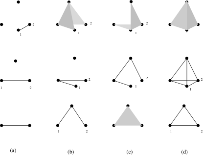
Figure 5: Bipartite entanglement among the qubits 1 and 2. (a) direct, (b) indirect, (c) configurations without entanglement, and (d) configurations that can result in cancellations of entanglement.

Trilinear terms correspond to surfaces and by the Eq. (29) we see that their presence in the canonical form of three qubits results in nonvanishing $3$-tangle, as in Fig. 6.(a). This is not the only configuration that permits tripartite entanglement; a loop consisting of three lines is also a configuration with genuine tripartite entanglement, as in Eq. (29). The inverse statement is not true for three qubits, since the term $\beta_{7}$ is not present in the expression of concurrence.

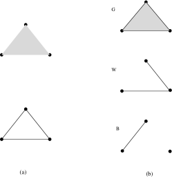
Figure 6: (a) Tripartite entanglement in two different configurations. (b) The three classes of entanglement for three qubits. $B$ stands for biseparable, $W$ for the singular class containing the Werner state and $G$ for the the general orbit.

As an application, in Fig. 6.(b) we represent the three classes of entanglement for three qubits diagrammatically way. It is important to note that if a diagrams is connected, i.e., there is a closed loop or surface, then this property cannot change under general local transformations.

We anticipate that the diagrammatic technique can be generalized to more qubits and improved with directed lines, surfaces and volumes that would aid in visualizing of cancellations or joint contributions. It appears that $N$-partite entanglement can be attributed not only to the coefficients in front of the $N$-th order monomials, but also to products of lower-order coefficients.

b.  Summarizing entanglement classes under $SL(2,\mathbb{C})$ transformations In Sect. III.D.4, we have shown how do the $sl$-entanglement classes emerge from the consideration of the tanglemeter dynamics under controlled action of continuous local transformations when proper feedback requirements are imposed. The general class has been identified along with four different singular classes, corresponding to one, two, three, and four vanishing eigenvectors of the determinant (69). All these classes were characterized by three complex parameters. Here, we further refine this analysis and add some singular classes that depend on less parameters in order to compare this classification with that given in Ref. Verstraete . We illustrate the correspondence, when normalize the states of Ref. Verstraete to unit vacuum amplitude and compare these states with ones suggested by $sl$-tanglemeters.

Let us remind that the $sl$-tanglemeter for four qubits we obtain in two steps. We first employ eight out of twelve complex parameters of local $SL$ transformations and put the generic state depending initially on fifteen complex parameters to the form of Eq. (27), which depends only on seven complex parameters. Then we chose the rest of the available transformations, four scaling operators $e^{B_{i}\sigma_{i}^{z}}$, in order to reduce the $sl$-tanglemeter to the form of Eq. (28). However, the second step not always possible to perform: when the tanglemeter is singular and one or more of the coefficients $\beta$ equal zero, the scalings can simplify the nilpotential further, although not to the form of Eq.  (28). For example, when in Eq. (27) $\beta_{3}=0$, the tanglemeter can be set in the form

$$f_{C} =\sigma_{3}^{+}\sigma_{4}^{+}+\beta_{5}(\sigma_{1}^{+}\sigma_{3}^{+}+\sigma_{2}^{+}\sigma_{4}^{+})$$

$$+\beta_{6}(\sigma_{1}^{+}\sigma_{4}^{+}+\sigma_{2}^{+}\sigma_{3}^{+})+\sigma_{1}^{+}\sigma_{2}^{+}\sigma_{3}^{+}\sigma_{4}^{+}~{},$$

characterized by only two parameters. For $\beta_{3}=\beta_{10}=0$ it reads

$$f_{C}=\sigma_{3}^{+}\sigma_{4}^{+}+\sigma_{1}^{+}\sigma_{3}^{+}+\beta_{6}(\sigma_{1}^{+}\sigma_{4}^{+}+\sigma_{2}^{+}\sigma_{3}^{+})+\sigma_{1}^{+}\sigma_{2}^{+}\sigma_{3}^{+}\sigma_{4}^{+}~{},$$

and $\beta_{3}=\beta_{10}=\beta_{9}=0$ results in

$$f_{C}=\sigma_{3}^{+}\sigma_{4}^{+}+\sigma_{1}^{+}\sigma_{3}^{+}+\sigma_{2}^{+}\sigma_{3}^{+}+\sigma_{1}^{+}\sigma_{2}^{+}\sigma_{3}^{+}\sigma_{4}^{+}~{}.$$

When the four-linear coefficient $\beta_{15}=0$ and one or more of the quadratic coefficients are also zero, the singular classes of states without fourpartite entanglement emerge: the $sl$-tanglemeter of four-qubit $W$ state

$$f_{C}=\sigma_{3}^{+}\sigma_{4}^{+}+\sigma_{1}^{+}\sigma_{3}^{+}+\sigma_{2}^{+}\sigma_{3}^{+},$$

belongs to one of these classes, and separable states with tanglemeters of the type

$$f_{C}=\sigma_{3}^{+}\sigma_{4}^{+}+\sigma_{2}^{+}\sigma_{3}^{+}+\sigma_{2}^{+}\sigma_{4}^{+}~{},$$

and similar, belong to other.

Consider now several special cases of the singular class Eq. (75), where all four of the eigenvalues of the determinant (69) are zero. When, in addition, one or several of the trilinear coefficients equal zero, it becomes possible to rescale one or more of the bilinear coefficients to unity. Less general classes with $sl$-tanglemeters like

$$f_{C} =\sigma_{1}^{+}\sigma_{3}^{+}\sigma_{4}^{+}+\sigma_{1}^{+}\sigma_{2}^{+}\sigma_{4}^{+}+\sigma_{2}^{+}\sigma_{3}^{+}\sigma_{4}^{+}+\sigma_{1}^{+}\sigma_{2}^{+}$$

$$+\beta_{5}\sigma_{1}^{+}\sigma_{3}^{+}+\beta_{6}\sigma_{2}^{+}\sigma_{3}^{+}~{},$$

$$f_{C} =\sigma_{1}^{+}\sigma_{2}^{+}\sigma_{4}^{+}+\sigma_{2}^{+}\sigma_{3}^{+}\sigma_{4}^{+}+\sigma_{1}^{+}\sigma_{2}^{+}+\sigma_{1}^{+}\sigma_{3}^{+}+\beta_{6}\sigma_{2}^{+}\sigma_{3}^{+}~{},$$

$$f_{C} =\sigma_{2}^{+}\sigma_{3}^{+}\sigma_{4}^{+}+\sigma_{1}^{+}\sigma_{2}^{+}+\sigma_{1}^{+}\sigma_{3}^{+}+\sigma_{2}^{+}\sigma_{3}^{+}$$

emerge as a result. One reveals more singular classes, when besides of several zero cubic coefficients, two or more quadratic terms vanish. Two examples

$$f_{C} =\sigma_{1}^{+}\sigma_{3}^{+}\sigma_{4}^{+}+\sigma_{1}^{+}\sigma_{2}^{+}\sigma_{4}^{+}+\sigma_{2}^{+}\sigma_{3}^{+}\sigma_{4}^{+}~{},$$

$$f_{C} =\sigma_{1}^{+}\sigma_{3}^{+}\sigma_{4}^{+}+\sigma_{1}^{+}\sigma_{2}^{+}\sigma_{4}^{+}+\sigma_{2}^{+}\sigma_{3}^{+}~{},$$

illustrate this case.

Different four-qubit classes emerging from this classification are presented in Table 1 along with the results of Ref. Verstraete . We include the general and main singular classes and omit a number of separable singular classes corresponding to product states. For the classes not symmetric under cyclic permutation of qubit indexes, this permutations is implicit. We note that our classes result from consideration of dynamic evolution that implies a series of sequential infinitesimal local operations preserving $su$-canonic form of the nilpotential. Therefore the situation, where some of the obtained classes turn out to be equivalent under a finite local $sl$-transformation, yet cannot be excluded with certainty. Keeping this in mind, it is easy to see that $G_{a}$ is identical to $G_{abcd}$ class that is also suggested in Ref. Akimasa . The class $L_{abc_{2}}$ corresponds to $LG2_{a}$, while $L_{a_{2}b_{2}}$ coincides with $LG1_{a}$. After applying $SL$ transformations on qubits 3 and 4 of the $L_{ab_{3}}$ class, the latter reduces to a form that is a singular case of the general class. The state $L_{a_{4}}$ can be set in the canonic form by flipping the second and third qubit, and then it is a special case of $G_{c}$ for $\beta_{6}=0$ and $\beta_{7}=i$. Continuing, $L_{a_{2}0_{3\oplus\bar{3}}}$ coincides with $S_{f}$, $L_{0_{7\oplus\bar{1}}}$ with $S_{b}$, and $L_{0_{3\oplus\bar{1}}0_{3\oplus\bar{1}}}$ with $S_{d}$. The singular class $L_{0_{5\oplus\bar{3}}}$ is of the $S_{a}$ form. Thus, we can conclude that the two classifications do overlap and complement each other.

General class	3 complex parameters
$G_{a}$	$f=\beta_{3}(\sigma_{1}^{+}\sigma_{2}^{+}+\sigma_{3}^{+}\sigma_{4}^{+})+\beta_{5}(\sigma_{1}^{+}\sigma_{3}^{+}+\sigma_{2}^{+}\sigma_{4}^{+})$
	$+\beta_{6}(\sigma_{1}^{+}\sigma_{4}^{+}+\sigma_{2}^{+}\sigma_{3}^{+})+\sigma_{1}^{+}\sigma_{2}^{+}\sigma_{3}^{+}\sigma_{4}^{+}$
Singular $3D$ classes	3 complex parameters
$G_{b}$	$f=\beta_{3}\left(\sigma_{1}^{+}\sigma_{2}^{+}+\sigma_{3}^{+}\sigma_{4}^{+}\right)+\beta_{5}\left(\sigma_{1}^{+}\sigma_{3}^{+}+\sigma_{2}^{+}\sigma_{4}^{+}\right)+\beta_{6}\left(\sigma_{1}^{+}\sigma_{4}^{+}+\sigma_{2}^{+}\sigma_{3}^{+}\right)$
	$+\sigma_{1}^{+}\sigma_{2}^{+}\sigma_{3}^{+}-\sigma_{1}^{+}\sigma_{2}^{+}\sigma_{4}^{+}+\sigma_{1}^{+}\sigma_{3}^{+}\sigma_{4}^{+}-\sigma_{2}^{+}\sigma_{3}^{+}\sigma_{4}^{+}$
	$+2\left(\beta_{5}\beta_{6}-\beta_{3}\beta_{6}+\beta_{3}\beta_{5}\right)\sigma_{1}^{+}\sigma_{2}^{+}\sigma_{3}^{+}\sigma_{4}^{+}$
$G_{c}$	$f=\sigma_{1}^{+}\sigma_{2}^{+}+\sigma_{1}^{+}\sigma_{3}^{+}+\sigma_{2}^{+}\sigma_{4}^{+}+\sigma_{3}^{+}\sigma_{4}^{+}+\beta_{6}\left(\sigma_{1}^{+}\sigma_{4}^{+}+\sigma_{2}^{+}\sigma_{3}^{+}\right)$
	$+\beta_{7}\left(\sigma_{1}^{+}\sigma_{2}^{+}\sigma_{3}^{+}-\sigma_{2}^{+}\sigma_{3}^{+}\sigma_{4}^{+}\right)+\beta_{11}\left(\sigma_{1}^{+}\sigma_{2}^{+}\sigma_{4}^{+}-\sigma_{1}^{+}\sigma_{3}^{+}\sigma_{4}^{+}\right)$
	$+2\sigma_{1}^{+}\sigma_{2}^{+}\sigma_{3}^{+}\sigma_{4}^{+}$
$G_{d}$	$f=\sigma_{1}^{+}\sigma_{2}^{+}+\sigma_{1}^{+}\sigma_{3}^{+}+\sigma_{2}^{+}\sigma_{4}^{+}+\sigma_{3}^{+}\sigma_{4}^{+}+\sigma_{1}^{+}\sigma_{4}^{+}+\sigma_{2}^{+}\sigma_{3}^{+}$
	$+\beta_{14}\left(\sigma_{1}^{+}\sigma_{2}^{+}\sigma_{3}^{+}-\sigma_{1}^{+}\sigma_{2}^{+}\sigma_{4}^{+}+\sigma_{1}^{+}\sigma_{3}^{+}\sigma_{4}^{+}-\sigma_{2}^{+}\sigma_{3}^{+}\sigma_{4}^{+}\right)$
	$+\beta_{13}\left(\sigma_{1}^{+}\sigma_{2}^{+}\sigma_{3}^{+}+\sigma_{1}^{+}\sigma_{2}^{+}\sigma_{4}^{+}-\sigma_{1}^{+}\sigma_{3}^{+}\sigma_{4}^{+}-\sigma_{2}^{+}\sigma_{3}^{+}\sigma_{4}^{+}\right)$
	$+\beta_{11}\left(\sigma_{1}^{+}\sigma_{2}^{+}\sigma_{3}^{+}-\sigma_{1}^{+}\sigma_{2}^{+}\sigma_{4}^{+}-\sigma_{1}^{+}\sigma_{3}^{+}\sigma_{4}^{+}+\sigma_{2}^{+}\sigma_{3}^{+}\sigma_{4}^{+}\right)$
	$+2\sigma_{1}^{+}\sigma_{2}^{+}\sigma_{3}^{+}\sigma_{4}^{+}$
$G_{e}$	$f=\sigma_{1}^{+}\sigma_{2}^{+}\sigma_{3}^{+}+\sigma_{1}^{+}\sigma_{2}^{+}\sigma_{4}^{+}+\sigma_{1}^{+}\sigma_{3}^{+}\sigma_{4}^{+}+\sigma_{2}^{+}\sigma_{3}^{+}\sigma_{4}^{+}+$
	$\beta_{3}\sigma_{1}^{+}\sigma_{2}^{+}+\beta_{6}\sigma_{2}^{+}\sigma_{3}^{+}+\beta_{5}\sigma_{2}^{+}\sigma_{3}^{+}$
Singular $2D$ classes	2 complex parameters
$LG2_{a}$	$f=\sigma_{3}^{+}\sigma_{4}^{+}+\beta_{5}(\sigma_{1}^{+}\sigma_{3}^{+}+\sigma_{2}^{+}\sigma_{4}^{+})+\beta_{6}(\sigma_{1}^{+}\sigma_{4}^{+}+\sigma_{2}^{+}\sigma_{3}^{+})+\sigma_{1}^{+}\sigma_{2}^{+}\sigma_{3}^{+}\sigma_{4}^{+}$
$LG2_{b}$	$f=\sigma_{1}^{+}\sigma_{2}^{+}+\sigma_{3}^{+}\sigma_{4}^{+}+\beta_{5}(\sigma_{1}^{+}\sigma_{3}^{+}+\sigma_{2}^{+}\sigma_{4}^{+})+\beta_{6}(\sigma_{1}^{+}\sigma_{4}^{+}+\sigma_{2}^{+}\sigma_{3}^{+})$
$LG2_{c}$	$f=\sigma_{1}^{+}\sigma_{3}^{+}\sigma_{4}^{+}+\sigma_{1}^{+}\sigma_{2}^{+}\sigma_{4}^{+}+\sigma_{2}^{+}\sigma_{3}^{+}\sigma_{4}^{+}+\sigma_{1}^{+}\sigma_{2}^{+}+\beta_{5}\sigma_{1}^{+}\sigma_{3}^{+}+\beta_{6}\sigma_{2}^{+}\sigma_{3}^{+}$
Singular $1D$ classes	1 complex parameters
$LG1_{a}$	$f=\sigma_{1}^{+}\sigma_{2}^{+}+\sigma_{1}^{+}\sigma_{3}^{+}+\beta_{6}(\sigma_{1}^{+}\sigma_{4}^{+}+\sigma_{2}^{+}\sigma_{3}^{+})+\sigma_{1}^{+}\sigma_{2}^{+}\sigma_{3}^{+}\sigma_{4}$
$LG1_{b}$	$f=\sigma_{1}^{+}\sigma_{2}^{+}\sigma_{4}^{+}+\sigma_{2}^{+}\sigma_{3}^{+}\sigma_{4}^{+}+\sigma_{1}^{+}\sigma_{2}^{+}+\sigma_{1}^{+}\sigma_{3}^{+}+\beta_{6}\sigma_{2}^{+}\sigma_{3}^{+}$
Singular point classes	no parameters
$S_{a}$	$f=\sigma_{1}^{+}\sigma_{2}^{+}\sigma_{3}^{+}+\sigma_{1}^{+}\sigma_{3}^{+}\sigma_{4}^{+}+\sigma_{2}^{+}\sigma_{4}^{+}$
$S_{b}$	$f=\sigma_{1}^{+}\sigma_{2}^{+}\sigma_{3}^{+}+\sigma_{1}^{+}\sigma_{3}^{+}\sigma_{4}^{+}+\sigma_{1}^{+}\sigma_{2}^{+}\sigma_{4}^{+}$
$S_{c}$	$f=\sigma_{1}^{+}\sigma_{2}^{+}\sigma_{3}^{+}+\sigma_{1}^{+}\sigma_{3}^{+}\sigma_{4}^{+}$
$S_{d}$	$f=\sigma_{1}^{+}\sigma_{2}^{+}\sigma_{3}^{+}$
$S_{e}$	$f=\sigma_{3}^{+}\sigma_{4}^{+}+\sigma_{1}^{+}\sigma_{3}^{+}+\sigma_{2}^{+}\sigma_{3}^{+}+\sigma_{1}^{+}\sigma_{2}^{+}\sigma_{3}^{+}\sigma_{4}^{+}$
$S_{f}$	$f=\sigma_{1}^{+}\sigma_{2}^{+}+\sigma_{2}^{+}\sigma_{3}^{+}+\sigma_{3}^{+}\sigma_{1}^{+}+\sigma_{1}^{+}\sigma_{2}^{+}\sigma_{3}^{+}\sigma_{4}^{+}$
$\dots$	$\dots$

Table 1: Classification of four-qubit entanglement classes following from $SL(2,\mathbb{C})$ transformation properties of the canonic form.

VI.3 Equation for local and two-body interaction

We give here some more details on the derivation of the dynamic equation for the nilpotential $f$. Consider a single gate operation applied to qubits $i$ and $j$. We cast the function $f$ in the form $f_{00}+\sigma_{i}^{+}f_{01}+\sigma_{j}^{+}f_{10}+\sigma_{i}^{+}\sigma_{j}^{+}f_{11}$, and find

$$\mathrm{e}^{-f} =\mathrm{e}^{-f_{00}}\left[1-\sigma_{i}^{+}f_{01}-\sigma_{j}^{+}f_{10}-\sigma_{i}^{+}\sigma_{j}^{+}(f_{11}-f_{01}f_{10})\right]$$

$$\mathrm{e}^{f} =\mathrm{e}^{f_{00}}\left[1+\sigma_{i}^{+}f_{01}+\sigma_{j}^{+}f_{10}+\sigma_{i}^{+}\sigma_{j}^{+}(f_{11}+f_{01}f_{10})\right]~{},$$ (132)

where the coefficients

$$f_{00} =f-\sigma_{i}^{+}\frac{\partial f}{\partial\sigma_{i}^{+}}-\sigma_{j}^{+}\frac{\partial f}{\partial\sigma_{j}^{+}}+\sigma_{i}^{+}\sigma_{j}^{+}\frac{\partial^{2}f}{\partial\sigma_{i}^{+}\partial\sigma_{j}^{+}}\,,$$

$$f_{01} =\frac{\partial f}{\partial\sigma_{i}^{+}}-\sigma_{j}^{+}\frac{\partial^{2}f}{\partial\sigma_{i}^{+}\partial\sigma_{j}^{+}}\,,\hskip 14.22636ptf_{10}=\frac{\partial f}{\partial\sigma_{j}^{+}}-\sigma_{i}^{+}\frac{\partial^{2}f}{\partial\sigma_{i}^{+}\partial\sigma_{j}^{+}}\,,\hskip 14.22636ptf_{11}=\frac{\partial^{2}f}{\partial\sigma_{i}^{+}\partial\sigma_{j}^{+}}\,,$$ (133)

are independent of $\sigma_{i}^{+},\sigma_{j}^{+}$. Upon substituting these equations into Eq. (50) for the Hamiltonian in Eq. (58), bearing in mind Eq. (54), we obtain

$$\mathrm{i}\frac{\partial f}{\partial t} =P_{i}^{-}\sigma_{i}^{+}+P_{j}^{-}\sigma_{j}^{+}+P_{i}^{+}\frac{\partial f}{\partial\sigma_{i}^{+}}+P_{j}^{+}\frac{\partial f}{\partial\sigma_{j}^{+}}-P_{i}^{+}\sigma_{i}^{+}\left(\frac{\partial f}{\partial\sigma_{i}^{+}}\right)^{2}-P_{j}^{+}\sigma_{j}^{+}\left(\frac{\partial f}{\partial\sigma_{j}^{+}}\right)^{2}$$

$$+G_{ij}\bigg{[}\sigma_{j}^{+}\frac{\partial f}{\partial\sigma_{i}^{+}}+\sigma_{i}^{+}\frac{\partial f}{\partial\sigma_{j}^{+}}-\sigma_{i}^{+}\sigma_{j}^{+}\left(\frac{\partial f}{\partial\sigma_{i}^{+}}\right)^{2}-\sigma_{i}^{+}\sigma_{j}^{+}\left(\frac{\partial f}{\partial\sigma_{j}^{+}}\right)^{2}\bigg{]}\>.$$ (134)

Summing over $i,j$ yields Eq. (59), where the condition $G_{ij}=G_{ji}$ is taken into account.

VI.4 Derivation of $3$-tangle based on the tanglemeter

Here we present a derivation of $3$-tangle that is based directly on the transformations of amplitudes under local operations. The explicit expression for $3$-tangle has the rather simple form of Eq. (30), when written for the $su$-canonical state. When considering $SL$ transformations, we look for a quantity that takes different values within the generic $sl$ orbit of three qubits, and vanishes outside this orbit. Performing $SL$-transformations, we can still set appropriate conditions so as to preserve the $su$-canonical form of states.

We start with the $sl$-canonical state, i.e., is the maximum entangled state
$\left(\left|000\right\rangle+\left|111\right\rangle\right)/\sqrt{2}$, written in terms of nilpotent variables and normalizing to unit reference state amplitude:

$$|\psi\rangle=\frac{1}{\sqrt{2}}(1+\sigma_{1}^{+}\sigma_{2}^{+}\sigma_{3}^{+})|000\rangle~{}~{}.$$

Then we apply to each qubit the general $SL(2,\mathbb{C})$ transformation, which reads

$$e^{A_{i}\sigma_{i}^{-}}e^{B_{i}\sigma_{i}^{z}}e^{C_{i}\sigma_{i}^{+}},~{}~{}A_{i},B_{i},C_{i}\in{\mathbb{C}},\,i=1,2,3.$$

This transformation results in the most general admissible $su$-canonical form of the $su$-canonical state,

$$|\psi^{\prime}\rangle =(\psi_{000}^{\prime}+\psi_{011}^{\prime}\sigma_{1}^{+}\sigma_{2}^{+}+\psi_{110}^{\prime}\sigma_{2}^{+}\sigma_{3}^{+}$$

$$+\psi_{101}^{\prime}\sigma_{1}^{+}\sigma_{3}^{+}+\psi_{111}^{\prime}\sigma_{1}^{+}\sigma_{2}^{+}\sigma_{3}^{+})|000\rangle~{},$$

in which the coefficients take the forms

$$\psi_{000}^{\prime} =\frac{(1+z)^{2}}{\sqrt{2}}\mathrm{e}^{-B_{1}-B_{2}-B_{3}},$$ (135)

$$\psi_{011}^{\prime} =-\frac{1+z}{z\sqrt{2}}C_{1}C_{2}\mathrm{e}^{B_{1}+B_{2}-B_{3}}$$

$$\psi_{101}^{\prime} =-\frac{1+z}{z\sqrt{2}}C_{1}C_{3}\mathrm{e}^{B_{1}+B_{3}-B_{2}}$$

$$\psi_{110}^{\prime} =-\frac{1+z}{z\sqrt{2}}C_{2}C_{3}\mathrm{e}^{B_{2}+B_{3}-B_{1}}$$

$$\psi_{111}^{\prime} =-\frac{1+2z}{z^{2}\sqrt{2}}C_{1}C_{2}C_{3}\mathrm{e}^{B_{1}+B_{2}+B_{3}}~{}~{}.$$

Here we have employed a complex variable $z$ that naturally emerges from the requirements of $su$-canonical form, having the relations $z=A_{1}e^{2B_{1}}C_{1}=A_{2}e^{2B_{2}}C_{2}=A_{3}e^{2B_{3}}C_{3}$ and $(1+z)^{2}C_{2}C_{3}=-z^{2}$. One sees that the amplitudes of the $su$-canonical state depend on seven real parameters, since in addition to five parameters of the tanglemeter, we now allow for two more parameters characterizing the vacuum state amplitude.

Being in the general orbit, states of less general orbits can be reached if irreversible transformations are performed Akimasa corresponding to the limit $|z|\rightarrow\infty$. At this point we want to construct a polynomial measure on the amplitudes $\psi^{\prime}$, such a way that it is a function of $z$ and it vanishes outside the general $sl$-orbit. Direct inspection shows that we can construct a function that depends only on the parameter $z$

$$\zeta(z)=\frac{\psi_{111}^{{}^{\prime}2}\psi_{000}^{{}^{\prime}2}}{\psi_{000}^{\prime}\psi_{110}^{\prime}\psi_{011}^{\prime}\psi_{101}^{\prime}}=-\frac{(1+2z)^{2}}{z(1+z)}~{},$$ (136)

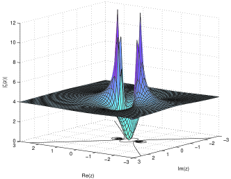
Figure 7: Function $|\zeta(z)|$ as in Eq. (136). In the limit $|z|\rightarrow\infty$, $|\zeta(z)|\rightarrow 4$.

and is independent of the normalization,. The function $\zeta(z)$ shown in Fig. 7 can take any value, but $-4$ that corresponds to the limit $|z|\rightarrow\infty$. Therefore, the polynomial

$$\left|\psi_{111}^{{}^{\prime}2}\psi_{000}^{{}^{\prime}2}+4\psi_{000}^{\prime}\psi_{110}^{\prime}\psi_{011}^{\prime}\psi_{101}^{\prime}\right|$$

will be identically zero outside the general orbit, and is otherwise nothing but the $3$-tangle expressed in terms of the coefficients of the canonical nilpotent polynomial, Eq. (30).

This procedure for constructing a measure can be in principle extended to more qubits. However, the extension will require some care. The general $sl$-orbit of four qubits is characterized by six parameters parameters, in contrast to the three-qubits case. Consequently, irreversible transformations may connect different $sl$-orbits that both contain $N$-partite entanglement. Therefore the desired limits need to be clearly specified.

Finally, we would like to mention that Theorem 3 in Ref. Verstraete2 suggests another useful application of the $\zeta(z)$ function. For an arbitrary $3$-qubit state expressed in canonical form, one can calculate the value of $\zeta(z)$ by direct substitution of the numerical values of amplitudes to Eq. (136), and then solve a binomial equation to find the root $z=z_{r}$. One can choose the coefficients $A_{i},~{}B_{i}$, and $C_{i}$ such that they satisfy $A_{i}\mathrm{e}^{2B_{i}}C_{i}=z_{r}$. In this way a determinant-$1$ transformation that brings the maximum entangled state to the chosen state can be identified explicitly. The inverse transformation can be used for an optimal filtering procedure called purification, a probabilistic procedure that transforms a state of the general orbit to the one with the maximal entanglement,i.e. to the $GHZ$ state.

References

- (1) A. Einstein, B. Podolsky, and N. Rosen, Phys. Rev. 47, 777 (1935).
- (2) E. Schrödinger, Proc. Cambridge Phylosoph. Soc. 31, 555 (1935).
- (3) M. A. Nielsen and I. L. Chuang, Quantum Computation and Information (Cambridge University Press, Cambridge, England, 2000).
- (4) C. H. Bennett, G. Brassard, C. Crépeau, R. Jozsa, A. Peres, and W. K. Wootters, Phys. Rev. Lett. 70, 1895 (1993); S.L. Braunstein, G.M. D’Ariano, G.J. Milburn, and M.F. Sacchi, Phys. Rev. Lett. 84, 3486 (2000).
- (5) A. Ekert, Phys. Rev. Lett. 67, 661 (1991); J. Kempe, Phys. Rev. A 60, 910 (1999).
- (6) R. Jozsa and N. Linden, Proc. R. Soc. London A 459, 2001 (2003).
- (7) R. Orus and J. I. Latorre, Phys. Rev. A 69, 052308 (2004).
- (8) A. Tal and G. Kurizki, Phys. Rev. Lett. 94, 160503 (2005); T. Opatrny, B. Deb, and G. Kurizki, Phys. Rev. Lett. 90, 250404 (2003).
- (9) B. Georgeot and D. L. Shepelyansky, Phys. Rev. E 62, 3504 (2000); S. Bettelli and D. L. Shepelyansky, Phys. Rev. A 69, 054303 (2003).
- (10) C. Mejia-Monasterio, G. Benenti, G. G. Carlo, and G. Casati, Phys. Rev. A 71, 062324 (2005).
- (11) L. F. Santos, G. Rigolin, and C. O. Escobar, Phys. Rev. A 69, 042304 (2004).
- (12) S. Montangero, G. Benenti, and R. Fazio, Phys. Rev. Lett. 91, 187901 (2003); S. Montangero and L. Viola, quant-ph/0507099.
- (13) M. C. Arnesen, S. Bose, and V. Vedral, Phys. Rev. Lett. 87, 017901 (2001).
- (14) T. J. Osborne and M. A. Nielsen, Phys. Rev. A 66, 032110 (2002).
- (15) G. Vidal, J. I. Latorre, E. Rico, and A. Kitaev, Phys. Rev. Lett. 90, 227902 (2003).
- (16) R. Eryigit, R. Eryigit, and Y. Gunduc, - model, Int. J. Mod. Phys. C 15, 1095 (2004).
- (17) P. Stelmachovi and V. Buzek, Phys. Rev. A 70, 032313 (2004).
- (18) L. Amico, A. Osterloh, F. Plastina, R. Fazio, and G. M. Palma, Phys. Rev. A 69, 022304 (2004).
- (19) R. Somma, G. Ortiz, H. Barnum, E. Knill, and L. Viola, Phys. Rev. A 70, 042311 (2004).
- (20) T.-C. Wei, D. Das, S. Mukhopadyay, S. Vishveshwara, and P. M. Goldbart, Phys. Rev. A 71, 060305(R) (2005).
- (21) T. S. Cubitt, F. Verstraete, and J. I. Cirac, Phys. Rev. A 71, 052308 (2005).
- (22) D.M. Greeberger, M. Horne, A. Shimony, and A. Zeilinger, Am. J. Phys. 58, 1131 (1990).
- (23) W. Dur, G. Vidal, and J. I. Cirac, Phys. Rev. A. 62, 062314 (2000).
- (24) F. Verstraete, J. Dehaene, B. DeMoor, and H. Verschelde, Phys. Rev. A 65, 052112 (2002).
- (25) A. Peres, Phys. Rev. Lett. 77, 1413 (1996).
- (26) W. K. Wootters, Phys. Rev. Lett. 80, 2245 (1998); V. Coffman, J. Kundu and W. K. Wooters, 052306 (2000).
- (27) V. Vedral, M. P. Plenio, M. A. Rippin, and P. L. Knight, Phys. Rev. Lett. 78, 2275 (1997).
- (28) D. A. Meyer and N. R. Wallach, J. Math. Phys. 43, 4273 (2002).
- (29) A. Wong and N. Christensen, Phys. Rev. A, 63, 044301 (2001).
- (30) P. Rungta, V. Buzek, C. M. Caves, M. Hillery, and G. J. Milburn, Phys. Rev. A 64, 042315 (2001).
- (31) C. H. Bennett, S. Popescu, D. Rohrlich, J. A. Smolin, and A. V. Thapliyal, Phys. Rev. A 63, 012307 (2001).
- (32) H. Heydari and G. Björk, J. Phys. A 37, 9251 (2004).
- (33) F. Verstraete, J. Dehaene, and B. De Moor, Phys. Rev. A 68, 012103 (2003).
- (34) A. Acin, A. Andrianov, L. Costa, E. Jane, J. I. Latorre, and R. Tarrach, Phys. Rev. Lett. 85, 1560 (2000); A. Acin, A. Andrianov, E. Jane, J. I. Latorre, and R. Tarrach, J. Phys. A 34, 6725 (2001).
- (35) A. Miyake, Phys. Rev. A 67, 012108 (2003); A. Miyake, F. Verstraete, Phys. Rev. A 69, 012101 (2004).
- (36) M. Grassl, M. Rötteler, and T. Beth, Phys. Rev. A 58, 1833 (1998).
- (37) H. Barnum and N. Linden, J. Phys. A 34, 6787 (2001).
- (38) M. S. Leifer, N. Linden, and A. Winter, Phys. Rev. A 69, 052304 (2004).
- (39) R. M. Gingrich, Phys. Rev. A 65, 052302 (2002).
- (40) A. Osterloh and J. Siewert, quant-ph/0410102.
- (41) J. G. Luque and J. Y. Thibon, Phys. Rev. A 67, 042303 (2003).
- (42) G. Vidal, J. Mod. Opt. 47, 355 (2000).
- (43) C. H. Bennett, H. J. Bernstein, S. Popescu, and B. Schumacher, Phys. Rev. A 53, 2046 (1996).
- (44) J.-G. Luque and J.-Y. Thibon, quant-ph/0506058.
- (45) H. A. Carteret, A. Higuchi, and A. Sudbery, J. Math. Phys., 41, 7932 (2000).
- (46) T. A. Brun and O. Cohen, Phys. Lett. A 281, 88 (2001).
- (47) A. Sudbery, J. Phys. A 34, 643 (2001); H. A. Carteret and A. Sudbery, J. Phys. A 33, 4981 (2000).
- (48) E. Briand, J.-G. Luque, and J.-Y. Thibon, J. Math. Phys. 43, 4855 (2004).
- (49) The available classification relies on the structure of Dynkin diagrams. This was kindly communicated to A. M. and V. A. by Victor Kaç.
- (50) N. Linden and S. Popescu, Fortschr. Phys. 46, 567 (1998).
- (51) J. K. Stockton, J. M. Geremia, A. C. Doherty and H. Mabuchi, Phys. Rev. A 67, 022112 (2003).
- (52) Capital letters and will normally denote Lie groups, while the small and denote the corresponding Lie algebras. However, we do not always follow this convention, unless it creates a confusion.
- (53) F. A. Berezin, The Method of Second Quantization (Academic Press, Cambridge, 1966).
- (54) K. Efetov, Supersymmetry in Disorder and Chaos (Cambridge University Press, Cambridge, 1997).
- (55) A. Barenco, C. H. Bennett, R. Cleve, D. P. DiVincenzo, N. Margolus, P. Shor, T. Sleator, J. Smolin, H. Weinfurter, Phys. Rev. A 52, 3457 (1995); S. Lloyd, Phys. Rev. Lett. 75, 346 (1995).
- (56) J. L. Cereceda, quant-ph/0305043.
- (57) L.-B. Fu, J.-L. Chen, and X.-G. Zhao, Phys. Rev. A 68, 022323 (2003).
- (58) H. Barnum, E. Knill, G. Ortiz, R. Somma, L. Viola, Phys. Rev. Lett. 92, 107902 (2004).
- (59) H. Barnum, E. Knill, G. Ortiz, and L. Viola, Phys. Rev. A 68, 032308 (2003).
- (60) S. L. Akhtarshenas, quant-ph/0311166.
- (61) Still there is a strong indication that the maximum population is unique. Indeed, there exists a unique local unitary operation which being applied to a single-qubit density matrices maximizes its ground state polpulation. Such transformations applied to all qubits maximize the assembly ground state population.
- (62) K. Vogel, V.M. Akulin, and W. P. Schleich, Phys. Rev. Lett. 71, 1816 (1993).
- (63) We therefore do not address the purification protocols.
- (64) D. M. Greenberger, M. Horne, and A. Zeilinger, in Bell’s Theorem, Quantum Theory, and Conceptions of the Universe, M. Kafatos Ed., (Kluwer, Dordrecht, 1989), pp.69-72.
- (65) Actually, a finite number of different canonic states may exist, that can be transformed one to another by -transformations consisting of qubit-“flips” and scaling. In order to be specific we can choose one which has minimum .
- (66) A mathematician would say that represents an invariant tensor of both and transformations. On the other hand, the tensor is invariant under , but not under .
- (67) This operation may also be defined as integration over the nilpotent variable, by the analogy to well-known anticommuting Grassman variables Berezin .
- (68) L. Viola, H. Barnum, E. Knill, G. Ortiz, and R. Somma, quant-ph/0403044, in: Coding Theory and Quantum Computing, AMS series in Contemporary Mathematics, Vol. 381, D. Evans et al Eds. (Americal Mathematical Society, Providence, Rhode Island, 2005), pp. 117–130; H. Barnum, G. Ortiz, R. Somma, and L. Viola, quant-ph/0506099.
- (69) J. F. Cornwell, Group Theory in Physics (Academic Press, San Diego, 1997).
- (70) J. E. Humphreys, Introduction to Lie Algebras and Representation Theory (Springer, New York, 1972).
- (71) We emphasize that we express the state vector via commuting root vectors and not via the so-called simple root vectors whose multiple commutators give all elements of the set (in the case of , the simple roots are and ).
- (72) A. M. Perelomov, Generalized Coherent States and their Applications (Springer, Berlin, 1986).
- (73) W.-M. Zhang, D. H. Feng, and R. Gilmore, Rev. Mod. Phys. 62, 867 (1990).
- (74) R. Glauber, Phys. Rev. 131, 2766–2788 (1963).
- (75) Note that, however, none of these algebras are semisimple or reductive, hence care must be taken in defining notions such as Cartan decomposition etc.
- (76) See Ref. Efetov for details.
- (77) V. M. Akulin, Coherent Dynamics of Complex Quantum Systems (Springer, 2005).
- (78) M. Takahashi, Thermodynamics of One-Dimensional Solvable Models (Cambridge University Press, Cambridge, 1999).