Approximations by graphs and emergence of global structures

Abstract

We study approximations of billiard systems by lattice graphs. It is demonstrated that under natural assumptions the graph wavefunctions approximate solutions of the Schrödinger equation with energy rescaled by the billiard dimension. As an example, we analyze a Sinai billiard with attached leads. The results illustrate emergence of global structures in large quantum graphs and offer interesting comparisons with patterns observed in complex networks of a different nature.

I Introduction

The notion of a quantum graph is known for more then half a century RuS , however, an intense investigation of these structures started less than two decades ago ARZ ; ES1 as a response to progress in fabrication technologies which allowed to prepare microscopic graph-like structures. Nowadays, there is an extensive literature devoted to the subject; for recent reviews see KS ; Ku and also AGHH .

An attention to quantum graphs come from the fact that motion on their edges is easy to describe, and at the same time the graph structure leads to a nontrivial behavior. It was shown, in particular, that even a graph with a small number of vertices is capable of developing an internal dynamics rich enough to display universality features that are typical for the wave-chaotic behavior BBK ; ks1 ; ks2 . It is not only a theory, the results can be checked experimentally in a microwave graph model sirko1 .

On the contrary, properties of nontrivial large-scale graphs have been regarded as less interesting due to the expected localization of the corresponding wavefunctions. An indication that this belief is wrong may be seen from the fact that complex graph-like structures, such as systems of interconnected neurons, display surprising patterns observed, for instance, in the visual cortex of mammals blasdel . It was shown in Geisel that these patterns can be understood as a manifestation of a Gaussian random field, and are in this sense analogous to patterns emerging in two dimensional quantum chaotic systems, for instance, nodal domains in a chaotic quantum billiard blum .

A thorough investigation of such structures on graphs is by no means easy. To follow the mentioned example, a nodal domain is a connected component of the maximal induced subgraph of a graph $\Gamma$ on which a function does not change sign; it relates the pattern formation on $\Gamma$ to nontrivial algebraic questions about graph partition, etc. This is probably the reason why only few mathematical results of this type are available at present - cf. biyi1 ; biyi2 .

In this paper we are going to show that extended graphs support structures similar to those known from two-dimensional wave chaos and Gaussian random-field models. We will show that the structures do not depend on the local set up of the graph. They reflect the influence of the graph boundary on the wave propagation and interference on the graph. The final patterns are ”global” in the sense that they extend over hundreds of graph vertices.

Our approach is based on graph embedding into a Euclidean space and a convergence argument; we will demonstrate that wavefunctions on the graph can approximate solutions of the respective “continuous” billiard problem. The embedding assumption is naturally a nontrivial restriction because not every graph can be regarded as a subset of a Euclidean space from which it inherits its metric. It applies, however, to wide enough class of systems and allows us at the same time to circumvent difficulties of a pure algebraic treatment.

The technical tool to derive the approximation result is a graph duality adopted from Ex1 . To make the paper self-contained we review this theory in the next section in a simplified form suitable for the present purpose. Then we will show how solutions to the Schrödinger equation can be approximated by those of a Schrödinger equation on lattice graphs with the energy properly rescaled.

To illustrate the result we will analyze an example of a lattice graph which approximates a Sinai billiard. Since we want to go beyond the nodal structure and to analyze also the phase behavior of the wavefunctions we will study such a also from the transport point of view, attaching to it a pair of semiinfinite leads; the result will be compared to the ”true” Sinai billiard with a pair of leads attached. We will compare, in particular, the probability currents and show they are similar to each other provided the current on the graph is properly defined as a vector sum of currents at the graphs links.

II Theory: a graph duality

By $\Gamma$ we denote in the following a connected graph consisting of at most countable families of vertices $\mathcal{V}=\{{\mathcal{X}}_{j}:\,j\in I\}$ and edges $\mathcal{L}=\{\mathcal{L}_{jn}:\,(j,n)\in I_{\mathcal{L}}\subset I\times I\}$. We suppose that each pair of vertices is connected by not more than one link, otherwise we can simply add vertices to any “multiple” edge. The set $\mathcal{N}(\mathcal{X}_{j})=\{\mathcal{X}_{n}:\,n\in\nu(j)\subset I\setminus\{j\}\}$ consists of the neighbors of $\mathcal{X}_{j}$, i.e. the vertices connected with $\mathcal{X}_{j}$ by a single edge is nonempty by assumption. The graph boundary $\mathcal{B}$ consists of vertices having a single neighbor; it may be empty. We denote by $I_{\mathcal{B}}$ and $I_{\mathcal{I}}$ the index subsets in $I$ corresponding to $\mathcal{B}$ and the graph interior $\mathcal{I}:=\mathcal{V}\setminus\mathcal{B}$, respectively.

We suppose that $\Gamma$ is a metric graph, i.e. that it has a local metric structure, every edge $\mathcal{L}_{jn}$ being isometric with a line segment $[0,\ell_{jn}]$. Of course, the graph can be also equipped with a global metric, for instance, by identifying it with a subset of $\mathbb{R}^{\nu}$. In general the metrics may not coincide, however, in the next section we will identify them. Using the local metric, we introduce the Hilbert space $L^{2}(\Gamma):=\bigoplus_{(j,n)\in I_{\mathcal{L}}}L^{2}(0,\ell_{jn})$ whose elements are $\psi=\{\psi_{jn}:\,(j,n)\in I_{\mathcal{L}}\}$ or simply $\{\psi_{jn}\}$; in the same way we define Sobolev spaces on $\Gamma$. Given a family of potentials $U:=\{U_{jn}\}$ with $V_{jn}\in L^{\infty}(0,\ell_{jn})$ and coupling constants $\alpha:=\{\alpha_{j}\in\mathbb{R}:\>j\in I\}$, we define the Schrödinger operator $H_{\alpha}\equiv H_{\alpha}(\Gamma,U)$ by

$$H_{\alpha}\{\psi_{jn}\}:=\{\,-\psi^{\prime\prime}_{jn}+U_{jn}\psi_{jn}:\;(j,n)\in I_{\mathcal{L}}\,\}$$ (2.1)

on the domain consisting of all $\psi$ with $\psi_{jn}\in W^{2,2}(0,\ell_{jn})$ satisfying suitable boundary conditions at the vertices linking the boundary values

$$\psi_{jn}(j):=\lim_{x\to 0+}\psi_{jn}(x)\,,\quad\psi^{\prime}_{jn}(j):=\lim_{x\to 0+}\psi^{\prime}_{jn}(x)\,,$$ (2.2)

where the point $x=0$ is identified with $\mathcal{X}_{j}$. Specifically, we will work here with the so-called $\delta$ coupling: at any $\mathcal{X}_{j}\in\mathcal{V}$ we have $\,\psi_{jn}(j)=\psi_{jm}(j)=:\psi_{j}$ for all $n,m\in\nu(j)$, and

$$\sum_{n\in\nu(j)}\psi^{\prime}_{jn}(j)=\alpha_{j}\psi_{j}\,;$$ (2.3)

it is known that among all (non-trivial) boundary conditions which make the operator (2.1) self-adjoint there are no other with wavefunctions continuous at the vertices ES1 . The particular case $\alpha=0$ represents the most simple boundary conditions, called usually Kirchhoff KS , which we will employ in the example of Sec. IV, however, for the moment it is useful to consider the more general situation (2.3). Furthermore, if the boundary $\mathcal{B}\neq\emptyset$ we assume Dirichlet boundary conditions there,

$$\psi_{j}=0\,,\quad j\in I_{\mathcal{B}}\,.$$ (2.4)

If $\Gamma$ is infinite one can look not only for bound states of $H_{\alpha}$ but also for solutions of the equation

$$H_{\alpha}\psi=k^{2}\psi$$ (2.5)

referring to the continuous spectrum. To describe the generalized eigenfunctions we consider in such a case the class $D_{\rm loc}(H_{\alpha})$ which is the subset in $\bigvee_{(j,n)\in I_{\mathcal{L}}}L^{2}(0,\ell_{jn})\,$ (the direct sum) consisting of the functions which satisfy all the requirements imposed at $\psi\in D(H_{\alpha})$ except the global square integrability. The conditions (2.3) define self-adjoint operators also if the $\alpha_{j}$’s are formally put equal to infinity. We exclude this possibility, which corresponds to Dirichlet decoupling of the operator at $\mathcal{X}_{j}$ turning the vertex effectively into $N_{j}$ points of the boundary.

We need the decoupling, however, to state the result. Let $H_{\alpha}^{D}$ be the operators obtained from $H_{\alpha}$ by changing the conditions (2.3) at the points of $\mathcal{I}$ to Dirichlet and denote $\mathcal{K}:=\{k:\,k^{2}\in\sigma(H_{\alpha}^{D})\}$. In the particular case when the particle is free at graph edges, $U_{jn}=0$, this set is given explicitly as $\mathcal{K}:=\{\pi n\ell_{jn}^{-1}:\,(j,n)\in\mathcal{I}_{\mathcal{L}},\,n\in\mathbb{N}_{+}\}$. We will adopt several assumptions, namely

(i)  all the potentials of the family $\{U_{jn}\}$ are uniformly bounded for $(j,n)\in I_{\mathcal{L}}\,$,

(ii) $\ell_{0}:=\inf\{\,\ell_{jn}:\,(j,n)\in I_{\mathcal{L}}\}>0\,$,

(iii) $L_{0}:=\sup\{\,\ell_{jn}:\,(j,n)\in I_{\mathcal{L}}\}<\infty\,$,

(iv) $\;N_{0}:=\max\{\,\#\nu(j):\,j\in I\,\}<\infty\,$.

To formulate the result, we need a few more notions. On $\mathcal{L}_{nj}\equiv[0,\ell_{jn}]$, where the right endpoint identified with the vertex $\mathcal{X}_{j}$, we denote as $u_{jn}$ and $v_{jn}$ the solution to $-f^{\prime\prime}+U_{jn}f=k^{2}f$ which satisfy the normalized Dirichlet boundary conditions

$$u_{jn}(\ell_{jn})=1\!-\!(u_{jn})^{\prime}(\ell_{jn})=0\,,\;\;v_{jn}(0)=1\!-\!(v_{jn})^{\prime}(0)=0\,;$$

their Wronskian is naturally equal to $W_{jn}=-v_{jn}(\ell_{jn})=u_{jn}(0)$. After this preliminary we can specify the result of Ex1 to the present situation.
Theorem: (a) Let assumptions (i)–(iv) be satisfied and suppose that $\psi\in D_{loc}(H_{\alpha})$ solves (2.5) for some $k\not\in\mathcal{K}_{\alpha}$ with $k^{2}\in\mathbb{R}$, $\mathrm{Im\,}k\geq 0$. Then the corresponding boundary values (2.2) satisfy the equation

$$\sum_{n\in\nu(j)\cap I_{\mathcal{I}}}{\psi_{n}\over W_{jn}}\,-\,\left(\,\sum_{n\in\nu(j)}{(v_{jn})^{\prime}(\ell_{jn})\over W_{jn}}-\alpha_{j}\,\right)\psi_{j}\,=\,0\,.$$ (2.6)

Conversely, any solution $\{\psi_{j}:\,j\in I_{\mathcal{I}}\}$ of the system to (2.6) determines a solution of (2.5) by

$$\psi_{jn}(x)={\psi_{n}\over W_{jn}}\,u_{jn}(x)-\,{\psi_{j}\over W_{jn}}\,v_{jn}(x)\;\; {\rm if} n\in\nu(j)\cap I_{\mathcal{I}}\,,$$

$$\psi_{jn}(x)=-\,{\psi_{j}\over W_{jn}}\,v_{jn}(x)\;\; {\rm if} n\in\nu(j)\cap I_{\mathcal{B}}\,.$$

(b) Under (i), (ii), $\psi\in L^{2}(\Gamma)$ implies that the solution $\{\psi_{j}\}$ of the system (2.6) belongs to $\ell^{2}(I_{\mathcal{I}})$.
(c) The opposite implication is valid provided (iii), (iv) also hold, and $k$ has a positive distance from from $\mathcal{K}$.

III Approximation by lattice graphs

As the next step, let us inspect how the above duality looks under simplifying assumption: we will suppose that (a) all the graph edges have the same length $\ell>0$ and (b) all the potentials $U_{jn}$ vanish. Then the “elementary” solutions can be made explicit,

$$u_{jn}(x)=\frac{1}{k}\,\sin k(x-\ell)\,,\quad v_{jn}(x)=\frac{1}{k}\,\sin kx\,,$$

with the Wronskian $W_{jn}=-\frac{1}{k}\,\sin k\ell$, and the dual system of equations (2.6) becomes

$$-\sum_{n\in\nu(j)}\frac{\psi_{n}-\psi_{j}\cos k\ell}{k^{-1}\sin k\ell}+\alpha_{j}\psi_{j}=0\,,\quad j\in I\,;$$ (3.1)

Notice that this is true even if some of the $\nu(j)$ correspond to points of the boundary, because we assume Dirichlet condition (2.4) there so the corresponding $\psi_{n}$’s are zero.

So far we worked with the local metric on $\Gamma$, now we will regard the graph as a subset in $\mathbb{R}^{\nu}$ and assume that the local metric coincides with the global one obtained by this embedding. We will not strive for a most general result and concentrate on an important particular case of a cubic lattice graph $\mathcal{C}^{\nu}\equiv\mathcal{C}^{\nu}(\ell)\subset\mathbb{R}^{\nu}$ whose vertices are points $\{x_{j}(\ell)=(j_{1}\ell,\dots,j_{\nu}\ell):\>j_{i}\in\mathbb{Z}\}$ while the edges are segments connecting pairs of vertices in which values of a single index $j_{i}$ differ by one.
Theorem: Let $V:\mathbb{R}^{\nu}\to\mathbb{R}$ be a smooth function with $\nabla V$ bounded. Put $\alpha_{j}(\ell):=V(x_{j})\ell$ and consider the family of operators $H_{\alpha}(\mathcal{C}^{\nu}(\ell),0)$ with $\ell>0$. Suppose that for any fixed $\ell$ and $k\in\mathbb{R}$, the family $\{\psi_{j}^{\ell}\}$ solves the equation (3.1), and define a step function $\psi_{\ell}:\,\mathbb{R}^{\nu}\to\mathbb{C}$ by

$$\psi_{\ell}(x):=\psi_{j}^{\ell}\quad{\rm if}\;\;-\frac{1}{2}\ell\leq(x-x_{j})_{i}<\frac{1}{2}\ell\,.$$

Suppose that the family $\{\psi_{\ell}\}$ converges to a function $\psi:\,\mathbb{R}^{\nu}\to\mathbb{C}$ as $\ell\to 0$ in the sense that the quantities $\varepsilon_{j}(\ell):=\psi(x_{j})-\psi_{\ell}(x_{j})$ behave as

$$\sum_{n\in\nu(j)}\left(\varepsilon_{n}(\ell)-\varepsilon_{j}(\ell)\right)=o(\ell^{2})\,.$$ (3.2)

Then the limiting function solves the equation

$$-\Delta\psi(x)+V(x)\psi(x)=\nu k^{2}\psi(x)\,.$$ (3.3)

Proof: Let $f$ be a $C^{2}$-smooth function, using its Taylor expansion to the second order we find

$$\frac{f(x+\ell)-f(x-\ell)-2f(x)\cos k\ell}{\ell k^{-1}\sin k\ell}$$

$$=\frac{2k}{\ell}f(x)\tan\frac{k\ell}{2}+f^{\prime\prime}(x)\frac{k\ell}{\sin k\ell}+o(\ell)\,,$$

so the right-hand side tends to $f^{\prime\prime}(x)+k^{2}f(x)$ as $\ell\to 0$; in fact, the error is $\mathcal{O}(\ell^{2})$ provided $f\in C^{3}$. Applying this result to the function $\psi$ with respect to each of the $\nu$ variables and combining it with the fact the family $\{\psi_{\ell}(x_{j})\}$ solves the equation (3.1) we find

$$\Delta\psi(x_{j})+\nu k^{2}\psi(x_{j})-V(x_{j})\psi(x_{j})$$

$$=\left(\frac{\ell}{k}\sin k\ell\right)^{-1}\sum_{n\in\nu(j)}\left(\varepsilon_{n}(\ell)-\varepsilon_{j}(\ell)\right)+o(\ell)$$

and the right-hand side tends to zero by assumption.

Let us add a few comments:
(a) The requirement $k\not\in\mathcal{K}$ means no restriction here, because for a fixed $k$ it is satisfies if $\ell$ is small enough.
(b) The rectangular lattice used to prove the theorem is not substantial. The same argument can be used, e.g., to prove the theorem for a graph resulting from tessellation of the plane by a lattice of equilateral triangles. Recall also that for rectangular lattices a similar result can be proven by a different method using resolvent of the Hamiltonian - see melnikov .
(c) Notice that the limiting energy has to be rescaled to $\nu k^{2}$, where $\nu$ is the dimension, roughly speaking because all “local” momentum components are equal. This claim remains valid when the we replace a rectangular graph with a triangular one.
(d) The fact that the motion on the graph is locally restricted to particular directions only does not mean that on larger scales the particle cannot move through such lattice in any possible angle in a zig-zag way. To illustrate the last claim recall how Fermi surface looks like on a 2D square lattice in the free case, $\alpha_{j}=0$ for any $j\in I$. By EG it is described by the equation

$$\cos\theta_{1}\ell+\cos\theta_{2}\ell=2\cos k\ell\,,$$

where $\theta_{i}$ are the quasimomentum components, thus for small $\ell$ we have at the bottom of the spectrum

$$2k^{2}=\theta_{1}^{2}+\theta_{2}^{2}+\mathcal{O}(\ell^{2})\,,$$

which looks like the free “continuous” motion, apart of the factor $2$ multiplying the energy.

A similar result can be derived if the lattice graphs do not cover the whole $\mathbb{R}^{\nu}$. Consider an open set $\Omega\subset\mathbb{R}^{\nu}$ and call $\mathcal{C}^{\nu}_{\Omega}\equiv\mathcal{C}^{\nu}_{\Omega}(\ell)$ the subgraph of $\mathcal{C}^{\nu}(\ell)$ whose vertices are all points $x_{j}$ contained in $\Omega$. Let $\mathcal{P}^{\nu}_{\Omega}(\ell)$ denote the union of all closed hypercubes of $\mathcal{C}^{\nu}_{\Omega}(\ell)$, i.e. the “volume” of such a lattice in $\mathbb{R}^{\nu}$. If an edge of $\mathcal{C}^{\nu}_{\Omega}(\ell)$ belongs to the boundary of $\mathcal{P}^{\nu}_{\Omega}(\ell)$ we delete it. It may also happen that $\mathcal{P}^{\nu}_{\Omega}$ is non-convex, i.e. there is an axis along which a boundary point has neighbors in $\mathcal{C}^{\nu}_{\Omega}(\ell)$ in both directions, then we regard the corresponding vertex as a family of disconnected vertices belonging to the boundary of $\mathcal{C}^{\nu}_{\Omega}(\ell)$; we call the lattice modified in this way $\tilde{\mathcal{C}}^{\nu}_{\Omega}(\ell)$. Mimicking the above argument, we arrive at the following conclusion:
Theorem: Suppose that the potential $V:\Omega\to\mathbb{R}$ is smooth with $\nabla V$ bounded and set $\alpha_{j}(\ell):=V(x_{j})\ell$. Consider the dual system associated with the family $\{H_{\alpha}(\tilde{\mathcal{C}}^{\nu}_{\Omega}(\ell),0):\>\ell>0\}$ and its solutions $\{\psi_{j}^{\ell}\}$. Under the same convergence assumption as above, the limiting function $\psi$ solves the equation

$$-\Delta\psi(x)+V(x)\psi(x)=\nu k^{2}\psi(x)$$ (3.4)

with Dirichlet condition, $\psi(x)=0$ for $x\in\partial\Omega$.

Let us stress an important feature, namely that the described result has a local character. It is especially important from the viewpoint of the example discussed below, where we will violate regularity of the solution at a fixed points by attaching leads to $\Omega$. This means that the solution has a singularity at such a junction, a logarithmic one for $\nu=2$, which enters the coupling between the billiard and the lead. Outside the connection points, however, the graph approximants do still converge to solution of the appropriate Schrödinger equation.

IV Example: Sinai billiard graphs

We will consider a rectangular $N\times N$ lattice graph with a circular part removed reminiscent of a Sinai billiard which according to the above result such a structure can approximate – cf. Fig. 1. For practical calculations we choose $N=97$ and $\alpha_{j}=0,\,U_{jn}=0$; at the graph boundary we impose Dirichlet conditions. The lattice graph spacing is set to be $\ell=0.15$.

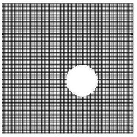
Figure 1: Sinai billiard graph

First we look at the nodal zone structure of one of the eigenfunctions – cf. Fig. 2. The vertices of the graph are marked as black when the value of the eigenfunction is positive at the vertex or white when it is negative. What comes out is a pattern similar to that of the hard-wall Schrödinger problem on the corresponding Sinai billiard.

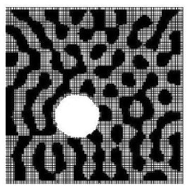
Figure 2: Nodal domains an eigenfunction

As we have indicated we want to compare transport properties of such systems in the situation when an incoming and outgoing lead is attached to the graph (at the points $(14,40)$ and $(59,80)$) and to the billiard at the corresponding places. Adding a lead to a graph, represents no problems: at the incoming / outgoing vertex a semiinfinite is added and the resulting five edges are again coupled by Kirchhoff conditions, (2.3) with $\alpha_{j}=0$. On the other hand, coupling a billiard to leads needs explanation. Here we use a standard method and describe the attached leads (attached antenna in the case of microwave billiards) by Sommerfeld radiation boundary conditions. Using this approach the attached lead is replaced by a small circle and the following boundary conditions are imposed on its boundary:

$${{\partial\psi}\over{\partial\overrightarrow{n}}}+ik\psi=2ik$$ (4.1)

for the incoming lead and

$${{\partial\psi}\over{\partial\overrightarrow{n}}}+ik\psi=0$$ (4.2)

for the outgoing one. The radius of the circles is much smaller then the length of graph bonds. We have used $r=0.01$ for the numerical tests. Another possibility is to relax the regularity requirement to solution $\phi$ to a two-dimensional Helmholtz equation at the junction points. This approach is formally equivalent to the limit $r\to 0$ and is described in ES2 , BG , etv and ES3 . However since we are interested in global structures that extend over the whole graph (billiard) the detail character of the connection is not important.

Let us start with comparing the wavefunctions on the graph with those obtained for the corresponding two-dimensional billiard. A typical result is displayed on the Figure 3 where we have plotted the absolute value of the wavefunction. For the graph, on the other hand, the values of the solution on the vertices are shown.

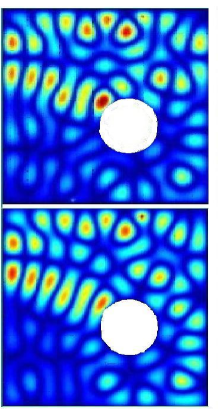
Figure 3: Eigenfunction comparison in terms of probability density. In the left picture squared modulus of the graph eigenfunction corresponds to energy $E$ referring to the momentum $k=1.65$. The right picture shows the same for billiard eigenfunction of energy $2E$. The color scale ranges from zero (dark blue) to the maximum value (dark red).

Speaking of phase-related effects, a primary quantity of interest is the probability current which in (an open) billiard is given conventionally by

$$\vec{\jmath}(\vec{x})=\mathrm{Im\,}\left(\bar{\psi}\nabla\psi\right)(\vec{x})$$ (4.3)

On the graph the current flows along the edges and has therefore a prescribed direction – cf. Fig. 4 – so it is not obvious what is the quantity to be compared to the two dimensional case. The natural possibility is to add the “horizontal” and “vertical” flows at each vertex by a vector summation and construct a in such a way a vector field. It turns out that leads indeed to the correct probability current inside the two dimensional billiard. We computed the currents using the above procedure are compared them with the current inside the two dimensional billiard that was evaluated with the help of the formula (4.3). The result is plotted on the Figure 5.

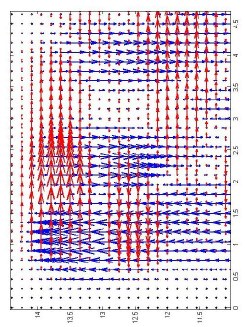
Figure 4: Probability currents on $\Gamma$

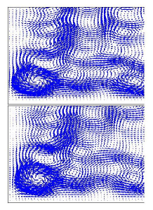
Figure 5: Determining the vector field. The left current is obtained by the vector summation while the current inside the billiard is plotted on the right side

In conclusion we have demonstrated the existence of global structures on large graphs. The structures do not depend on the local graph topology. We were able to prove that the large scale structures are the same on a square graph, where each vertex connects 4 bond, and on a graph consisting of equilateral triangles when 6 bonds are connected at each vertex. Moreover numerical results show that the structures do not change also for other types of graphs (although a rigorous proof is missing).

The structures extend over hundreds of graph vertices. They make up the manifestation of complex interference effects and are as such difficult to understand. The way out is to employ embedding of the graph into the appropriate ambient space and proving that the graph wavefunction converges to a corresponding solution of Schrödinger equation with the scaled energy.

- (1)
- (2) K. Ruedenberg, C.W. Scherr, J.Chem.Phys. 21, 1565 (1953).
- (3) J.E. Avron, A. Raveh, B. Zur, Rev.Mod.Phys. 60, 873 (1988)
- (4) P. Exner, P. Šeba, Rep. Math. Phys. 28, 7 (1989)
- (5) V. Kostrykin, R. Schrader, J. Phys. A: Math. Gen. 32, 595 (1999)
- (6) P. Kuchment, Waves in Random Media 12, R1 (2002)
- (7) S. Albeverio, F. Gesztesy, R. Høegh-Krohn, H. Holden, Solvable Models in Quantum Mechanics, 2nd edition, AMS Chelsea, Providence, R.I., 2005
- (8) G. Berkolaiko, E.B. Bogomolny, J.P. Keating, J. Phys. A: Math. Gen. 34, 335 (2001)
- (9) T. Kottos, U. Smilansky, Phys. Rev. Lett. 79, 4794 (1997)
- (10) T. Kottos, U. Smilansky, J. Phys. A: Math. Gen. 36, 3501 (2003)
- (11) O. Hul, S. Bauch, P. Pakonski, N. Savytskyy, K. Życzkowski, L. Sirko, Phys. Rev. E69, 056205 (2004)
- (12) G.G. Blasdel, J. Neuroscience 12, 3139 (1992)
- (13) F. Wolf, H.-U. Bauer, K. Pawelzik, T. Geisel, Nature 382, 306 (1996)
- (14) G. Blum, S. Gnutzmann, U. Smilansky, Phys. Rev. Lett. 88, 114101 (2002)
- (15) T. Biyikoglu, W. Hordijk, J. Leydold, T. Pisanski, P.F. Stadler, Lin. Alg. Appl. 390, 155 (2004)
- (16) T. Biyikoglu, Lin. Alg. Appl. 360, 197 (2003) - 205.
- (17) P. Exner, Ann. Inst. H. Poincaré: Phys. Théor. 66, 359 (1997)
- (18) Yu. Melnikov. B. Pavlov,J. Math. Phys. 42, 1202 (2001).
- (19) P. Exner, R. Gawlista, Phys. Rev. B53, 7275 (1996)
- (20) P. Exner, P. Šeba, J. Math. Phys. 28, 386 (1987)
- (21) J. Brüning, V.A. Geyler, J. Math. Phys. 44, 371 (2003)
- (22) P. Exner, M. Tater, D. Vaněk, J. Math. Phys. 42, 4050 (2001)
- (23) P. Exner, P. Šeba, Phys. Lett. A228, 146 (1997)