Repeat-Until-Success quantum computing using stationary and flying qubits

Abstract

We introduce an architecture for robust and scalable quantum computation using both stationary qubits (e.g. single photon sources made out of trapped atoms, molecules, ions, quantum dots, or defect centers in solids) and flying qubits (e.g. photons). Our scheme solves some of the most pressing problems in existing non-hybrid proposals, which include the difficulty of scaling conventional stationary qubit approaches, and the lack of practical means for storing single photons in linear optics setups. We combine elements of two previous proposals for distributed quantum computing, namely the efficient photon-loss tolerant build up of cluster states by Barrett and Kok [Phys. Rev. A 71, 060310 (2005)] with the idea of Repeat-Until-Success (RUS) quantum computing by Lim et al. [Phys. Rev. Lett. 95, 030505 (2005)]. This idea can be used to perform eventually deterministic two-qubit logic gates on spatially separated stationary qubits via photon pair measurements. Under non-ideal conditions, where photon loss is a possibility, the resulting gates can still be used to build graph states for one-way quantum computing. In this paper, we describe the RUS method, present possible experimental realizations, and analyse the generation of graph states.

I Introduction

Quantum computing offers a way to realize certain algorithms exponentially more efficiently than with the best known classical solutions shor ; deutsch . A substantial effort has therefore been made to develop the corresponding quantum technologies. Proof-of-principle experiments demonstrating the feasibility of quantum computing have already been performed: Using nuclear magnetic resonance techniques, Vandersypen et al. chuang realized a simple instance of Shor’s algorithm by factoring $15=3\times 5$. A two qubit gate has been implemented in a color center in diamond, utilizing the electron spin state of the nitrogen-vacancy defect center together with a nearby nuclear spin as qubits jelezko2004b . Groups in Innsbruck and Boulder implemented a universal two-qubit gate in an ion trap blatt ; wineland , and the three-qubit teleportation protocol blatt2 ; wineland2 . Adding more qubits to this “proto quantum computer” will increase the density of the motional states used for the two-qubit interaction. Consequently, it will become even harder to implement clean two-qubit gates. Scaling ion trap quantum computers much further therefore seems to require some form of distributed quantum information processing, possibly involving ion transport kielpinski .

The schemes mentioned above are based on manipulating stationary qubits such as atoms, molecules, or trapped ions. An alternative route to finding a feasible and scalable technology for building quantum computers is based on flying qubits, such as photons. The main advantage of photons is their extremely long coherence time: In vacuum and in simple dielectric media, photons do not interact with their environment, and hence do not lose their quantum information. This is why photons are usually the qubits of choice for quantum communication bennett ; ekert . However, at the same time this lack of interaction means that it is very hard to create two-photon entangling gates. It therefore came as a surprise that the bosonic symmetry requirement of the electromagnetic field, together with photon counting and proper single-photon sources, is sufficient for implementing scalable quantum computing KLM . The overhead cost for Linear Optical Quantum Computing (LOQC) has subsequently been brought down significantly. In particular, the one-way or cluster-state model for quantum computing raussendorf has allowed for drastic improvements in the scalability yoran03 ; nielsen04 ; browne04 . Recently, a four-qubit cluster state was realized experimentally by Walther et al. walther . The main drawbacks of LOQC are the difficulties of maintaining interferometric stability, the lack of practical ‘on demand’ single-photon sources and the lack of quantum memories for photonic qubits gingrich03 .

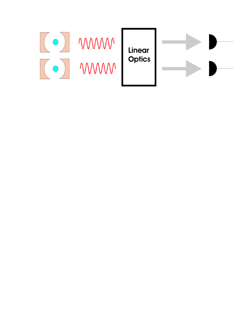
Figure 1: Experimental realization of a universal two-qubit gate for the considered network of single photon sources (stationary qubits). This requires the generation of a photon within each of the sources involved. The two photons then pass within their coherence time through a linear optics network, which performs a certain photon pair measurement.

In this paper, we consider the practical advantage of combining stationary and flying qubits for the realisation of scalable quantum computing. The stationary qubits (single photon sources) are arranged in a network of nodes with each node processing and storing a small number of qubits. To achieve scalability, the concept of distributed quantum computing was introduced and it was proposed that distant qubits communicate with each other through the means of flying qubits (i.e. photons) Grover ; Cirac . Initial schemes for the implementation of this idea relied on entangled ancillas as a resource Grover ; Cirac ; Jens ; duan04 ; taylor04 . Others required that the photon from one source is fed into another source cirac97 ; Enk ; Molmer ; meier04 ; Guo ; Zhou or a photon-mediated interaction between two fiber-coupled distant cavities needed to be established Bose . More hybrid approaches to quantum computing can be found in Refs. franson ; bill .

Other authors developed schemes for the probabilistic generation of highly entangled states between distant single photon sources cabrillo ; bose99 ; zoller ; last ; browne ; Simon ; lim ; Zou ; chim . In these schemes, one generates a photon in each of the sources and then performs an entangling photon measurement. By virtue of entanglement swapping, this results in entangled stationary qubits. It has been shown that similar ideas can also result in the implementation of probabilistic remote two-qubit gates grangier . At this point, it was believed that scalable quantum computing with distant photon sources requires additional resources such as local entangling gates duan04 or entangled ancillas in order to become deterministic.

The concrete setup that we consider in this paper has recently been introduced by Lim et al. moonlight and allows for the more efficient implementation of universal two-qubit gates than previous proposals. The presented scheme consists of a network of single stationary qubits (like trapped atoms, molecules, ions, quantum dots and nitrogen vacancy color centers) inside optical cavities, which act as a source for the generation of single photons on demand. Read-out measurements and single qubit rotations can be performed on the stationary qubits using laser pulses and standard quantum optics techniques as employed in the recent ion trap experiments in Innsbruck and Boulder blatt ; wineland .

The main building block for the realization of a two-qubit gate, which qualifies the setup for universal quantum computing, is shown in Figure 1. It requires the simultaneous generation of a photon in each source involved in the operation. Afterwards the photons should pass through a linear optics setup, where a pair measurement is performed in the output ports. This photon pair measurement results either in the completion of the gate or indicates the presence of the original qubits. In the later event, the gate should be repeated. The qubits are never lost in the computation and the presented scheme has therefore been called Repeat-Until-Success quantum computing moonlight .

Under realistic conditions, i.e. in the presence of finite detector efficiencies and finite success rates for the generation of a single photon on demand, the setup in Figure 1 can still be used for the implementation of probabilistic gates with a very high fidelity. As shown recently by Barrett and Kok Sean , it is possible to use probabilistic gates to efficiently generate graph states for one-way quantum computing raussendorf . Both schemes, moonlight and Sean overcome the limitations to scalable quantum computing faced before when using the same resources. In Ref. moonlight this is achieved with an eventually deterministic gate. Ref. Sean introduced a so-called double-heralding scheme, in which the entangling photo-detection stage was employed twice to eliminate unwanted separable contributions to the density matrix.

In this paper, we combine the ideas presented in our previous work moonlight ; Sean . In this way, we obtain a truly scalable design for quantum computing, i.e. even in the presence of imperfect components, with several key advantages:

1. Since our system uses no direct qubit-qubit interactions, the qubits can be well isolated. Not only does this allow us to address the individual qubits easily, it also means that there are fewer decoherence channels and hence fewer errors in the computation.

2. We achieve robustness to photon loss. In the presence of photon loss, the two qubit gates become non-deterministic. However, the gate failures are heralded, and so the gates can still be used to build high-fidelity entangled states, albeit in a non-deterministic manner. Photon loss thus increases the overall overhead cost associated with the scheme, but does not directly reduce the fidelity of the computation. When realistic photo-detectors and optical elements are used, photon loss is inevitable and this built-in robustness is essential.

3. Our scheme largely relies only on components that have been demonstrated in experiments like atom-photon entanglement Monroe ; weber . Apart from linear optics, we require only relatively good sources for the generation of single photons on demand Kuhn2 ; Yamamoto ; Mckeever ; Lange04 ; Kuzmich , preferrably at a high rate grangierscience , and relatively efficient but not necessarily number resolving photon detectors Rosenberg . Combining these in a working quantum computer will be challenging, but the basic physics has been shown to be correct.

4. The photon pair measurement is interferometrically stable. Since each generated photon contributes equally to the detection of a photon in the linear optics setup, fluctuations in the length between the photon source and the detectors can at most result in an overall phase factor with no physical consequences. This constitutes a significant advantage compared to previous schemes based on one-photon measurements (the only interferometrically stable schemes are last ; Simon ; lim ; moonlight ), since the photons do not need to arrive simultaneously in the detectors as long as they overlap within their coherence time in the setup.

5. The basic ideas presented in this paper are implementation independent and the stationary qubits can be realised in a variety of ways. Any system with the right energy-level structure and able to produce encoded flying qubits may be used.

6. Our scheme is inherently distributed. Hence, it can be used in applications which integrate both quantum computation and quantum communication. We show that entanglement can be generated directly between any two stationary qubits in the physical quantum computer. This significantly reduces the computational cost compared to architectures involving only nearest-neighbor interactions between the qubits gottesman2000 .

This paper is organized as follows. In the next Section, we give an overview on the basic principles of measurement-based quantum computing, since the described hybrid approach to quantum computing constitutes a novel implementation of these ideas. Section III details the general principle of a remote two-qubit gate implementation. In Section IV, we discuss possible gate implementations with polarization and time-bin encoded photons. In Section V, we describe how to overcome imperfections of inefficient photon generation and detection with the help of pre-fabricated graph states. Finally, we state our conclusions in Section VI.

II Measurement-based quantum computing

One condition for the successful implementation of a measurement-based quantum gate is that the measurement outcome is mutually unbiased Wootters with respect to the computational basis. In this way, an observer does not learn anything about the state of the qubits and the information might remain stored inside the computer. To avoid the destruction of qubits, it is not allowed to measure on the qubits directly. Measurements should only be performed on ancillas, which have interacted and therefore share entanglement with the qubits. These ancillas can be of the same physical realisation as the computational qubits nine ; fifteen ; raussendorf ; leung but they might also be realised differently. If the stationary qubits are atoms, the ancilla can be the quantised field mode inside an optical cavity beige , a common vibrational mode beige2 or newly generated photons, as in the setup considered here. Vice versa, it has been found advantageous to use collective atomic states as ancillas for photonic qubits franson ; bill .

Let us now briefly describe the principles of measurement-based quantum computing in a more formal way. Using the terms ‘qubits’ and ‘ancillas’ provides a convenient picture, which is especially suited for the description of hybrid approaches, where the qubits may remain encoded in the same physical qubits instead of being assigned dynamically as the computation proceeds. As in Ref. kok , we consider two systems, $s$ and $a$, that are initially in the state ($c_{n}\in\mathbb{C}$)

$$|\Psi\rangle_{s}|A_{0}\rangle_{a}\equiv\sum_{n}c_{n}|\psi_{n}\rangle_{s}\otimes|A_{0}\rangle_{a}\,.$$ (1)

After some interaction, the joint system evolves into

$$|\Psi\rangle_{s}|A_{0}\rangle_{a}\rightarrow\sum_{n}c_{n}|\psi_{n}\rangle_{s}\otimes|A_{n}\rangle_{a}\equiv|\Phi\rangle\,,$$ (2)

where the $|A_{n}\rangle_{a}$ are the eigenstates of an observable $\mathsf{A}$. We can then measure $\mathsf{A}$, which will reveal the state of the system $s$. This can be interpreted as a quantum non-demolition measurement of $s$ but this is not what we are interested in here.

In this article we will instead consider measurements of an observable $\mathsf{B}$, as shown in Figure 2, that is complementary to $\mathsf{A}$. In other words, the eigenvectors of $\mathsf{A}$ and $\mathsf{B}$ form a so-called mutually unbiased basis of the Hilbert space of system $a$. A specific outcome labelled $k$ of such a measurement corresponds to the application of the projection operator $\hat{B}_{k}$ (associated with the $k^{\mathrm{th}}$ eigenvector of $\mathsf{B}$), and the state of system $s$ is then given by

$$|\Upsilon_{k}\rangle_{s}=\frac{\text{Tr}_{a}\left[\langle\Phi|\mbox{\small 1}\!\!\mbox{1}\otimes\hat{B}_{k}|\Phi\rangle\right]}{\text{Tr}_{sa}\left[\langle\Phi|\mbox{\small 1}\!\!\mbox{1}\otimes\hat{B}_{k}|\Phi\rangle\right]}\,.$$ (3)

This can be generalized to situations where $\hat{B}_{k}$ is a multi-rank projector or a Positive Operator Valued Measure (POVM). The conditions for the evolution $|\psi_{n}\rangle_{s}\to|\Upsilon_{k}\rangle_{s}$ to be a unitary transformation on system $s$ are presented in Lapaire et al. kok . If $s$ describes the qubits and $a$ the ancilla, they guarantee, as mentioned above, that the detection of $\hat{B}_{k}$ does not reveal any information about the qubits.

Especially, in the setup considered in this paper the system $s$ consists of a set of $N$ stationary qubits occupying a Hilbert space of size $2^{N}$, and system $a$ consists of $N$ flying quantum systems occupying a Hilbert space of dimension $d\geq 2^{N}$. A measurement of the observable $\mathsf{B}$ on the flying qubits will result in a multi-qubit (entangling) operation on the stationary qubits. We are interested in the case where the projector $\hat{B}_{k}$ induces a unitary transformation on the stationary qubits,

$$|\Upsilon_{k}\rangle_{s}=U_{k}|\Psi\rangle_{s}\,,$$ (4)

which means that $\hat{B}_{k}$ is a proper projector. There are two interesting cases to consider:

1. The set $\{\hat{B}_{k}\}_{a}$ corresponds to a basis of states that induces a complete set $\{U_{k}\}_{a}$ of entangling quantum gates. As a result, finding any measurement outcome $k$ will induce a unitary entangling gate operation on the stationary qubits.

2. The set $\{\hat{B}_{k}\}_{a}$ corresponds to a basis that can be divided into two sets of states: Some of the projectors will induce a unitary entangling gate $U_{k}$ on the stationary qubits, while the remaining projectors induce a transformation that is locally equivalent to the identity map 11.

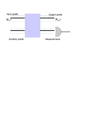
Figure 2: Measurement-based quantum computing. The input state $|\Psi\rangle_{s}$ and the auxiliary state $|A_{0}\rangle_{a}$ are transformed in an $N$-port that induces a unitary transformation $U_{sf}$. Given a detector outcome corresponding to a POVM $\hat{B}_{k}$, the output state is $|\Upsilon_{k}\rangle_{s}$.

The second setup is interesting for the following reason: Suppose that system $s$ consists of $N$ non-interacting (e.g., well-separated) stationary qubits with long decoherence times. If this system can generate flying qubits in the manner described above, we can perform a measurement of the observable $\mathsf{B}$ and entangle the non-interacting stationary qubits. When not all measurement outcomes produce an entangling gate on the stationary qubits (some yield instead the identity operator), then the unitary gate is applied only part of the time. However, due to the fact that a gate failure corresponds to an identity operation (or something locally equivalent), we can again prepare the flying qubits in the state $|A_{0}\rangle_{a}$. This allows us to repeat the protocol until the entangling gate is applied successfully, which is why we called this idea Repeat-Until-Success quantum computing moonlight .

III Remote two-qubit phase gates

One of the requirements for universal quantum computing is the ability to perform an entangling two-qubit gate operation, like a controlled phase gate divincenzo . In this Section we describe the general concept for the implementation of this gate between two distant single photon sources. Note that our method of distributed quantum computing allows to realize entangling operations, since the measurement on a photon pair can imprint a phase on the state of its sources although it cannot change the distribution of their populations. The first step for the implementation of a two-qubit gate is the generation of a photon within each respective source, which encodes the information of the stationary qubit.

III.1 Encoding

Let us denote the states of the photon sources, which encode the logical qubits $|0\rangle_{\rm L}$ and $|1\rangle_{\rm L}$ as $|0\rangle$ and $|1\rangle$, respectively. An arbitrary pure state of two stationary qubits can then be written as

$$|\psi_{\rm in}\rangle=\alpha\,|00\rangle+\beta\,|01\rangle+\gamma\,|10\rangle+\delta\,|11\rangle\,,$$ (5)

where $\alpha$, $\beta$, $\gamma$ and $\delta$ are complex coefficients with $|\alpha|^{2}+|\beta|^{2}+|\gamma|^{2}+|\delta|^{2}=1$. Suppose that a photon is generated in each of the two sources, whose state (i.e. its polarization or generation time) depends on the state of the respective source. In the following we assume that source 1 prepared in $|i\rangle$ leads to the creation of one photon in state $|{\sf x}_{i}\rangle$, while source 2 prepared in $|i\rangle$ leads to the creation of one photon in state $|{\sf y}_{i}\rangle$,

$$|i\rangle_{1}\rightarrow|i,{\sf x}_{i}\rangle_{1}\,,~{}~{}|i\rangle_{2}\rightarrow|i,{\sf y}_{i}\rangle_{2}\,.$$ (6)

The simultaneous creation of a photon in both sources then transfers the initial state (5) into

$$|\psi_{\rm enc}\rangle = \alpha\,|00,{\sf x}_{0}{\sf y}_{0}\rangle+\beta\,|01,{\sf x}_{0}{\sf y}_{1}\rangle+\gamma\,|10,{\sf x}_{1}{\sf y}_{0}\rangle$$ (7)

$$+\delta\,|11,{\sf x}_{1}{\sf y}_{1}\rangle\,.$$

Note that the generation of photons whose state depends on the states of the stationary qubits is a highly non-linear process. The preparation of the generally entangled state (7) is indeed the key step which allows the completion of an eventually deterministic two-qubit gate with otherwise nothing else than linear optics and photon pair measurements. The way the encoding step (6) can be realized experimentally is discussed in Section IV. In this section we focus on the general ideas underlying Repeat-Until-Success quantum computing.

III.2 Mutually Unbiased Basis

Once the photons have been created, an entangling phase gate can be implemented by performing an absorbing measurement on the photon pair. Thereby, it is important to choose the photon measurement such that none of the possible outcomes reveals any information about the coefficients $\alpha$, $\beta$, $\gamma$ and $\delta$, as mentioned in Section II. This can be achieved with a photon pair measurements in a basis mutually unbiased Wootters with respect to the computational basis given by the states $\{|{\sf x}_{0}{\sf y}_{0}\rangle,\,|{\sf x}_{0}{\sf y}_{1}\rangle,\,|{\sf x}_{1}{\sf y}_{0}\rangle,\,|{\sf x}_{1}{\sf y}_{1}\rangle\}$. More concretely, all possible outcomes of the photon measurement should be of the form

$$|\Phi\rangle={\textstyle{1\over 2}}\big{[}|{\sf x}_{0}{\sf y}_{0}\rangle+{\rm e}^{{\rm i}\varphi_{1}}\,|{\sf x}_{0}{\sf y}_{1}\rangle+{\rm e}^{{\rm i}\varphi_{2}}\,|{\sf x}_{1}{\sf y}_{0}\rangle+{\rm e}^{{\rm i}\varphi_{3}}\,|{\sf x}_{1}{\sf y}_{1}\rangle\big{]}\,.$$ (8)

As we see below, a complete set of basis states of this form can be found. Any bias in the amplitudes would yield information about $\alpha$, $\beta$, $\gamma$, and $\delta$, and would therefore not induce a unitary gate on the stationary qubits. Detecting the state (8) and absorbing the two photons in the process transfers the encoded state (7) into

$$|\psi_{\rm out}\rangle = \alpha\,|00\rangle+{\rm e}^{-{\rm i}\varphi_{1}}\,\beta\,|01\rangle+{\rm e}^{-{\rm i}\varphi_{2}}\,\gamma\,|10\rangle$$ (9)

$$+{\rm e}^{-{\rm i}\varphi_{3}}\,\delta\,|11\rangle\,.$$

Note that the output state (9) differs from the initial state (5) by a two-qubit phase gate.

Let us now consider the angle

$$\varphi_{3}=\varphi_{1}+\varphi_{2}\,.$$ (10)

In this case, the state $|\Phi\rangle$ is a product state and the output (9) differs from the initial state (5) only by local operations. However, if

$$\varphi_{3}=\varphi_{1}+\varphi_{2}+\pi\,,$$ (11)

the state (8) becomes a maximally entangled state, as it becomes obvious when writing $|\Phi\rangle$ as

$$|\Phi\rangle={\textstyle{1\over 2}}\big{[}|{\sf x}_{0}\rangle(|{\sf y}_{0}\rangle+{\rm e}^{{\rm i}\varphi_{1}}\,|{\sf y}_{1}\rangle)+{\rm e}^{{\rm i}\varphi_{2}}\,|{\sf x}_{1}\rangle(|{\sf y}_{0}\rangle-{\rm e}^{{\rm i}\varphi_{1}}\,|{\sf y}_{1}\rangle)\big{]}\,.$$ (12)

The detection of a photon pair in this maximally entangled state results in the completion of a phase gate with maximum entangling power on the stationary qubit. Vice versa, maximum entanglement of the state (8) also automatically implies Eq. (11) as one can show by calculating the entanglement of formation of the state (8).

III.3 A deterministic gate

In the following, we denote the states of the measurement basis, i.e. the mutually unbiased basis, by $\{|\Phi_{i}\rangle\}$. In order to find a complete Bell basis with all states of form (8), we define

$$|\Phi_{1}\rangle \equiv {\textstyle{1\over\sqrt{2}}}\big{[}|{\sf a}_{1}{\sf b}_{1}\rangle+|{\sf a}_{2}{\sf b}_{2}\rangle\big{]}\,,$$

$$|\Phi_{2}\rangle \equiv {\textstyle{1\over\sqrt{2}}}\big{[}|{\sf a}_{1}{\sf b}_{1}\rangle-|{\sf a}_{2}{\sf b}_{2}\rangle\big{]}\,,$$

$$|\Phi_{3}\rangle \equiv {\textstyle{1\over\sqrt{2}}}\big{[}|{\sf a}_{1}{\sf b}_{2}\rangle+|{\sf a}_{2}{\sf b}_{1}\rangle\big{]}\,,$$

$$|\Phi_{4}\rangle \equiv {\textstyle{1\over\sqrt{2}}}\big{[}|{\sf a}_{1}{\sf b}_{2}\rangle-|{\sf a}_{2}{\sf b}_{1}\rangle\big{]}\,,$$ (13)

where the states $|{\sf a}_{i}\rangle$ describe photon 1 and the $|{\sf b}_{i}\rangle$ describe photon 2. Assuming orthogonality, i.e. $\langle{\sf a}_{1}|{\sf a}_{2}\rangle=0$ and $\langle{\sf b}_{1}|{\sf b}_{2}\rangle=0$, one can write the photon states on the right hand side of Eq. (III.3) without loss of generality as

$$|{\sf a}_{1}\rangle = c_{1}\,|{\sf x}_{0}\rangle+{\rm e}^{{\rm i}\vartheta_{1}}s_{1}\,|{\sf x}_{1}\rangle\,,$$

$$|{\sf a}_{2}\rangle = {\rm e}^{-{\rm i}\xi_{1}}({\rm e}^{-{\rm i}\vartheta_{1}}s_{1}\,|{\sf x}_{0}\rangle-c_{1}\,|{\sf x}_{1}\rangle)\,,$$

$$|{\sf b}_{1}\rangle = c_{2}\,|{\sf y}_{0}\rangle+{\rm e}^{{\rm i}\vartheta_{2}}s_{2}\,|{\sf y}_{1}\rangle\,,$$

$$|{\sf b}_{2}\rangle = {\rm e}^{-{\rm i}\xi_{2}}({\rm e}^{-{\rm i}\vartheta_{2}}s_{2}\,|{\sf y}_{0}\rangle-c_{2}\,|{\sf y}_{1}\rangle)$$ (14)

with

$$s_{i}\equiv\sin{\theta_{i}}\,,~{}~{}c_{i}\equiv\cos{\theta_{i}}\,.$$ (15)

Inserting this into Eq. (III.3), we find

$$|\Phi_{1}\rangle = {\textstyle{1\over\sqrt{2}}}\big{[}\big{(}c_{1}c_{2}+{\rm e}^{-{\rm i}(\vartheta_{1}+\vartheta_{2})}{\rm e}^{-{\rm i}(\xi_{1}+\xi_{2})}s_{1}s_{2}\big{)}|{\sf x}_{0}{\sf y}_{0}\rangle+\big{(}{\rm e}^{{\rm i}\vartheta_{2}}c_{1}s_{2}-{\rm e}^{-{\rm i}\vartheta_{1}}{\rm e}^{-{\rm i}(\xi_{1}+\xi_{2})}s_{1}c_{2}\big{)}|{\sf x}_{0}{\sf y}_{1}\rangle$$

$$+\big{(}{\rm e}^{{\rm i}\vartheta_{1}}s_{1}c_{2}-{\rm e}^{-{\rm i}\vartheta_{2}}{\rm e}^{-{\rm i}(\xi_{1}+\xi_{2})}c_{1}s_{2}\big{)}|{\sf x}_{1}{\sf y}_{0}\rangle+\big{(}{\rm e}^{{\rm i}(\vartheta_{1}+\vartheta_{2})}s_{1}s_{2}+{\rm e}^{-{\rm i}(\xi_{1}+\xi_{2})}c_{1}c_{2}\big{)}|{\sf x}_{1}{\sf y}_{1}\rangle\big{]},$$

$$|\Phi_{2}\rangle = {\textstyle{1\over\sqrt{2}}}\big{[}\big{(}c_{1}c_{2}-{\rm e}^{-{\rm i}(\vartheta_{1}+\vartheta_{2})}{\rm e}^{-{\rm i}(\xi_{1}+\xi_{2})}s_{1}s_{2}\big{)}|{\sf x}_{0}{\sf y}_{0}\rangle+\big{(}{\rm e}^{{\rm i}\vartheta_{2}}c_{1}s_{2}+{\rm e}^{-{\rm i}\vartheta_{1}}{\rm e}^{-{\rm i}(\xi_{1}+\xi_{2})}s_{1}c_{2}\big{)}|{\sf x}_{0}{\sf y}_{1}\rangle$$

$$+\big{(}{\rm e}^{{\rm i}\vartheta_{1}}s_{1}c_{2}+{\rm e}^{-{\rm i}\vartheta_{2}}{\rm e}^{-{\rm i}(\xi_{1}+\xi_{2})}c_{1}s_{2}\big{)}|{\sf x}_{1}{\sf y}_{0}\rangle+\big{(}{\rm e}^{{\rm i}(\vartheta_{1}+\vartheta_{2})}s_{1}s_{2}-{\rm e}^{-{\rm i}(\xi_{1}+\xi_{2})}c_{1}c_{2}\big{)}|{\sf x}_{1}{\sf y}_{1}\rangle\big{]},$$

$$|\Phi_{3}\rangle = {\textstyle{1\over\sqrt{2}}}\big{[}\big{(}{\rm e}^{-{\rm i}\vartheta_{2}}{\rm e}^{-{\rm i}\xi_{2}}c_{1}s_{2}+{\rm e}^{-{\rm i}\vartheta_{1}}{\rm e}^{-{\rm i}\xi_{1}}s_{1}c_{2}\big{)}|{\sf x}_{0}{\sf y}_{0}\rangle-\big{(}{\rm e}^{-{\rm i}\xi_{2}}c_{1}c_{2}-{\rm e}^{-{\rm i}(\vartheta_{1}-\vartheta_{2})}{\rm e}^{-{\rm i}\xi_{1}}s_{1}s_{2}\big{)}|{\sf x}_{0}{\sf y}_{1}\rangle$$

$$+\big{(}{\rm e}^{{\rm i}(\vartheta_{1}-\vartheta_{2})}{\rm e}^{-{\rm i}\xi_{2}}s_{1}s_{2}-{\rm e}^{-{\rm i}\xi_{1}}c_{1}c_{2}\big{)}|{\sf x}_{1}{\sf y}_{0}\rangle-\big{(}{\rm e}^{{\rm i}\vartheta_{1}}{\rm e}^{-{\rm i}\xi_{2}}s_{1}c_{2}+{\rm e}^{{\rm i}\vartheta_{2}}{\rm e}^{-{\rm i}\xi_{1}}c_{1}s_{2}\big{)}|{\sf x}_{1}{\sf y}_{1}\rangle\big{]},$$

$$|\Phi_{4}\rangle = {\textstyle{1\over\sqrt{2}}}\big{[}\big{(}{\rm e}^{-{\rm i}\vartheta_{2}}{\rm e}^{-{\rm i}\xi_{2}}c_{1}s_{2}-{\rm e}^{-{\rm i}\vartheta_{1}}{\rm e}^{-{\rm i}\xi_{1}}s_{1}c_{2}\big{)}|{\sf x}_{0}{\sf y}_{0}\rangle-\big{(}{\rm e}^{-{\rm i}\xi_{2}}c_{1}c_{2}+{\rm e}^{-{\rm i}(\vartheta_{1}-\vartheta_{2})}{\rm e}^{-{\rm i}\xi_{1}}s_{1}s_{2}\big{)}|{\sf x}_{0}{\sf y}_{1}\rangle$$

$$+\big{(}{\rm e}^{{\rm i}(\vartheta_{1}-\vartheta_{2})}{\rm e}^{-{\rm i}\xi_{2}}s_{1}s_{2}+{\rm e}^{-{\rm i}\xi_{1}}c_{1}c_{2}\big{)}|{\sf x}_{1}{\sf y}_{0}\rangle-\big{(}{\rm e}^{{\rm i}\vartheta_{1}}{\rm e}^{-{\rm i}\xi_{2}}s_{1}c_{2}-{\rm e}^{{\rm i}\vartheta_{2}}{\rm e}^{-{\rm i}\xi_{1}}c_{1}s_{2}\big{)}|{\sf x}_{1}{\sf y}_{1}\rangle\big{]}.$$

These states are of the form (8), if the amplitudes are all of the same size, which yields the conditions

$$\big{|}c_{1}c_{2}\pm{\rm e}^{-{\rm i}(\vartheta_{1}+\vartheta_{2}+\xi_{1}+\xi_{2})}s_{1}s_{2}\big{|}$$ (17)

$$= \big{|}c_{1}s_{2}\pm{\rm e}^{-{\rm i}(\vartheta_{1}+\vartheta_{2}+\xi_{1}+\xi_{2})}s_{1}c_{2}\big{|}=\textstyle{1\over\sqrt{2}}\,,$$

and

$$\big{|}c_{1}s_{2}\pm{\rm e}^{-{\rm i}(\vartheta_{1}-\vartheta_{2}+\xi_{1}-\xi_{2})}s_{1}c_{2}\big{|}$$ (18)

$$= \big{|}c_{1}c_{2}\pm{\rm e}^{-{\rm i}(\vartheta_{1}-\vartheta_{2}+\xi_{1}-\xi_{2})}s_{1}s_{2}|=\textstyle{1\over\sqrt{2}}\,.$$

The only solution of the constraints (17) and (18) is

$$\cos(2\theta_{1})\cos(2\theta_{2})=\cos(\vartheta_{1}\pm\vartheta_{2}+\xi_{1}\pm\xi_{2})=0$$ (19)

provided that neither $\cos(2\theta_{1})$ nor $\cos(2\theta_{2})$ equals 1. In the special case, where either $\cos(2\theta_{1})=1$ or $\cos(2\theta_{2})=1$, condition (19) simplifies to $\cos(2\theta_{1})\cos(2\theta_{2})=0$ with no restrictions in the angles $\vartheta_{1}$, $\vartheta_{2}$, $\xi_{1}$ and $\xi_{2}$.

One particular way to fulfill the restrictions (19) is to set

$$\xi_{2}=-{\textstyle{1\over 2}}\pi\,,~{}\xi_{1}=\vartheta_{1}=\vartheta_{2}=0~{}~{}{\rm and}~{}~{}\theta_{1}=\theta_{2}={\textstyle{1\over 4}}\pi\,,$$ (20)

which corresponds to the choice (c.f. moonlight )

$$|{\sf a}_{1}\rangle = {\textstyle{1\over\sqrt{2}}}(|{\sf x}_{0}\rangle+\,|{\sf x}_{1}\rangle)\,,$$

$$|{\sf a}_{2}\rangle = {\textstyle{1\over\sqrt{2}}}(|{\sf x}_{0}\rangle-\,|{\sf x}_{1}\rangle)\,,$$

$$|{\sf b}_{1}\rangle = {\textstyle{1\over\sqrt{2}}}(|{\sf y}_{0}\rangle+|{\sf y}_{1}\rangle)\,,$$

$$|{\sf b}_{2}\rangle = {\textstyle{{\rm i}\over\sqrt{2}}}(|{\sf y}_{0}\rangle-|{\sf y}_{1}\rangle)$$ (21)

and yields

$$|\Phi_{1}\rangle = {\textstyle{1\over 2}}{\rm e}^{{\rm i}\pi/4}\big{[}|\sf x_{0}y_{0}\rangle-{\rm i}|\sf x_{0}y_{1}\rangle-{\rm i}|\sf x_{1}y_{0}\rangle+|\sf x_{1}y_{1}\rangle\big{]}\,,$$

$$|\Phi_{2}\rangle = {\textstyle{1\over 2}}{\rm e}^{-{\rm i}\pi/4}\big{[}|\sf x_{0}y_{0}\rangle+{\rm i}|\sf x_{0}y_{1}\rangle+{\rm i}|\sf x_{1}y_{0}\rangle+|\sf x_{1}y_{1}\rangle\big{]}\,,$$

$$|\Phi_{3}\rangle = {\textstyle{1\over 2}}{\rm e}^{{\rm i}\pi/4}\big{[}|\sf x_{0}y_{0}\rangle-{\rm i}|\sf x_{0}y_{1}\rangle+{\rm i}|\sf x_{1}y_{0}\rangle-|\sf x_{1}y_{1}\rangle\big{]}\,,$$

$$|\Phi_{4}\rangle = -{\textstyle{1\over 2}}{\rm e}^{-{\rm i}\pi/4}\big{[}|\sf x_{0}y_{0}\rangle+{\rm i}|\sf x_{0}y_{1}\rangle-{\rm i}|\sf x_{1}y_{0}\rangle-|\sf x_{1}y_{1}\rangle\big{]}\,.$$

To find out which gate operation the detection of the corresponding maximally entangled states (III.3) combined with a subsequent absorption of the photon pair results into, we write the input state (7) as

$$|\psi_{\rm enc}\rangle={\textstyle{1\over 2}}\sum_{i}^{4}|\psi_{i}\rangle\otimes|\Phi_{i}\rangle$$ (23)

and determine the states $|\psi_{i}\rangle$ of the stationary qubits. Using the notation

$$U_{\rm CZ} \equiv |00\rangle\langle 00|+|01\rangle\langle 01|+|10\rangle\langle 10|-|11\rangle\langle 11|~{}~{}~{}$$ (24)

for the controlled two-qubit phase gate (the CZ gate) and the notation

$$Z_{i}(\phi)\equiv|0\rangle_{\rm ii}\langle 0|+{\rm e}^{-{\rm i}\phi}|1\rangle_{\rm ii}\langle 1|$$ (25)

for the local controlled-Z gate on photon source $i$ endnote , we find

$$|\psi_{1}\rangle = \exp\big{(}{-\textstyle{1\over 4}}{\rm i}\pi\big{)}\,Z_{2}\big{(}-{\textstyle{1\over 2}}\pi\big{)}\,Z_{1}\big{(}-{\textstyle{1\over 2}}\pi\big{)}\,U_{\rm CZ}\,|\psi_{\rm in}\rangle\,,$$

$$|\psi_{2}\rangle = \exp\big{(}{\textstyle{1\over 4}}{\rm i}\pi\big{)}\,Z_{2}\big{(}{\textstyle{1\over 2}}\pi\big{)}\,Z_{1}\big{(}{\textstyle{1\over 2}}\pi\big{)}\,U_{\rm CZ}\,|\psi_{\rm in}\rangle\,,$$

$$|\psi_{3}\rangle = \exp\big{(}{-\textstyle{1\over 4}}{\rm i}\pi\big{)}\,Z_{2}\big{(}-{\textstyle{1\over 2}}\pi\big{)}\,Z_{1}\big{(}{\textstyle{1\over 2}}\pi\big{)}\,U_{\rm CZ}\,|\psi_{\rm in}\rangle\,,$$

$$|\psi_{4}\rangle = -\exp\big{(}{\textstyle{1\over 4}}{\rm i}\pi\big{)}\,Z_{2}\big{(}{\textstyle{1\over 2}}\pi\big{)}\,Z_{1}\big{(}-{\textstyle{1\over 2}}\pi\big{)}\,U_{\rm CZ}\,|\psi_{\rm in}\rangle\,.$$

From this we see that one can indeed obtain the CZ gate operation (24) up to local unitary operations upon the detection of any of the four Bell states $|\Phi_{i}\rangle$, as it has been pointed out already by Protsenko et al. grangier .

III.4 Repeat-Until-Success quantum computing

When implementing distributed quantum computing with photons as flying qubits, the problem arises that it is impossible to perform a complete deterministic Bell measurement on the photons using only linear optics elements. As it has been shown Lutkenhaus , in the best case, one can distinguish two of the four Bell states. Since the construction of efficient non-linear optical elements remains experimentally challenging, the above described phase gate could therefore be operated at most with success rate ${1\over 2}$.

What must be done to solve this problem is to choose the photon pair measurement basis $\{|\Phi_{i}\rangle\}$ such that two of the basis states are maximally entangled while the other two basis states are product states. Most importantly, all basis states must be mutually unbiased with respect to the computational basis and information will not be destroyed at any stage of the computation. In the following we choose $|\Phi_{3}\rangle$ and $|\Phi_{4}\rangle$ as in Eq. (III.3) and $|\Phi_{1}\rangle$ and $|\Phi_{2}\rangle$ as product states such that

$$|\Phi_{1}\rangle = |{\sf a_{1}b_{1}}\rangle\,,~{}~{}|\Phi_{2}\rangle=|{\sf a_{2}b_{2}}\rangle\,,$$

$$|\Phi_{3}\rangle \equiv {\textstyle{1\over\sqrt{2}}}\big{[}|{\sf a}_{1}{\sf b}_{2}\rangle+|{\sf a}_{2}{\sf b}_{1}\rangle\big{]}\,,$$

$$|\Phi_{4}\rangle \equiv {\textstyle{1\over\sqrt{2}}}\big{[}|{\sf a}_{1}{\sf b}_{2}\rangle-|{\sf a}_{2}{\sf b}_{1}\rangle\big{]}\,.$$ (27)

The aim of this is (see Section II) that in the event of the “failure” of the gate implementation (i.e. in case of the detection of $|\Phi_{1}\rangle$ or $|\Phi_{2}\rangle$) the system remains, up to a local phase gate, in the original qubit state. This means that the initial state (5) can be restored and the described protocol can be repeated, thereby eventually resulting in the performance of the universal controlled phase gate (24). The probability for the realization of the gate operation within one step equals ${1\over 2}$ and the final completion of a quantum phase gate therefore requires on average two repetitions of the above described photon pair generation and detection process.

Let us now determine the conditions under which the states $\{|\Phi_{i}\rangle\}$ are of the form (8). Proceeding as above, we find that the angles $\vartheta_{i}$, $\xi_{i}$ and $\theta_{i}$ in Eq. (III.3) should fulfill, for example, Eq. (20). In analogy to Eqs. (17) and (18), we find that $|\Phi_{1}\rangle$ and $|\Phi_{2}\rangle$ are mutually unbiased, if

$$\big{|}c_{1}c_{2}\big{|}=\big{|}c_{1}s_{2}\big{|}=\big{|}s_{1}c_{2}\big{|}=\big{|}s_{1}s_{2}\big{|}=\textstyle{1\over 2}\,,$$ (28)

which also holds for the parameter choice in Eq. (20). Using Eq. (III.3), one can easily verify that with the above choice the basis (III.4) becomes

$$|\Phi_{1}\rangle = {\textstyle{1\over 2}}\big{[}|\sf x_{0}y_{0}\rangle+|\sf x_{0}y_{1}\rangle+|\sf x_{1}y_{0}\rangle+|\sf x_{1}y_{1}\rangle\big{]}\,,$$

$$|\Phi_{2}\rangle = {\textstyle{{\rm i}\over 2}}\big{[}|\sf x_{0}y_{0}\rangle-|\sf x_{0}y_{1}\rangle-|\sf x_{1}y_{0}\rangle+|\sf x_{1}y_{1}\rangle\big{]}\,,$$

$$|\Phi_{3}\rangle = {\textstyle{1\over 2}}{\rm e}^{{\rm i}\pi/4}\big{[}|\sf x_{0}y_{0}\rangle-{\rm i}|\sf x_{0}y_{1}\rangle+{\rm i}|\sf x_{1}y_{0}\rangle-|\sf x_{1}y_{1}\rangle\big{]}\,,$$

$$|\Phi_{4}\rangle = -{\textstyle{1\over 2}}{\rm e}^{-{\rm i}\pi/4}\big{[}|\sf x_{0}y_{0}\rangle+{\rm i}|\sf x_{0}y_{1}\rangle-{\rm i}|\sf x_{1}y_{0}\rangle-|\sf x_{1}y_{1}\rangle\big{]}\,.$$

Choosing the states $|{\sf a}_{i}\rangle$ and $|{\sf b}_{i}\rangle$ as in Eq. (III.3) allows to implement the gate operation (24) eventually deterministically.

Finally, we determine the gate operations corresponding to the detection of a certain measurement outcome $|\Phi_{i}\rangle$. To do this, we decompose the input state (7) again into a state of the form (23). Proceeding as in the previous subsection, we find

$$|\psi_{1}\rangle = |\psi_{\rm in}\rangle\,,$$

$$|\psi_{2}\rangle = -{\rm i}\,Z_{2}\big{(}\pi\big{)}\,Z_{2}\big{(}\pi\big{)}\,|\psi_{\rm in}\rangle\,,$$

$$|\psi_{3}\rangle = \exp\big{(}{-\textstyle{1\over 4}}{\rm i}\pi\big{)}\,Z_{2}\big{(}-{\textstyle{1\over 2}}\pi\big{)}\,Z_{1}\big{(}{\textstyle{1\over 2}}\pi\big{)}\,U_{\rm CZ}\,|\psi_{\rm in}\rangle\,,$$

$$|\psi_{4}\rangle = -\exp\big{(}{\textstyle{1\over 4}}{\rm i}\pi\big{)}\,Z_{2}\big{(}{\textstyle{1\over 2}}\pi\big{)}\,Z_{1}\big{(}-{\textstyle{1\over 2}}\pi\big{)}\,U_{\rm CZ}\,|\psi_{\rm in}\rangle\,.$$

Again one obtains the CZ gate operation (24) up to local unitary operations upon the detection of either $|\Phi_{3}\rangle$ or $|\Phi_{4}\rangle$. In the event of the detection of the product states $|\Phi_{1}\rangle$ or $|\Phi_{2}\rangle$, the initial state can be restored with the help of one-qubit phase gates, which then allows us to repeat the operation until success.

It should be emphasized that there are other possible encodings that yield a universal two-qubit phase gate upon the detection of a Bell-state, but where the original state is destroyed upon the detection of a product state (see e.g. Zou ). This happens when the product states are not mutually unbiased and their detection erases the qubit states in the respective photon sources. To achieve the effect of an insurance against failure, the encoding (6) should be chosen as described in this Section.

IV Possible experimental realizations

Possible experimental realizations of the above described eventually deterministic quantum phase gate consist of two basic steps. Firstly, the information of the stationary qubits involved in the operation has to be redundantly encoded in the states of two newly generated ancilla photons. Afterwards, a measurement is performed on the photon pair resulting with probability ${1\over 2}$ in the desired gate operation. Depending on the type of the photon source, one can choose different types of encoding. There are also different possibilities how to perform the photon pair measurement. Examples are given below.

IV.1 Redundant encoding

In order to obtain robust qubits, the states $|0\rangle$ and $|1\rangle$ should be two different longliving ground states of the single photon source. Each photon source carries one qubit. Depending on its level structure (see Figure 3), it might be advantageous to realise the encoding step (7) either by generating photons with different polarisations (polarisation encoding) or photons that agree in all degrees of freedom apart from their creation time (time bin encoding). Note that different encodings can easily be transformed into each other using linear optics elements like a polarising beam splitters and delaying photons in time.

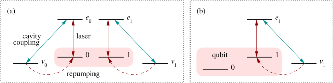
Figure 3: Schematic view of a single photon (a) polarization encoder, Ê(b) time-bin encoder and level configuration of the sourceÊ Êcontaining the qubit.

Polarization encoding. Suppose, the photon source contains an atomic double $\Lambda$ level configuration as shown in Figure 3(a) (see also Ref. Gheri ). A single photon can then be created by simultaneously applying a laser pulse with increasing Rabi frequency to the $0$-$e_{0}$ transition and the $1$-$e_{1}$ transition of the atomic system. Thereby, the atom goes to the ground state $|v_{0}\rangle$ and $|v_{1}\rangle$, respectively, depending on whether its initial state equalled $|0\rangle$ or $|1\rangle$ due to the coupling of the $e_{0}$-$v_{0}$ transition and the $e_{1}$-$v_{1}$ transition to the cavity mode. It has been shown in the past that this technique Law is very well suited to place exactly one excitation into the field of an optical resonator, from where it can leak out Kuhn2 .

If the two transitions, $e_{0}$-$v_{0}$ and $e_{1}$-$v_{1}$, couple to the two different polarisation modes ${\sf h}$ and ${\sf v}$, in the cavity field, the photon generation results effectively, for example, in the operation

$$|0\rangle_{i}\rightarrow|0,{\sf h}\rangle_{i}\,,~{}~{}|1\rangle_{i}\rightarrow|1,{\sf v}\rangle_{i}$$ (31)

once atom $i$ has been repumped into its initial state $|0\rangle_{i}$ and $|1\rangle_{i}$, respectively. Finally we remark that the encoding does not affect the coefficients $\alpha$, $\beta$, $\gamma$ and $\delta$ of the initial state (5). As long as no measurement is performed on the system, all coherences are preserved.

Time-bin encoding. Alternatively, if the photon sources possess a level structure like the one shown in Figure 3(b), one can redundantly encode the information contained in the qubits into time bin encoded photons,

$$|0\rangle_{i}\rightarrow|0,{\sf E}\rangle_{i}\,,~{}~{}|1\rangle_{i}\rightarrow|1,{\sf L}\rangle_{i}\,.$$ (32)

This encoding is simpler and may therefore find realizations not only in atoms but also in quantum dots and nitrogen vacancy color centers. In Eq. (32), $|{\sf E}\rangle$ and $|{\sf L}\rangle$ denote a single photon generated at an early and a later time, respectively. The above operation can be achieved by first coupling a laser field with increasing Rabi frequency to the $1-e_{1}$ transition, while the cavity mode couples to the $e_{1}-v_{1}$ transition. Once the excitation has been placed into the cavity mode and leaked out through the outcoupling mirror, the atom can be repumped into $|0\rangle$. Afterwards, one should swap the states $|0\rangle$ and $|1\rangle$ and repeat the process. This results in the generation of a late photon, if the system was initially prepared in $|1\rangle$. To complete the encoding, the states $|0\rangle$ and $|1\rangle$ have to be swapped again.

IV.2 Photon pair measurement

We now give two examples how to perform a photon pair measurement of the mutually unbiased basis (III.4). The first method is suitable for polarization encoded photons, the second one for dual-rail encoded photons. If the qubits have initially been time bin-encoded, their encoding should be transformed first using standard linear optics techniques.

Polarization encoding. It is well known that sending two polarization encoded photons through the different input ports of a 50:50 beam splitter together with polarization sensitive measurements in the $|\sf h\rangle/|\sf v\rangle$-basis in the output ports would result in a measurement of the states ${\textstyle{1\over{\sqrt{2}}}}(|\sf hv\rangle\pm|\sf vh\rangle)$, $|\sf hh\rangle$ and $|\sf vv\rangle$. To measure the states (III.4), we therefore propose to proceed as shown in Figure 4(a) moonlight and to perform the mapping

$$U_{1} = |{\sf h}\rangle\langle{\sf a_{1}}|+|{\sf v}\rangle\langle{\sf a_{2}}|\,,$$

$$U_{2} = |{\sf h}\rangle\langle{\sf b_{1}}|+|{\sf v}\rangle\langle{\sf b_{2}}|$$ (33)

on the photon coming from source $i$. Using Eq. (III.3), we see that this corresponds to the single qubit rotations

$$U_{1} = {\textstyle{1\over\sqrt{2}}}\,\big{[}\,|{\sf h}\rangle\big{(}\langle{\sf h}|+\langle{\sf v}|\big{)}+|{\sf v}\rangle\big{(}\langle{\sf h}|-\langle{\sf v}|\big{)}\,\big{]}\,,$$

$$U_{2} = {\textstyle{1\over\sqrt{2}}}\,\big{[}\,|{\sf h}\rangle\big{(}\langle{\sf h}|+\langle{\sf v}|\big{)}-{\rm i}\,|{\sf v}\rangle\big{(}\langle{\sf h}|-\langle{\sf v}|\big{)}\,\big{]}\,.$$ (34)

After leaving the beam splitter, the photons should be detected in the $|\sf h\rangle/|\sf v\rangle$-basis. A detection of two ${\sf h}$ and two ${\sf v}$ polarized photons indicates a measurement of $|\Phi_{1}\rangle$ and $|\Phi_{2}\rangle$, respectively. Finding two photons of different polarization in the same or in different detectors corresponds to a detection of $|\Phi_{3}\rangle$ or $|\Phi_{4}\rangle$.

Dual-rail encoding. Alternatively, one can redirect the generated photons to the different input ports of a $4\times 4$ Bell multiport beam splitter as shown in Figure 4(b). If $a_{n}^{\dagger}$ and $b_{n}^{\dagger}$ denotes the creation operator for a photon in input and output port $n$, respectively, the effect of the multiport can be summarized as multi

$$a_{n}^{\dagger}\to\sum_{m}U_{mn}b_{m}^{\dagger}$$ (35)

with

$$U_{mn}={\textstyle{1\over 2}}\,{\rm exp}\big{(}{\rm i}\pi(n-1)(m-1)\big{)}\,.$$ (36)

A Bell multiport redirects each incoming photon with equal probability to any of the possible output ports, thereby erasing the which-way information of the incoming photons. One way to measure in the mutually unbiased basis (III.4) is to direct the $|\sf x_{0}\rangle$ photon from source 1 to input port 1, the $|\sf x_{1}\rangle$ photon from source 1 to input port 3 and to direct the $|\sf y_{0}\rangle$ photon and the $|\sf y_{1}\rangle$ photon from source 2 to input port 2 and 4, respectively. If $|\rm vac\rangle$ denotes the state with no photons in the setup, this results in the conversion

$$|{\sf x_{0}y_{0}}\rangle\to a_{1}^{\dagger}a_{2}^{\dagger}\,|{\rm vac}\rangle\,,~{}~{}|{\sf x_{0}y_{1}}\rangle\to a_{1}^{\dagger}a_{4}^{\dagger}\,|{\rm vac}\rangle\,,$$

$$|{\sf x_{1}y_{0}}\rangle\to a_{2}^{\dagger}a_{3}^{\dagger}\,|{\rm vac}\rangle\,,~{}~{}|{\sf x_{1}y_{1}}\rangle\to a_{3}^{\dagger}a_{4}^{\dagger}\,|{\rm vac}\rangle\,.$$ (37)

This conversion should be realized such that the photons enter the multiport at the same time. Using Eq. (35) one can show that the network transfers the basis states (III.4) according to

$$|\Phi_{1}\rangle \to {\textstyle{1\over 2}}\,\big{(}b_{1}^{\dagger\,2}-b_{3}^{\dagger\,2}\big{)}\,|\rm vac\rangle\,,$$

$$|\Phi_{2}\rangle \to -{\textstyle{1\over 2}}\,\big{(}b_{2}^{\dagger\,2}-b_{4}^{\dagger\,2}\big{)}\,|\rm vac\rangle\,,$$

$$|\Phi_{3}\rangle \to {\textstyle{1\over{\sqrt{2}}}}\,\big{(}b_{1}^{\dagger}b_{4}^{\dagger}-b_{2}^{\dagger}b_{3}^{\dagger}\big{)}\,|\rm vac\rangle\,,$$

$$|\Phi_{4}\rangle \to -{\textstyle{1\over{\sqrt{2}}}}\,\big{(}b_{1}^{\dagger}b_{2}^{\dagger}-b_{3}^{\dagger}b_{4}^{\dagger}\big{)}\,|\rm vac\rangle\,.$$ (38)

Finally, detectors measure the presence of photons in each of the possible output ports. The detection of two photons in the same output port, namely in 1 or 3 and in 2 or 4, corresponds to a measurement of the state $|\Phi_{1}\rangle$ and $|\Phi_{2}\rangle$, respectively. The detection of a photon in ports 1 and 4 or in 2 and 3 indicates a measurement of the state $|\Phi_{3}\rangle$, while a photon in the ports 1 and 2 or in 3 and 4 indicates the state $|\Phi_{4}\rangle$.

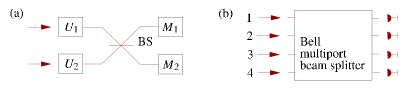
Figure 4: Linear optics networks for the realization of a measurement of the basis states (III.3) after encoding the photonic qubits in the polarization degrees of two photons (a) or into four different spatial photon modes (b) involving either a beam splitter or a $4\times 4$ Bell multiport beam splitter.

Any unknown fixed (or slowly varying with respect to the coherence length of the photon pulse) phase factor introduced along the photon paths contributes at most to a global phase factor to the input state (7), which is also a feature of the schemes outlined in Refs. last ; Simon ; lim ; moonlight . The implementation of Repeat-Until-Success quantum computing therefore does not require interferometric stability. It requires only overlapping of the photons within their coherence length within the linear optics setup.

V Scalable quantum computation in the presence of inefficient photon generation and detection

In this section, we discuss the possibility of implementing scalable quantum computation using the Repeat-Until-Success quantum gate described in the previous sections. The implementation of this gate requires the generation of single photons on demand and linear optical elements together with absorbing quantum measurements. In the limit of perfect photon emission, collection, and detection efficiency, two-qubit CZ gates can be performed deterministically, as described above. In real systems however, photon emission, collection, and detection is not perfect kok01 . In existing experiments, all of these processes have significant inefficiencies, which means that there is a finite probability that two photons will not be observed in the photon measurement. The failure to observe two photons in an attempted CZ operation means that the static qubits are left in an unknown state, which constitutes a correlated two qubit error. If such losses are sufficiently small (e.g. less than $\sim 10^{-2}$), the resulting gate failures can be dealt with using existing fault tolerance techniques steane2003 ; knill2005 . Recently, much higher fault tolerance levels of up to 50% were found in linear optical quantum computing varnava ; gilchrist .

More concretely, the highest reported photon detection efficiency for single photon detection with photon number resolution is about $88\%$ Takeuchi99 ; Rosenberg . A recent experiment by McKeever et al. Mckeever involving an atom-cavity system for the generation of single photons yields a photon generation efficiency of nearly 70%, limited only by passive cavity loss. The lifetime of the atom in the cavity was $0.14\,$s, allowing for as many as $1.4\cdot 10^{4}$ photon generation events. Moreover, Legero et al. Legero demonstrated perfect time-resolved interference with two photons of different frequencies. Time-resolved detection acts as a temporal filter to erase the which-way information which is important to any scheme involving photon interference. This suggests that strictly identical single photon sources are not required for attaining high fidelities in the state preparation. The cost of this high fidelity is a lower probability of success.

Fortunately, scalable quantum computing is possible, even in the presence of large errors, as long as no errors imply a very high fidelity and the occurrence of an error is heralded: if fewer than two photons are detected, we know that the attempted CZ operation has failed. Only when the detectors have a substantial amount of dark counts, we cannot rely on this error detection mechanism. However, comercially available silicon avalanche photodetectors are available with a detection efficiency of 65%, and a dark count rate of $\Gamma_{dc}\leq 25\,$s^-1 PED . Assuming, a photon regeneration rate of $105\,$s^-1 gives a clock time of $10^{-5}$ s. The total dark count probability is then $p_{dc}\approx 10^{-4}$ per clock cycle, which is small enough to be dealt with using existing error correction techniques. Moreover, if one could experiment with detectors like the one reported by Rosenberg et al. Rosenberg , dark count rate effects would be negligible.

In the case of an error, the state of the static qubits can be determined by subsequently performing measurements on the sources, which allows the sources to be re-prepared in a known state. In earlier work, we have shown that scalable quantum computation can be performed in the presence of significant heralded error rates, by first using a non-deterministic entangling operation to create cluster states of many qubits Sean , and subsequently implementing scalable quantum computation via the ‘one-way quantum computer’ raussendorf . Given cluster states of many qubits, the one-way quantum computer can be implemented by single qubit measurements alone. This technique permits fully scalable quantum computation, albeit with a fixed overhead per two qubit gate in the algorithm, which we calculate below. We briefly review how one way quantum computing can proceed within our scheme, and then provide an estimate of the overhead costs involved.

V.1 One way quantum computation

One way quantum computation raussendorf proceeds by first creating a graph state of many qubits, and subsequently performing single qubit measurements on the graph state rbb ; hein ; weinstein . Graph states may be represented as a graph comprising set of qubit ‘nodes’ connected by ‘edges’ which may be understood as ‘bonds’ between the qubits. The quantum state corresponding to such a graph may be defined (and also implemented) by the following procedure: (i) prepare each qubit in the state $|+\rangle=(|0\rangle+|1\rangle)/\sqrt{2}$, and then (ii) for each bond in the corresponding graph, apply a deterministic CZ operation (see Eq. 24) between the relevant qubits. In this work, we will restrict our attention to the rectangular lattice graph states of the form shown in Figure 5 (hereafter referred to simply as cluster states), which are sufficient for simulating arbitrary logic networks, and hence universal quantum computations nielsen04 . It is worth noting however that straightforward generalizations of the procedure described below allow us to scalably generate arbitrary graph states. This may be useful in that it might result in reduced costs for implementing certain algorithms.

Figure 5: A rectangular lattice cluster state. Each circle represents a physical qubit, and each line represents a ‘bond’ between qubits. These states are sufficient for simulating arbitrary logic networks nielsen04 , with each horizontal row representing a single logical qubit, and each vertical connection representing a two-qubit gate. Note we also permit bonds between non-adjacent rows and columns (not shown), which can simulate non-nearest neighbor two-qubit operations.

In these clusters, each horizontal row of physical qubits represents a single logical qubit in the logic network being simulated. Two qubit operations are implemented by the vertical bonds acting between rows. We also permit bonds between non-adjacent rows, which permits highly non-local two qubit gates to be implemented. Note also that the location of the qubits within the cluster is notional, and need not correspond to the physical location of the static qubit (the mapping between the notional qubit positions within the cluster, and the actual physical location of the qubits can be stored in a classical computer). After making the state, quantum computation proceeds by performing a sequence of single qubit measurements on the static qubits, with each measurement performed in a particular basis so as to implement a given sequence of one- and two-qubit gates raussendorf ; nielsen04 . At each time step, a whole column of physical qubits in the cluster is measured. The measurements are performed in order, starting with the column at left side of the cluster, and proceeding rightwards across the cluster. In general, the basis of the measurements made at a given time step will depend on the outcomes of earlier measurements. Once a physical qubit has been measured, that qubit is disentangled from the cluster state and so may be re-initialized in a particular state and subsequently used later in the computation.

We assume that single-shot single qubit measurements and single qubit unitary operations on the static qubits can be implemented using standard techniques. Implementing one-way quantum computation in our scheme therefore reduces to the problem of scalably generating cluster states using the heralded, non-deterministic CZ operation. We outline the general procedure here, and give a more detailed description in the subsequent section.

In our scheme, cluster states can be generated by attempting to bond qubits using the non-deterministic CZ operation. This operation has three possible outcomes: ‘success’, ‘insurance’, or ‘failure’. In the case of observing two photons, one of the gates of Eq.(III.4) is implemented, and subsequent application of appropriate single qubit unitaries implements either the CZ operation (denoting a ‘success’), or the identity operation (denoting ‘insurance’). In the case of insurance, the CZ operation can simply be reattempted. Observing fewer than two photons denotes a failure. In this case, the static qubits are left in an unknown state. However, this damage can be repaired as follows. Firstly, each of the two qubits involved in the failed gate can be measured in the computational basis to determine the nature of the error. If either qubit was already part of a cluster state, the bonds to its neighbors within the cluster are also destroyed. However, the remainder of the cluster state can be recovered by applying appropriate single qubit unitary operations to these neighboring qubits, conditional on the outcome of the measurement on the qubit involved in the failed CZ gate. Therefore, the cluster state can grow, shrink, or remain the same size, depending whether the CZ operation was successful, failed, or failed with insurance. The key to scalably generating cluster states is to attempt CZ operations between qubits in a sequence order such that the cluster state grows on average. We give such a sequence in Sec. V.2.

Figure 6: Dynamically growing clusters during a computation. The cluster contains three regions: the active region (M), at the left of the cluster, in which the logic gate networks are being simulated via single qubit measurements; the buffer region; and the connection region, where new cluster fragments are added to the right edge of the main cluster. The connecting cluster chains have a buffer length $L_{a}$ to accommodate the probabilistic entangling operation.

We conclude this section by noting that it is not necessary to build the whole cluster required for simulating a particular algorithm before commencing the single qubit measurement part of the computation. It is possible to build a partial cluster, and then to simultaneously perform single qubit measurements on one part of the cluster, while adding new qubits to another region in the cluster. In this approach to one-way quantum computing, one can think of the cluster as being split into three regions, as shown in Figure 6. The active region, to the left of the cluster, contains the part of the cluster where the logic gate networks are being simulated via single qubit measurements. At the right of the cluster, the connection region comprises of several horizontal dangling linear chains which extend from the right edge of the main cluster, each corresponding to a logical qubit. In this region, nondeterministic CZ operations are applied in order to add further cluster sections to the main section. These additional sections are manufactured separately, as described in Sec. V.2. Between the active region and the connection region, the buffer region comprises a quiescent region which suffices to protect the active region in the event of a long sequence of failed CZ operations; this would lead to the right edge of the cluster running back into the active region, damaging the logical computation. The depth of the buffer region should be chosen such that the probability of erasing a logical qubit is sufficiently small that it can be handled with existing fault tolerance techniques steane2003 ; knill2005 .

There are several advantages to this approach. Firstly, fewer physical qubits are needed, because qubits that have already been measured at the left edge of the cluster can be recycled and added to the right hand side of the cluster. Secondly, preparing the whole cluster initially means that some of the qubits will spend a lot of time in an ‘idle’ state before they are involved in the computation; any errors accumulated in these idle qubits due to decoherence will degrade the fidelity of the computation raussendorf . This is crucial if fault tolerant quantum computation is to be implemented within the cluster model, as such schemes require a source of fresh ancilla qubits throughout the algorithm. Thirdly, the overhead costs for this approach can be reduced, because it is not necessary to prepare the whole cluster with a total success probability close to one; the probability for erasing a given logical qubit need only be made smaller than the error threshold required for fault tolerance.

V.2 Overhead costs

A number of authors have considered efficient cluster state generation using non-deterministic, but heralded, Entangling Operations (EOs) yoran03 ; nielsen04 ; browne04 ; Benjamin ; Sean ; DuanRaussendorf ; benjamin04 ; chen . References yoran03 ; nielsen04 ; browne04 calculated explicit costs for making cluster states of optical qubits in the ideal case (i.e. neglecting photon loss). Subsequently, Barrett and Kok Sean showed that, in the case of hybrid matter-optical systems (such as those considered in this work), arbitrarily small EO success probabilities could be tolerated. They provided a ‘divide and conquer’ algorithm for building linear clusters, which has moderate costs even for small success probability. An efficient algorithm for building two dimensional clusters, capable of simulating arbitrary logic networks was also given in Sean . More recently, in Ref. DuanRaussendorf , a similar algorithm for building linear clusters was proposed, which made more use of recycling, and hence has a lower overhead cost. Ref. DuanRaussendorf also gives an alternative algorithm for making 2-dimensional clusters, and explicitly calculates the associated overhead costs. In Ref. benjamin04 , some elegant cost reducing improvements to the scheme proposed in Ref. Sean were suggested, utilizing the redundantly encoded qubits inherent in the original scheme.

In this work, we will combine elements of the approaches taken in Refs. browne04 ; Sean ; DuanRaussendorf to provide a simple upper bound for the scaling costs for building cluster states using our scheme. This estimate is based on an explicit procedure, and we do not claim that it is optimal; an improved algorithm may yield substantially reduced costs. Nevertheless, the procedure given here allows a straightforward calculation of the overhead costs. Despite its apparent similarity to Refs. Sean ; DuanRaussendorf , there is a crucial difference: in the scheme under consideration in this paper, there is the possibility of obtaining the ‘insurance’ outcome. In general, this leads to a reduction in costs relative to schemes in which there is no insurance outcome.

In the presence of imperfect photon emission, detection, and collection, the performance of the CZ operation can be characterized by three probabilities:

• the probability of successfully implementing the CZ operation on the input qubits (up to local operations), $p_{s}$;

• the probability of obtaining the ‘insurance’ outcome in which known local operations are applied to the qubits, $p_{i}$;

• the probability of failure due to failing to emit, collect, or detect one or more photons during the remote gate operation, $p_{f}$.

These probabilities are determined by the physics of the sources and detectors.

Calculating the total cost of growing cluster states can be simplified by noting that, in the case of obtaining the ‘insurance’ outcome, after applying the necessary single qubit corrections, one simply attempts the gate operation again. This process is repeated until a definite outcome (success or failure) is obtained. Thus, we can define total success and failure probabilities, $P_{s}$ and $P_{f}$, of the corresponding definite outcomes after an (arbitrarily long) sequence of ‘insurance’ outcomes. These probabilities are given by $P_{s}=\sum_{j=0}^{\infty}p_{i}^{j}p_{s}=p_{s}/(1-p_{i})$ and $P_{f}=\sum_{j=0}^{\infty}p_{i}^{j}p_{f}=p_{f}/(1-p_{i})$. The average number of attempted CZ operations required before we obtain a definite outcome is $N_{\mathrm{av}}=1/(1-p_{i})$.

The overhead cost for making cluster states is then found using similar calculations to those presented in Refs. Sean ; DuanRaussendorf . We first calculate the cost (i.e. the number of attempted CZ operations per qubit in the final cluster) of generating linear clusters. If a CZ gate is repeatedly applied between the end qubits of two linear chains, each of length $L_{k}$, either the gate is (ultimately) successful, in which case the total length of the new cluster is $2L_{k}$, or the gate (ultimately) fails, in which case, the length of the original clusters shrinks by one qubit each. Repeatedly applying this procedure until a successful outcome is obtained (or until both original clusters are destroyed) DuanRaussendorf gives the expected length $L_{k+1}=\sum_{i=0}^{L_{k}}2(L_{k}-i)P_{s}P_{f}^{i}\approx 2L_{k}-2p_{f}/p_{s}$. Denoting the average number of attempts to create a chain of length $L_{k}$ by $N_{k}$, we also have $N_{k+1}=2N_{k}+1/p_{s}$. Solving these recursion relations gives a total cost

$$N(L)=\frac{\left(N_{0}+\frac{1}{p_{s}}\right)\left(L-\frac{2p_{f}}{p_{s}}\right)}{\left(L_{0}-\frac{2p_{f}}{p_{s}}\right)}-\frac{1}{p_{s}},$$ (39)

where $N_{0}$ denotes the cost of growing a short cluster of length $L_{0}$. Note that for the average cluster length to grow on each round of the protocol, we require $L_{1}>L_{0}$, which implies that the length of the short chains should satisfy $L_{0}>2p_{f}/p_{s}$.

Figure 7: Creating vertical bonds. a) We start out with two sufficiently long cluster chains, and we wish to create a vertical bond between the two qubits on the left. b) We apply a $\sigma_{x}$ measurement to the two adjacent qubits and a Hadamard operation $H$ on the next. c) This will result in a redundant encoding of the qubits we wish to bond together. d) Applying the entangling operation to the dangling “cherries” will create the vertical bond. Note that we also removed the qubits in the vertical bond by applying another $\sigma_{x}$ measurement, resulting in another redundant encoding. If this procedure fails, we are left with a shorter chain, and we can try to create a vertical bond again.

Chains of fixed length $L_{0}$ can be grown independently using the probabilistic CZ operation, by joining sub-chains together. Growing these short chains adds a constant overhead cost to the cluster generation process. We use a ‘divide and conquer’ approach to making these short chains Sean ; DuanRaussendorf , in which, on each round of the protocol, we attempt to join equal length pairs of linear clusters using the probabilistic CZ operation. If we obtain the ‘insurance’ outcome on any such attempt, we try the operation again, whereas if we fail, we assume (for ease of calculation) that the short chains are discarded. On the $k$th round of this protocol, the length of the chains is $l_{k}=2^{k}$, and the number of attempted CZ operations is given by the recursion relation $n_{k}=2n_{k-1}/P_{s}+N_{\mathrm{av}}/P_{s}$. Solving these relations gives

$$N_{0}(L_{0})=N_{\mathrm{av}}\sum_{i=1}^{\log_{2}L_{0}}\frac{2^{i-1}}{P_{s}^{i}}\,.$$ (40)

Combining Eq. (40) and Eq. (39), one can calculate the total cost of growing linear clusters for given values of $p_{f}$, $p_{s}$ and $p_{i}$. For instance, taking $p_{f}=0.6$, $p_{i}=p_{s}=0.2$, we require $L_{0}>6$. Taking $L_{0}=2^{3}=8$, the total cost for making a linear cluster of length $L$ is found to be $N(L)=185L-1115$ attempted CZ operations. A moderate increase in success probability can dramatically decrease the cost: taking $p_{f}=0.4$, $p_{i}=p_{s}=0.3$, we require $L_{0}>2.67$, and taking $L_{0}=2^{2}=4$, we find the total cost to be $N(L)=16\frac{2}{3}L-47\frac{7}{9}$. Note that the negative constant term in these expressions is an artefact of joining small numbers of chains together to make an isolated chain of length $L$. This is an ‘edge effect’ which should be neglected when considering the asymptotic cost of making long chains.

Table 1: The average number of entangling operations per vertical bond, given by $N_{\rm bond}=2N(M)+(1-p_{i})/p_{s}$. Here $p_{s}$, $p_{f}$ and $p_{i}$ are the success, failure and insurance probabilities, respectively. $L_{0}=2^{n}$ is the length of the chain that is needed to obey the growth requirement, and $N_{0}$ is the number of EOs needed to achieve this length. $M$ is the average cluster chain consumed by the forging of a vertical bond, and $N(M)$ is the number of EOs needed to achieve this length.

$p_{s}$	$p_{f}$	$p_{i}$	$L_{0}$	$N_{0}\phantom{\frac{1}{2}}$	$M$	$N(M)$	$N_{\rm bond}$
0.2	0.6	0.2	$2^{3}=8$	365	9	$185M$	3334
0.3	0.4	0.3	$2^{2}=4$	18$\frac{8}{9}$	5$\frac{2}{3}$	$16\frac{2}{3}M$	191$\frac{2}{9}$
0.4	0.2	0.4	$2^{1}=2$	2$\frac{1}{2}$	3	$5M$	32$\frac{1}{2}$
0.5	0.5	0	$2^{2}=4$	10	5	$6M$	62

Linear clusters are not sufficient for simulating arbitrary logic networks Nielsen2005 , and therefore it is necessary to generate more general graph states. A variety of techniques for making such states using probabilistic entangling operations have been proposed, which include linking linear clusters using independently prepared ‘I’ shaped clusters Sean , using micro-clusters nielsen04 , using redundantly encoded qubits browne04 , or by making use of ‘+’ shaped clusters DuanRaussendorf . Here, we propose a relatively efficient method for creating vertical bonds between linear cluster chains.

We employ a technique based on that introduced by Browne and Rudolph browne04 , which involves four steps as shown in Figure 7.

1. First, we assume that we have sufficiently long linear cluster chains. These can be produced efficiently in the manner outlined above. In order to establish the amount of resources needed to create a vertical bond, we will count the number of qubits that are utilized on average in this process, as well as the average number of entangling operations.

2. Secondly, we identify the two qubits that we wish to entangle with a vertical bond (in Figure 7 the two left-most qubits). The qubits directly on the right of these qubits are then measured in the $\sigma_{x}$ basis. A Hadamard operation on the third qubit in each chain returns the overal state to a graph state.

3. This will result dangling bonds, or cherries tom hanging from the two qubits that are to be connected. This is a form of redundant encoding, and it allows us to apply the entangling operation to the two cherries. In case of a failure, the entangling operation will not break the linear cluster chains. It will destroy only the cherries and as a result both chains are shortened by two qubits. Steps (b) and (c) can then be repeated.

4. When the entangling operation succeeds, we have forged a vertical bond between the two qubits chosen in step a). The vertical link is itself a chain of two qubits. These are typically not wanted, so we can remove one of them with a $\sigma_{x}$ measurement, creating another cherry in the other qubit in the chain. This redundancy can be pruned, but may also be useful for creating additional bonds, or may even be useful for error correction.

We will now estimate the cost of this procedure. Since two qubits are burnt in each step, and we need to repeat the process $P_{s}^{-1}$ times, the average length of each chain that is consumed in the bonding process is

$$M=2P_{s}^{-1}+1=\frac{2(1-p_{i})}{p_{s}}+1\;,$$ (41)

where the extra $+1$ counts the qubits that will establish the vertical link. The number of entangling operations needed to make a vertical bond is then

$$N_{\rm bond}=2N(M)+P_{s}^{-1}=2N(M)+\frac{(1-p_{i})}{p_{s}}\;,$$ (42)

where the extra $P_{s}^{-1}$ takes into account the number of entangling operations that are needed to link the cherries together into a vertical bond. In Table 1, we calculated the number of entangling operations that are needed to forge a vertical bond, given several specific values for the success, failure, and insurance probabilities.

VI Conclusions

We analysed a hybrid architecture for quantum computing using stationary and flying qubits, which is based on our earlier work moonlight ; Sean , in detail. It was shown that this new approach solves some of the most pressing problems that arise in non-hybrid architectures. Our system is scalable, even with non-ideal components, and more importantly, it uses no direct qubit-qubit interactions. This means that the qubits will be subject to less decoherence and fewer control errors. When realistic photo-detectors are used, photon loss will affect only the efficiency of the scheme. Furthermore, our system relies on components that have been demonstrated in experiment, and is largely implementation independent. Despite the no-go theorem for optical Bell-state measurements, it is in principle possible to implement a deterministic gate between distant qubits.

However, when losses are taken into account, the gate becomes necessarily probabilistic. In order to achieve robustness against general decoherence and to guarantee high fidelities, we showed how to construct cluster- or graph-states using the two-qubit gate. Our entangling operation, which produces the bonds in the graph states, is not limited to physically adjacent matter qubits. As a consequence, no extensive swapping operations need to be taken into account in the production of nontrivial graph states. This architecture for quantum computation is inherently distributed, and hence can be used for integrated quantum computation and communication purposes.

Acknowledgment. YLL, AB and LCK thank H.J. Briegel, A. Browaeys, D.E. Browne, T. Durt, A.K. Ekert, P. Grangier, M. Jones, and P.L. Knight for stimulating discussions. PK and SDB thank S. Benjamin, J. Eisert, B. Lovett, M.A. Nielsen, T. Stace for fruitful discussions and particularly D. Browne for giving them a deeper insight into cluster state generation. YLL acknowledges funding from the DSO National Laboratories in Singapore and AB acknowledges support from the Royal Society and the GCHQ. This work was supported in part by the European Union (RAMBOQ, QGATES) and the UK Engineering and Physical Sciences Research Council (QIP IRC).

References

- (1) P.W. Shor, ed. by S. Goldwasser, Proceedings of the 35th Annual Symposium on the Foundations of Computer Science, IEEE Computer Society, p. 124 (1994).
- (2) D. Deutsch, Proc. R. Soc. A 400, 97 (1985).
- (3) L.M.K. Vandersypen, M. Steffen, G. Breyta, C.S. Yannoni, M.H. Sherwood, and I.L. Chuang, Nature 414, 883 (2001).
- (4) F. Jelezko, T. Gaebel, I. Popa, M. Domhan, A. Gruber, and J. Wrachtrup, Phys. Rev. Lett. 93, 130501 (2004).
- (5) F. Schmidt-Kaler, H. Häffner, M. Riebe, S. Gulde, G.P.T. Lancaster, T. Deuschle, C. Becher, C. F. Roos, J. Eschner, and R. Blatt, Nature 422, 408 (2003).
- (6) D. Leibfried, B. DeMarco, V. Meyer, D. Lucas, M. Barrett, J. Britton, W.M. Itano, B. Jelenkovic, C. Langer, T. Rosenband, and D. J. Wineland, Nature 422, 412 (2003).
- (7) M. Riebe, H. Häffner, C. F. Roos, W. Hansel, J. Benhelm, G.P.T. Lancaster, T.W. Korber, C. Becher, F. Schmidt-Kaler, D.F.V. James, and R. Blatt, Nature 429, 734 (2004).
- (8) J. Chiaverini, D. Leibfried, T. Schaetz, M.D. Barrett, R.B. Blakestad, J. Britton, W.M. Itano, J.D. Jost, E. Knill, C. Langer, R. Ozeri, and D.J. Wineland, Nature 432, 602 (2004).
- (9) D. Kielpinski, C. Monroe, and D.J. Wineland, Nature 417, 709 (2002).
- (10) C.H. Bennett and G. Brassard, Proc. IEEE Int. Conf. Computers, Systems and Signal Processing, Bangalore, India, p. 175 (1984).
- (11) A.K. Ekert, Phys. Rev. Lett. 67, 661 (1991).
- (12) E. Knill, R. Laflamme, and G.J. Milburn, Nature 409, 46 (2001).
- (13) R. Raussendorf and H.J. Briegel, Phys. Rev. Lett. 86, 5188 (2001).
- (14) N. Yoran and B. Reznik, Phys. Rev. Lett. 91, 037903 (2003).
- (15) M.A. Nielsen, Phys. Rev. Lett. 93, 040503 (2004).
- (16) D.E. Browne and T. Rudolph, Phys. Rev. Lett. 95, 010501 (2005).
- (17) P. Walther, K.J. Resch, T. Rudolph, E. Schenck, H. Weinfurter, V. Vedral, M. Aspelmeyer, and A. Zeilinger, Nature 434, 169 (2005).
- (18) R.M. Gingrich, P. Kok, H. Lee, F. Vatan, and J.P. Dowling, Phys. Rev. Lett. 91, 217901 (2003).
- (19) L.K. Grover, Bell Labs Technical Memorandum No. ITD-96-30115J, quant-ph/9607024 (1996).
- (20) J.I. Cirac, A.K. Ekert, S.F. Huelga, and C. Macchiavello, Phys. Rev. A 59, 4249 (1999).
- (21) J. Eisert, K. Jacobs, P. Papadopoulos, and M.B. Plenio, Phys. Rev. A 62, 052317 (2000).
- (22) L.-M. Duan, B.B. Blinov, D.L. Moehring, and C. Monroe, Quant. Inf. Comput. 4, 165 (2004).
- (23) J.M. Taylor, G. Giedke, H. Christ, B. Paredes, J.I. Cirac, P. Zoller, M.D. Lukin, and A. Imamoglu, cond-mat/0407640 (2004).
- (24) J.I. Cirac, P. Zoller, H.J. Kimble, and H. Mabuchi, Phys. Rev. Lett. 78, 3221 (1997).
- (25) S.J. van Enk, J.I. Cirac, and P. Zoller, Phys. Rev. Lett. 78, 4293 (1997).
- (26) A. Sørensen and K. Mølmer, Phys. Rev. A 58, 2745 (1998).
- (27) M.N. Leuenberger, M.E. Flatte, and D.D. Awschalom, cond-mat/0407499 (2004).
- (28) Y.-F. Xiao, X.-M. Lin, J. Gao, Y. Yang, Z.-F. Han, and G.-C. Guo, Phys. Rev. A 70, 042314 (2004).
- (29) X-F. Zhou, Y-S. Zhang, and G.-C. Guo, Phys. Rev. A 71, 064302 (2005).
- (30) S. Mancini and S. Bose, Phys. Rev. A 70, 022307 (2004).
- (31) J.D. Franson, B.C. Jacobs, and T.B. Pittman, Phys. Rev. A 70, 062302 (2004).
- (32) S.D. Barrett, P. Kok, K. Nemoto, R.G. Beausoleil, W.J. Munro, and T.P. Spiller, Phys. Rev. A 71 060302(R) (2005).
- (33) C. Cabrillo, J.I. Cirac, P. Garcia-Fernandez, and P. Zoller, Phys. Rev. A 59, 1025 (1999).
- (34) S. Bose, P.L. Knight, M.B. Plenio, and V. Vedral, Phys. Rev. Lett. 83, 5158 (1999).
- (35) L.M. Duan, M.D. Lukin, J.I. Cirac, and P. Zoller, Nature 414, 413 (2001).
- (36) L.-M. Duan and H. J. Kimble, Phys. Rev. Lett. 90, 253601 (2003).
- (37) D.E. Browne, M.B. Plenio, and S.F. Huelga, Phys. Rev. Lett. 91, 067901 (2003).
- (38) C. Simon and W.T.M. Irvine, Phys. Rev. Lett. 91, 110405 (2003).
- (39) Y.L. Lim and A. Beige, J. Phys. A 38, L7 (2005).
- (40) X.B. Zou and W. Mathis, Phys. Rev. A 71, 042334 (2005).
- (41) G. Chimczak, R. Tanas, and A. Miranowicz, Phys. Rev. A 71, 032316 (2005).
- (42) I.E. Protsenko, G. Reymond, N. Schlosser, and P. Grangier, Phys. Rev. A 66, 062306 (2002); N. Schlosser, I.E. Protsenko, and P. Grangier, Phil. Trans. Roy. Soc. Lond. A 361, 1527 (2003).
- (43) Y.L. Lim, A. Beige, and L.C. Kwek, Phys. Rev. Lett. 95, 030505 (2005).
- (44) S.D. Barrett and P. Kok, Phys. Rev. A 71, 060310(R) (2005).
- (45) B.B. Blinov, D.L. Moehring, L.-M. Duan, and C. Monroe, Nature 428, 153 (2004).
- (46) M. Weber, PhD Thesis, Ludwig-Maximilian-Universität München (2005).
- (47) M. Hennrich, T. Legero, A. Kuhn, and G. Rempe, Phys. Rev. Lett. 85, 4872 (2000); A. Kuhn, M. Hennrich and G. Rempe, Phys. Rev. Lett. 89, 067901 (2002).
- (48) O. Benson, C. Santori, M. Pelton, and Y. Yamamoto, Phys. Rev. Lett. 84, 2513 (2000); M. Pelton, C. Santori, J. Vuckovic, B. Zhang, G.S. Solomon, J. Plant, and Y. Yamamoto, Phys. Rev. Lett 89, 233602 (2002).
- (49) J. McKeever, A. Boca, A. D. Boozer, R. Miller, J. R. Buck, A. Kuzmich and H. J. Kimble, Science 303, 1992 (2004).
- (50) M. Keller, B. Lange, K. Hayasaka, W. Lange, and H. Walther, Nature 431, 1075 (2004).
- (51) D.N. Matsukevich and A. Kuzmich, Sience 306, 663 (2004).
- (52) B. Darquie, M.P.A. Jones, J. Dingjan, J. Beugnon, S. Bargamini, Y. Sortais, G. Messin, A. Browaeys, and P. Grangier, Science 309, 454 (2005).
- (53) D. Rosenberg, A.E. Lita, A.J. Miller, and S.W. Nam, Phys. Rev. A 71, 061803(R) (2005).
- (54) D. Gottesman, J. Mod. Opt. 47, 333 (2000).
- (55) W.K. Wootters and B.D. Fields, Annals of Physics, 191, 363 (1989).
- (56) D. Gottesman and I.L. Chuang, Nature 402, 390 (1999).
- (57) M.A. Nielsen, Phys. Lett. A 308, 96 (2003).
- (58) A.M. Childs, D.W. Leung, and M.A. Nielsen, Phys. Rev. A 71, 032318 (2005).
- (59) A. Beige, D. Braun, B. Tregenna, and P. L. Knight, Phys. Rev. Lett. 85, 1762 (2000).
- (60) A. Beige, Phys. Rev. A 69, 012303 (2004).
- (61) G.G. Lapaire, P. Kok, J.P. Dowling, and J.E. Sipe, Phys. Rev. A 68, 042314 (2003).
- (62) D. DiVincenzo, in Scalable quantum computers; paving the way to realization, S.L. Braunstein and H.-K. Lo (Eds.) Wiley-VCH, Berlin (2001).
- (63) This gate can be easily accomplished by applying a strongly detuned laser field for a certain time .
- (64) L. Vaidman and N. Yoran, Phys. Rev. A 59, 116 (1999); N. Lütkenhaus, J. Calsamiglia, and K. A. Suominen, Phys. Rev. A 59, 3295 (1999).
- (65) K.M. Gheri, C. Saavedra, P. Törmä, J. I. Cirac, and P. Zoller, Phys. Rev. A 58, R2627 (1998).
- (66) C.K. Law and H.J. Kimble, J. Mod. Opt. 44, 2027 (1997); A. Kuhn, M. Hennrich, T. Bondo, and G. Rempe, Appl. Phys. B 69, 373 (1999).
- (67) M. Zukowski, A. Zeilinger, and M.A. Horne, Phys. Rev. A 55, 2564 (1997).
- (68) P. Kok and S.L. Braunstein, Phys. Rev. A 63, 033812 (2001).
- (69) A. M. Steane, Phys. Rev. A 68, 042322 (2003).
- (70) E. Knill, Nature 434, 39 (2005).
- (71) M. Varnava, D.E. Browne, and T. Rudolph, quant-ph/0507036 (2005).
- (72) T.C. Ralph, A.J.F. Hayes, and A. Gilchrist, Phys. Rev. Lett. 95, 100501 (2005).
- (73) S. Takeuchi, J. Kim, Y. Yamamoto and H. H. Hoguer, Appl. Phys. Lett. 74, 1063 (1999).
- (74) T. Legero, T. Wilk, M. Hennrich, G. Rempe and A. Kuhn, Phys. Rev. Lett. 93, 070503 (2004).
- (75) Perkin-Elmer data sheet, available at http://optoelectronics.perkinelmer.com/content/ Datasheets/SPCM-AQR.pdf.
- (76) R. Raussendorf, D.E. Browne, and H. J. Briegel, Phys. Rev. A 68, 022312 (2003).
- (77) M. Hein, J. Eisert, and H.J. Briegel, Phys. Rev. A 69, 062311 (2004).
- (78) Y.S. Weinstein, C.S. Hellberg, and J. Levy, Phys. Rev. A 72, 020304(R) (2005).
- (79) L.-M. Duan and R. Raussendorf, Phys. Rev. Lett. 95, 080503 (2005).
- (80) S.C. Benjamin, quant-ph/0504111 (2005).
- (81) S.C. Benjamin, J. Eisert, and T. Stace, new J. Phys. 7, 194 (2005).
- (82) Q. Chen, J. Cheng, K.-L. Wang, and J. Du, quant-ph/0507066 (2004).
- (83) M. A. Nielsen, Rev. Math. Phys. (in press); quant-ph/0504097 (2005).
- (84) Terminology introduced by T.M. Stace.