Entanglement properties in (1/2,1) mixed-spin Heisenberg systems

Abstract

By using the concept of negativity, we investigate entanglement in (1/2,1) mixed-spin Heisenberg systems. We obtain the analytical results of entanglement in small isotropic Heisenberg clusters with only nearest-neighbor (NN) interactions up to four spins and in the four-spin Heisenberg model with both NN and next-nearest-neighbor (NNN) interactions. For more spins, we numerically study effects of temperature, magnetic fields, and NNN interactions on entanglement. We study in detail the threshold value of the temperature, after which the negativity vanishes.

I Introduction

Entanglement, an essential feature of the quantum mechanics, has been introduced in many fields of physics. In the field of quantum information, the entanglement has played a key role. The study of entanglement properties in many-body systems have attracted much attention M_Nielsen -QPT_GVidal . The Heisenberg chains, widely studied in the condensed matter field, display rich entanglement features and have many useful applications such as in the quantum state transfer M_Sub .

Most of the systems considered in previous studies are spin-half systems as there exists a good measure of entanglement of two spin-halves, the concurrence Conc , which is applicable to an arbitrary state of two spin halves. On the other hand, the entanglements in mixed-spin or higher spin systems are not well-studied due to the lack of good operational entanglement measures. There are several initial studies along this direction Schliemann ; Yi ; Zhu , however these works are restricted to the case of two particles.

For the case of higher spins, a non-entangled state has necessarily a positive partial transpose according to the Peres-Horodecki criterion PH . In the case of two spin halves, and the case of (1/2,1) mixed spins, fortunately, a positive partial transpose is also sufficient. Thus, the sufficient and necessary condition for entangled state in (1/2,1) mixed spin systems is that it has a negative partial transpose. This allows us to investigate entanglement features of the mixed spin system.

The Peres-Horodecki criterion give a qualitative way for judging whether the state is entangled or not. The quantitative version of the criterion was developed by Vidal and Werner Vidal . They presented a measure of entanglement called negativity that can be computed efficiently, and the negativity does not increase under local manipulations of the system. The negativity of a state $\rho$ is defined as

$${\cal N(\rho)}=\sum_{i}|\mu_{i}|,$$ (1)

where $\mu_{i}$ is the negative eigenvalue of $\rho^{T_{1}}$, and $T_{1}$ denotes
the partial transpose with respect to the first system. The negativity ${\cal N}$ is related to the trace norm of $\rho^{T_{1}}$ via

$${\cal N(\rho)}=\frac{\|\rho^{T_{1}}\|_{1}-1}{2},$$ (2)

where the trace norm of $\rho^{T_{1}}$ is equal to the sum of the absolute values of the eigenvalues of $\rho^{T_{1}}$. In this paper, we will use the concept of negativity to study entanglement in (1/2,1) mixed-spin systems.

As shown in most previous works, models with the NN exchange interactions are considered and it is not easy to have pairwise entanglement between the NNN spins M_Osborne ; M_Osterloh . It is true that there exist some quasi-one-dimension compounds offering us systems with NNN interactions. Bose and Chattopadhyay Ibose and Gu et al. Gu have investigated entanglement in spin-half Heisenberg chain with NNN interactions. In our paper here, we study entanglement properties not only in the (1/2,1) mixed-spin systems only with NN interactions, but also in the system with NNN interactions.

Entanglement in a system with a few spins displays general features of entanglement with more spins. For instance, in the anisotropic Heisenberg model with a large number of qubits, the pairwise entanglement shows a maximum at the isotropic point Gu . This feature was already shown in a small system with four or five qubits Wang04 . So, the study of small systems is meaningful in the study of entanglement as they may reflect general features of larger or macroscopic systems. Also, due to the limitation of our computation capability, we only concentrate on small systems such as 4, 5 and 6-spin models.

The paper is organized as follows. In Sec. II, we study the systems with only NN interactions. The analytical results of negativity for the cases of two and three spins are given. The relation between entanglement and the macroscopic thermodynamical function, the internal energy is revealed. Also we numerically compute the negativity in more general mixed-spin models up to eight spins, and consider the effects of magnetic fields in this section. In Sec. III, the system with NNN interaction is discussed. For the four-spin case, we analytically calculate the eigenenergy of the system from which we get the analytical results of the negativity of the NN spins. We numerically study negativities versus NNN exchanging coupling, and the case of finite temperature is also considered. For larger system up to eight-spin system, we get some numerical results. The conclusion is given in Sec. IV.

II Entanglement in Heisenberg chain only with nearest-neighbor interaction

II.1 Analytical results of Entanglement in Heisenberg models

We study entanglement of states of the system at thermal equilibrium described by the density operator $\rho(T)=\exp(-\beta H)/Z$, where $\beta=1/k_{B}T$, $k_{B}$ is the Boltzmann’s constant, which is assumed to be one throughout the paper , and $Z=\text{Tr}\{\exp(-\beta H)\}$ is the partition function. The entanglement in the thermal state is called thermal entanglement.

We consider two kinds of spins, spin $\frac{1}{2}$ and $1$, alternating on a ring with antiferromagnetic exchange coupling. The Hamiltonian is given by

$$H_{0} = \sum_{i=1}^{N/2}({\bf s}_{i}\cdot{\bf S}_{i}+{\bf S}_{i}\cdot{\bf s}_{i+1}),(N\in\text{even})$$ (3)

$$H_{0} = \sum_{i=1}^{(N-1)/2}({\bf s}_{i}\cdot{\bf S}_{i}+{\bf S}_{i}\cdot{\bf s}_{i+1})+{\bf s}_{\frac{(N+1)}{2}}\cdot{\bf s}_{1},$$ (4)

$$(N\in\text{odd}),$$

where ${\bf s}_{i}$ and ${\bf S}_{i}$ are spin-1/2 and spin-1 operators, respectively. The exchange interactions exist only between nearest neighbors, and they are of the same strength which are set to one. We adopt the periodic boundary condition. In Fig. 1, we give the schematic representation of the above Hamiltonian. Next, we first consider the models with two and three spins, and aim at getting analytical results of entanglement.

II.1.1 Two-spin case

For the two-spin case, the Hamiltonian (3) reduces to $H_{0}={\bf s}_{1}\cdot{\bf S}_{1}$. To have a matrix representation of the Hamiltonian, we choose the following basis

$$\Big{\{}|-\frac{1}{2},-1\rangle,|\frac{1}{2},0\rangle,|-\frac{1}{2},1\rangle,|\frac{1}{2},-1\rangle,|-\frac{1}{2},0\rangle,|\frac{1}{2},1\rangle\Big{\}},$$ (5)

where $|m,M\rangle$ is the eigenstate of ${s}_{z}$ and $S_{z}$ with the corresponding eigenvalues given by $m$ and $M$, respectively.

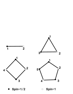
Figure 1: Schematic representation of the mixed spin Hamiltonian for the number of spins from 2 to 5.

In the above basis, the Hamiltonian can be written as a block-diagonal form with the dimension of each block being at most $2\times 2$. Thus, the density matrix $\rho_{12}$ for the thermal state is obtained as

$$\rho_{12}=\left(\begin{array}[]{llllll}a_{1}&0&0&0&0&0\\ 0&a_{2}&b_{1}&0&0&0\\ 0&b_{1}&a_{3}&0&0&0\\ 0&0&0&a_{4}&b_{2}&0\\ 0&0&0&b_{2}&a_{5}&0\\ 0&0&0&0&0&a_{6}\end{array}\right),$$ (6)

with the partition function and the matrix elements given by

$$Z = 2e^{\beta}+4e^{-\frac{1}{2}\beta},$$ (7)

$$a_{1} = a_{6}=e^{-\frac{1}{2}\beta}/Z,$$ (8)

$$a_{2} = a_{5}=\frac{1}{6},$$ (9)

$$a_{3} = a_{4}=\frac{1}{3}\left(2e^{\beta}+e^{-\frac{1}{2}\beta}\right)/Z,$$ (10)

$$b_{1} = b_{2}=\frac{\sqrt{2}}{3}\left(e^{-\frac{1}{2}\beta}-e^{\beta}\right)/Z,$$ (11)

$$= \sqrt{2}(a_{1}-a_{2}).$$

After the partial transpose with respect to the first spin-half subsystem, we can get $\rho_{12}^{T_{1}}$

$$\rho_{12}^{T_{1}}=\left(\begin{array}[]{llllll}a_{1}&b_{2}&0&0&0&0\\ b_{2}&a_{2}&0&0&0&0\\ 0&0&a_{3}&0&0&0\\ 0&0&0&a_{4}&0&0\\ 0&0&0&0&a_{5}&b_{1}\\ 0&0&0&0&b_{1}&a_{6}\end{array}\right),$$ (12)

which is still of the block-diagonal form, and computation of its eigenvalues is straightforward. There are only two eigenvalues which are possibly negative. The negativity is thus given by

$${\cal N}(\rho_{12})= \frac{1}{2}\max\big{[}0,\sqrt{(a_{1}-a_{2})^{2}+4b_{2}^{2}}-a_{1}-a_{2})\big{]}$$

$$+ \frac{1}{2}\max\big{[}0,\sqrt{(a_{5}-a_{6})^{2}+4b_{1}^{2}}-a_{5}-a_{6}\big{]}.$$ (13)

Substituting Eqs. (7)–(11) leads to the analytical result of negativity

$${\cal N}(\rho)= \max\big{[}0,\sqrt{(a_{1}-a_{2})^{2}+4b_{2}^{2}}-a_{1}-a_{2})\big{]}$$

$$= 2\max[0,a_{2}-2a_{1}]$$

$$= \frac{1}{3}\max\Big{[}0,\frac{e^{\beta}-4e^{-\frac{1}{2}\beta}}{e^{\beta}+2e^{-\frac{1}{2}\beta}}\Big{]},$$ (14)

where the second equality follows from Eq. (11).

We can see that the negativity is a function of the single parameter $\beta$. In the limit of $T\rightarrow 0$, the negativity becomes 1/3 and the ground state is entangled. From Eq. (14), it is direct to check that the negativity is a monotonically decreasing function when temperature increases. After a certain threshold value of the temperature, the entanglement disappears. This threshold value $T_{\text{th}}$ can be obtained as

$$T_{\text{th}}=3/(4\ln 2)\approx 1.0820.$$ (15)

For a ring of spin-half particles interacting via the Hisenberg Hamiltonian, it was shown that the pairwise thermal entanglement is determined by the internal energy WangPaolo . It is natural to ask if similar relations exist in the present mixed-spin system. The internal energy can be obtained from the partition function as

$$U=-\frac{1}{Z}\frac{\partial Z}{\partial\beta}.$$ (16)

Substituting Eq. (7) into the above equation leads to

$$U=\frac{\displaystyle-e^{\beta}+e^{-\frac{1}{2}\beta}}{\displaystyle e^{\beta}+2e^{-\frac{1}{2}\beta}}.$$ (17)

From Eqs. (14) and (17), we obtain a quantitative relation between the negativity and the internal energy

$${\cal N(\rho)}=\frac{1}{3}\max[0,-1-2U].$$ (18)

The above equation builds a connection between the microscopic entanglement and the macroscopic thermodynamical function, the internal energy. The internal energy completely determine the thermal entanglement. From the equation, we can also read that the thermal state becomes entangled if and only if the internal energy $U<-1/2$. Since $U=\langle H\rangle=\langle\bf s_{1}\cdot\bf S_{1}\rangle$, we have

$${\cal N(\rho)}=\frac{1}{3}\max[0,-1-2\langle\bf s_{1}\cdot\bf S_{1}\rangle],$$ (19)

which is consistent with the result obtained in Ref. Schliemann by the group-theoretical technique.

II.1.2 Three-spin case

We now consider the three-spin case and the schematic representation of the corresponding Hamiltonian is given by Fig. 1. In this situation, there are two types of pairwise entanglement, the entanglement between spin 1/2 and spin 1 and the entanglement between two spin halves.

The eigenvalue problem can be solved analytically, and after tracing out the third spin-half system the reduced density matrix $\rho_{12}$ is still of the same form as in Eq. (6) with matrix elements given by

$$a_{1} = \left(\frac{5}{4}e^{-\frac{5}{4}\beta}+\frac{3}{4}e^{\frac{3}{4}\beta}\right)/Z,$$

$$a_{2} = \left(\frac{5}{6}e^{-\frac{5}{4}\beta}+e^{\frac{3}{4}\beta}+\frac{1}{6}e^{\frac{7}{4}\beta}\right)/Z,$$

$$a_{3} = \left(\frac{5}{12}e^{-\frac{5}{4}\beta}+\frac{5}{4}e^{\frac{3}{4}\beta}+\frac{1}{3}e^{\frac{7}{4}\beta}\right)/Z,$$

$$b_{1} = \left(\frac{5\sqrt{2}}{12}e^{-\frac{5}{4}\beta}-\frac{\sqrt{2}}{4}e^{\frac{3}{4}\beta}-\frac{\sqrt{2}}{6}e^{\frac{7}{4}\beta}\right)/Z,$$

$$Z = 5e^{-\frac{5}{4}\beta}+6e^{\frac{3}{4}\beta}+e^{\frac{7}{4}\beta}.$$ (20)

Substituting the above equations to Eq. (13) leads to the negativity

$${\cal N}(\rho_{12})=\max\Big{[}0,{-\frac{10}{3}e^{-\frac{5}{4}\beta}-e^{\frac{3}{4}\beta}+\frac{1}{3}e^{\frac{7}{4}\beta}}\Big{]}/Z.$$ (21)

It is evident that the negativity becomes 1/3 in the limit of $T\rightarrow 0$. From the expression of the negativity, the threshold value of temperature after which the entanglement vanishes can be estimated as

$$T_{\text{th}}\approx 1/\ln 3.2719\approx 0.7609.$$ (22)

To examine the entanglement between two spin halves, we trace out the spin 1 system and get the reduced density matrix $\rho_{13}$ as follows

$$\rho_{13}=\left(\begin{array}[]{llll}a_{1}&0&0&0\\ 0&a_{2}&b&0\\ 0&b&a_{2}&0\\ 0&0&0&a_{1}\end{array}\right),$$ (23)

with the matrix elements given by

$$a_{1} = \left(\frac{5}{3}e^{-\frac{5}{4}\beta}+e^{\frac{3}{4}\beta}+\frac{1}{3}e^{\frac{7}{4}\beta}\right)/Z$$

$$a_{2} = \left(\frac{5}{6}e^{-\frac{5}{4}\beta}+2e^{\frac{3}{4}\beta}+\frac{1}{6}e^{\frac{7}{4}\beta}\right)/Z$$

$$b = \left(\frac{5}{6}e^{-\frac{5}{4}\beta}-e^{\frac{3}{4}\beta}+\frac{1}{6}e^{\frac{7}{4}\beta}\right)/Z.$$ (24)

After taking the partial transpose, we can get $\rho^{T}_{13}$

$$\rho^{T}_{13}=\left(\begin{array}[]{llll}a_{1}&0&0&b\\ 0&a_{2}&0&0\\ 0&0&a_{2}&0\\ b&0&0&a_{1}\end{array}\right).$$ (25)

Then, the negativity is readily obtained as

$${\cal N}(\rho_{13})=\max[0,|b|-a_{1}].$$ (26)

It is straightforward to check that the negativity is always zero. Or, from another way, all the eigenvalues of the matrix $\rho^{T}_{13}$ are obtained as

$$\lambda_{1} = \left(\frac{5}{2}e^{-\frac{5}{4}\beta}+\frac{1}{2}e^{\frac{7}{4}\beta}\right)/Z,$$

$$\lambda_{2} = \left(\frac{5}{6}e^{-\frac{5}{4}\beta}+2e^{\frac{3}{4}\beta}+\frac{1}{6}e^{\frac{7}{4}\beta}\right)/Z,$$

$$\lambda_{3} = \lambda_{4}=a_{2}.$$ (27)

Obviously the negativity vanishes here, in other words there is no entanglement between the two spin halves.

The ground-state negativity ${\cal N}_{12}={\cal N}(\rho_{12})$=1/3 and ${\cal N}_{13}={\cal N}(\rho_{13})$=0, here ${\cal N}_{12}$ denotes the negativity between the $1_{\text{th}}$ and $2_{\text{th}}$ spin on the chain and ${\cal N}_{13}$ denotes the one between the $1_{\text{th}}$ and $3_{\text{th}}$ spin. The equation above can be obtained from the non-degenerate ground state given by:

$$|\psi_{0}\rangle = \frac{\sqrt{6}}{6}\left(|\frac{1}{2},0,-\frac{1}{2}\rangle+|-\frac{1}{2},0,\frac{1}{2}\rangle\right)$$ (28)

$$- \frac{\sqrt{3}}{3}\left(|\frac{1}{2},-1,\frac{1}{2}\rangle+|-\frac{1}{2},1,-\frac{1}{2}\rangle\right).$$

It is interesting to see that the ground-state entanglement between the spin half and spin 1 in the three-spin case is the same as that in the two-spin case.

Due to the SU(2) symmetry in our system, there are following relations between correlation functions and negativities Schliemann

$${\cal N}_{12}= -\frac{1}{3}-\frac{2}{3}\langle{\bf s}_{1}\cdot{\bf S}_{1}\rangle,$$

$${\cal N}_{23}= -\frac{1}{3}-\frac{2}{3}\langle{\bf S}_{1}\cdot{\bf s}_{2}\rangle,$$

$${\cal N}_{31}= -\frac{1}{4}-\langle{\bf s}_{2}\cdot{\bf s}_{1}\rangle,$$ (29)

where we have removed the max function in the negativity, implying that the negative value of ${\cal N}$ indicates no entanglement. Then, we have the relation between the internal energy and the negativities

$$U= -\frac{5}{4}-{\cal N}_{13}-\frac{3}{2}({\cal N}_{12}+{\cal N}_{23})$$

$$= -\frac{5}{4}-{\cal N}_{13}-{3}{\cal N}_{12}.$$ (30)

The second equality follows from the exchange symmetry, namely, the Hamiltonian is invariant when exchanging two spin halves. So, for the three-spin case, the internal energy is related to two negativities.

To apply the above result, we consider the the ground-state properties ($T=0$). The Hamiltonian can be rewritten as

$$H=\frac{1}{2}[({\bf s}_{1}+{\bf S}_{1}+{\bf s}_{2})^{2}-{\bf s}_{1}^{2}-{\bf S}_{1}^{2}-{\bf s}_{2}^{2}].$$ (31)

Then, by the angular momentum coupling theory, the ground-state energy is obtained as $E_{0}=-7/4$. Substituting the ground-state energy and ${\cal N}_{12}=1/3$ to Eq. (30), we obtain ${\cal N}_{13}=-1/2$, indicating that there exists no entanglement between two spin halves. Next, we consider more general situations, i.e., the case of even $N$ sites.

II.1.3 The case of even $N$ spins

Except for the SU(2) symmetry in the system, there exists exchange symmetry for the case of even spins. For instance, in the four-spin model, the Hamiltonian is invariant when exchanging two spin halves or two spin ones. Thus, for even-spin model, the entanglements between the two nearest-neighbor spins and the correlation functions $\langle{\bf s}_{i}\cdot{\bf S}_{i}\rangle$ are independent on index $i$. Therefore, the internal energy per spin is equal to the correlation function $\langle{\bf s}_{i}\cdot{\bf S}_{i}\rangle$

$$u=U/N=\langle{\bf s}_{1}\cdot{\bf S}_{1}\rangle.$$ (32)

From Eqs. (II.1.2) and (32), we have

$${\cal N}_{12}=-\frac{1}{3}-\frac{2}{3}u.$$ (33)

This equation indicates that for the case of even spins the entanglement between two nearest neighbors is solely determined by the internal energy per spin. And for the case of zero temperature, the entanglement is determined by the ground-state energy. The less the energy, the more the entanglement.

We now apply the above result to the study of ground-state entanglement. We rewrite the four-spin Hamiltonian as follows

$$H=\frac{1}{2}[({\bf s}_{1}+{\bf S}_{1}+{\bf s}_{2}+{\bf S}_{2})^{2}-({\bf s}_{1}+{\bf s}_{2})^{2}-({\bf S}_{1}+{\bf S}_{2})^{2}].$$ (34)

Then, by the angular momentum coupling theory, we obtain the ground-state energy per site $e_{0}=E_{0}/4=-3/4$. Thus, from Eq. (33), we have ${\cal N}_{12}=1/6$. For $N\geq 5$, it is hard to get analytical results. We next numerically calculate the entanglement for the case of more spins, and also consider the effects of magnetic fields.

II.2 Numerical results

Having obtained analytical results of entanglement in the Heisenberg model with a few spins, we now numerically examine the entanglement behaviors in more general Hamiltonian including more spins and magnetic fields.

II.2.1 Entanglement versus temperature

We consider the entanglement versus temperature for different number of spins $N$, and the numerical results are plotted in Fig. 2 and Fig. 3. It is clear to see that the ground state exhibits maximal entanglement, and with the increase of temperature, the entanglement monotonically decreases until it reaches zero. The decrease of entanglement is due to the mixture of less entangled excited states when increasing the temperature. The existence of the threshold temperature is also evident. For the case of even number of sites (Fig. 2), the threshold temperature decreases with the increase of $N$. In contrast to this behavior, for the case of odd number of spins, as seen from Fig. 3, the threshold temperature increases with the increase of $N$.

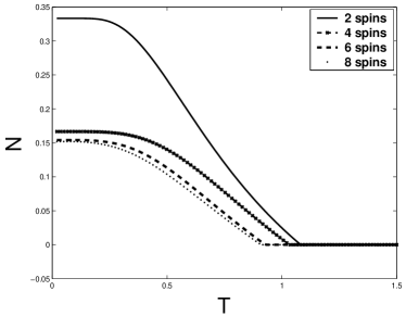
Figure 2: Negativity versus temperature for different even number of spins in the Heisenberg model.

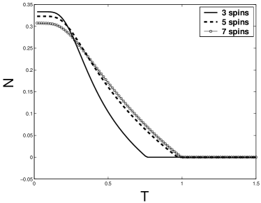
Figure 3: Negativity versus temperature for different odd number of spins in the Heisenberg model.

II.2.2 Effects of magnetic fields

We now examine the effect of magnetic fields on entanglement. The Heisenberg Hamiltonian with a magnetic field along $z$ direction is given by

$$H_{1}=H_{0}+B\sum_{i=1}^{N/2}\big{(}{s}_{iz}+{S}_{i,z}\big{)},(N\in\text{even}).$$ (35)

For $N=2$, the analytical result of negativity can be obtained (see Appendix A).

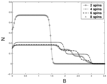
Figure 4: Negativity versus the magnetic field for $T=0.05$.

In Fig. 4, we plot the negativity versus the magnetic field at a low temperature. For the two-spin case, with the increase of the magnetic field, the negativity rapidly reach a platform, and then after a certain magnetic field $B_{\text{th}}$, it jumps down to zero, indicating no entanglement. When $B=0$, the ground state is two-fold degenerate with ${\cal N}=1/3$. For a small $B>0$, the system is no longer degenerate, and the ground state is given by

$$|\psi_{0}\rangle=\frac{\sqrt{6}}{3}|\frac{1}{2},-1\rangle-\frac{\sqrt{3}}{3}|-\frac{1}{2},0\rangle,$$ (36)

which is of the Schmidt form. For a state written as its Schmidt form

$$|\psi\rangle=\sum_{n}c_{n}|e_{n}\rangle|f_{n}\rangle,$$ (37)

the negativity is obtained as Vidal

$${\cal N}=\left[\big{(}\sum_{n}c_{n}\big{)}^{2}-1\right]/2.$$ (38)

Here, $C_{n}$ are the Schmidt coefficients, and $\{|e_{n}\rangle\}$ and $\{|f_{n}\rangle\}$ are bases for subsystems 1 and 2, respectively. Applying this formula to the ground state, we immediately have ${\cal N}=\sqrt{2}/3$. When $B=B_{\text{th}}=3/2$, the ground state is two-fold degenerate, and when $B>B_{\text{th}}$ the ground state becomes non-degenerate and the corresponding wave function is given by

$$|\psi_{0}\rangle=|-\frac{1}{2},-1\rangle,$$ (39)

which is obviously of no entanglement. Then, the ground-state negativity forms a platform when $0<B<B_{\text{th}}$. The jump of negativity at $B=B_{\text{th}}$ is due to the level crossing. For $N>2$, the effects of magnetic fields on entanglement can be also explained by level crossing. For instance, for $N=4$, there are two level crossing, and the entanglement displays two jumps.

III Effects of next-nearest-neighbor interactions on entanglement

We have studied the effects of finite temperature and magnetic fields on entanglement, and now consider the model containing two kinds of spins, spin $\frac{1}{2}$ and $1$, alternating on a ring with antiferromagnetic exchange coupling between both the NN spins and the NNN spins. The Hamiltonian can be expressed as

$$H=J_{1}\sum^{N/2}_{i=1}\big{(}{\bf s}_{i}\cdot{\bf S}_{i}+{\bf S}_{i}\cdot{\bf s}_{i+1}\big{)}+J_{2}\sum^{N/2}_{i=1}\big{(}{\bf s}_{i}\cdot{\bf s}_{i+1}+{\bf S}_{i}\cdot{\bf S}_{i+1}\big{)},$$ (40)

where the ${\bf s}_{i}$ and ${\bf S}_{i}$ are spin-1/2 and spin-1 operators in the $i$th cell. $J_{1}$ characterizes the NN exchange coupling and $J_{2}$ the NNN coupling. We consider the antiferromagnetic interaction by taking $J_{1},J_{2}>0$. $N$ is the total number of spins and here we choose it be even. Also we adopt the periodic boundary condition.

III.1 Four-spin model

III.1.1 Eigenenergy and ground-state entanglement

The model with four spins is the simplest model with NNN interactions. We first solve the eigenvalue problem of this model. The key step is to write the four-spin Hamiltonian in the following form,

$$H = \frac{1}{2}\big{\{}J_{1}{\bf S}^{2}+(2J_{2}-J_{1})[({\bf s}_{1}+{\bf s}_{2})^{2}+({\bf S}_{1}+{\bf S}_{2})^{2}]$$ (41)

$$- 2J_{2}({\bf s}_{1}^{2}+{\bf s}_{2}^{2}+{\bf S}_{1}^{2}+{\bf S}_{2}^{2})\big{\}},$$

where ${\bf S}={\bf S}_{1}+{\bf S}_{2}+{\bf s}_{1}+{\bf s}_{2}$ denotes the total spin. From the above form, by angular momentum coupling theory, one can readily obtain all eigenvalues of the system as

$$E_{1} = J_{2}n(n+1)-\frac{11}{2}J_{2},$$

$$E_{2} = nJ_{1}+n(n+1)J_{2}-\frac{7}{2}J_{2},$$

$$E_{3} = -J_{1}+n(n+1)J_{2}-\frac{7}{2}J_{2},$$

$$E_{4} = -(n+1)J_{1}+n(n+1)J_{2}-\frac{7}{2}J_{2},$$ (42)

where parameter $n=0,1,2$ in expressions $E_{1}$ and $E_{2}$ and $n=1,2$ in expressions $E_{3}$ and $E_{4}$, respectively. Then, from Eq. (42), we may find the ground-state energy as

$$E_{\text{GS}}=\left\{\begin{array}[]{ll}-3J_{1}+\frac{5}{2}J_{2}&\;\text{when}\;\;\;0\leq J_{2}<J_{1}/4,\\ -2J_{1}-\frac{3}{2}J_{2}&\;\text{when}\;\;\;J_{1}/4<J_{2}<J_{1}/2,\\ -\frac{11}{2}J_{2}&\;\text{when}\;\;\;J_{2}>J_{1}/2,\end{array}\right.$$ (43)

Clearly, there are two level-crossing points, which will greatly affect behaviors of ground-state entanglement.

From Eq. (41), it is obvious that in addition to the the SU$(2)$ symmetry, there also exists an exchange symmetry, namely, exchanging two spin halves or two spin ones yields invariant Hamiltonian. Then, the correlator $\langle{\bf s}_{i}\cdot{\bf S}_{i}\rangle$ between any NN spins are the same. Therefore, we can get the correlator $\langle{\bf s}_{i}\cdot{\bf S}_{i}\rangle$ from the ground-state energy via the Hellmann-Feynman theorem.

When $0\leq J_{2}<J_{1}/4$, after applying the Hellmann-Feynman theorem to the ground-state energy, we obtain

$$\langle{\bf s}_{1}\cdot{\bf S}_{1}\rangle=\frac{1}{4}\frac{\partial E_{0}}{\partial J_{1}}=-\frac{3}{4}.$$ (44)

Due to the SU$(2)$ symmetry in our system, we have the following relation between the negativity and the correlator $\langle{\bf s}_{1}\cdot{\bf S}_{1}\rangle$Schliemann ,

$${\cal N}_{1/2,1}=\max\big{\{}0,-\frac{1}{3}-\frac{2}{3}\langle{\bf s}_{1}\cdot{\bf S}_{1}\rangle\big{\}},$$ (45)

where we use ${\cal N}_{1/2,1}$ to denote the negativity between the NN spins. Thus we obtain

$${\cal N}_{1/2,1}=1/6.$$ (46)

In other regions, we find that ${\cal N}_{1/2,1}=0$ for $J_{2}>J_{1}/4$.

From the above analytical results, we can find that the negativity between the NN spins is not a continuous function of parameter $J_{2}$. It jumps from the value $\frac{1}{6}$ down to zero at $J_{2}=0.25$. Hence, we can see that the NNN interaction may deteriorate the entanglement of the NN spins. The critical point of $J_{2}=0.25$ may be considered to be a threshold value, after which the NN entanglement vanishes.

Having studied ground-state entanglement, now we make a short discussion of entanglement of excited states. We consider the first excited state. In the region $J_{1}/4<J_{2}<3J_{1}/8$, the first excited energy is given by

$$E_{1}=-3J_{1}+\frac{5}{2}J_{2},$$ (47)

from that we can get $\langle{\bf s}_{1}\cdot{\bf S}_{1}\rangle=-3/4$ and $N_{1/2,1}=1/6$. While in the rest region the negativity of the first excited state is zero.

III.1.2 Thermal entanglement

Next, we consider the thermal entanglement. From Eq. (42), the partition function can be obtained as

$$Z = 5e^{-\frac{1}{2}\beta J_{2}}+6e^{\frac{7}{2}\beta J_{2}}+e^{\frac{11}{2}\beta J_{2}}$$ (48)

$$+ e^{-\frac{5}{2}\beta J_{2}}(7e^{-2\beta J_{1}}+5e^{\beta J_{1}}+3e^{3\beta J_{1}})$$

$$+ e^{\frac{3}{2}\beta J_{2}}(5e^{-\beta J_{1}}+3e^{\beta J_{1}}+e^{2\beta J_{1}}),$$

The correlator $\langle{\bf s_{1}}\cdot{\bf S_{1}}\rangle$ at finite temperature can be computed from the partition function via the following relation

$$\langle{\bf s_{1}}\cdot{\bf S_{1}}\rangle=-\frac{1}{4\beta Z}\frac{\partial Z}{\partial J_{1}},$$ (49)

Substituting (48) to Eq. (49) yields

$$\langle{\bf s_{1}}\cdot{\bf S_{1}}\rangle = -\frac{1}{4Z}\big{[}e^{-\frac{5}{2}\beta J_{2}}(-14e^{-2\beta J_{1}}+5e^{\beta J_{1}}+9e^{3\beta J_{1}})$$ (50)

$$+ e^{\frac{3}{2}\beta J_{2}}(-5e^{-\beta J_{1}}+3e^{\beta J_{1}}+2e^{2\beta J_{1}})\big{]}.$$

After substituting the above equation into (45), we may get analytical expression of the negativity ${\cal N}_{1/2,1}$ at finite temperatures. The negativity is a function of $J_{1}$, $J_{2}$ and $T$.

Low-temperature case:

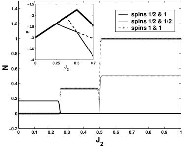
Figure 5: Negativity versus the exchange interaction $J_{2}$ at the temperature $T=0.008$ in the four-spin system. The ground-state and the first two excited-state energy levels versus $J_{2}$ are inserted.

We now make numerical calculations of entanglement and first consider the low-temperature case. We take $J_{1}=1$ in all the following plots. In our system there exist three kinds of negativity, the negativity ${\cal N}_{1/2,1}$ between spin-1 and spin-1/2, ${\cal N}_{1/2,1/2}$ between two spin-1/2, and ${\cal N}_{1,1}$ between two spin-1.

In Fig. 5, we plot the negativity versus $J_{2}$ in four-spin system at a low temperature of $T=0.008$. It is clear to see that ${\cal N}_{1/2,1}$ keeps a value about $1/6$ when $J_{2}$ increases from zero until it reaches the critical point, at which the ${\cal N}_{1/2,1}$ displays a jump to zero. This behavior of entanglement is consistent with that at zero temperature from the analytical results. It is natural to see that increase of NNN exchange interaction will suppress the entanglement of NN spins, and at last completely erase the entanglement.

In comparison with ${\cal N}_{1/2,1}$, the negativities ${\cal N}_{1,1}$ and ${\cal N}_{1/2,1/2}$ behave distinctly. We see that near the point of $J_{2}=1/4$, ${\cal N}_{1,1}$ increases quickly to a steady value about $1/3$, and when $J_{2}$ reaches the value about $1/2$, ${\cal N}_{1,1}$ jumps another steady value 1. These two jumps result from the two level crossing as seen clearly from the figure inserted. The second level crossing also leads to a small dip in the curve of ${\cal N}_{1,1}$. The negativity ${\cal N}_{1/2,1/2}$ displays a jump to a steady value of 1/2 near $J_{2}=1/2$. It is evident that the entanglement between NNN spins is enhanced by increasing NNN interactions. The competition between NN and NNN interactions leads to rich behaviors of quantum entanglement. Another observation is that there is a range of $J_{2}$, at which negativities ${\cal N}_{1/2,1}$ and ${\cal N}_{1/2,1/2}$ are zero, and only ${\cal N}_{1,1}$ is not zero. This indicates that the NNN interaction must be strong enough to build up the entanglement of two spin halves.

Entanglement versus $J_{2}$ and $T$: As temperature increases the entanglement will decrease due to the mixing of less entangled excited states to the thermal state. It is obvious that there exists a threshold temperature after which the negativity is zero. In the frustrated system, there exists the parameter $J_{2}$, and with its increase, the negativity ${\cal N}_{1/2,1}$ will decrease to zero, while ${\cal N}_{1,1}$ and ${\cal N}_{1/2,1/2}$ increase from zero to their maxima. So it is clear that there also exists a threshold $J_{\text{2th}}$ corresponding to the boundary between zero and nonzero negativities.

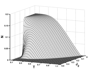
Figure 6: Negativity ${\cal N}_{1/2,1}$ versus both the exchange interaction coefficient $J_{2}$ and the temperature in the four-spin system.

In Fig. 6, we show the negativity ${\cal N}_{1/2,1}$ versus the temperature and $J_{2}$. When the temperature approaches zero, the ${\cal N}_{1/2,1}$ reaches its maximum, and then with the temperature increasing, ${\cal N}_{1/2,1}$ decreases to zero. On the $J_{2}-T$ plane, there is a curve along which the negativity just turns to be zero. It is possible to consider that the curve describes the threshold $J_{\text{2th}}$ versus the temperature. Obviously, $J_{\text{2th}}$ does not behave as a monotonous function of the temperature, and it displays a peak at about $T=0.178$, This behavior is in big contrast with the case of non-mixed qubit systems Gu . When the temperature rises, the weight of excited states will increase and it may strongly affect the negativity. This behavior of $J_{\text{2th}}$ results from both the mixture of excited states to the thermal state and the intrinsic properties of the mixed-spin system. In addition, after crossing the temperature about $T=1.082$, ${\cal N}_{1/2,1}$ will vanish, irrespective of the value of $J_{2}$.

From another point of view, we can read the threshold temperature $T_{\text{th}}$ versus different $J_{2}$ from the curve in the $J_{2}-T$ plane. When $J_{2}$ increases, $T_{\text{th}}$ decreases, and when $J_{2}$ crosses about $0.3758$, ${\cal N}_{1/2,1}$ will disappear at any temperature.

Next, we consider the entanglement between NNN spins. In Fig. 7, we plot the negativity ${\cal N}_{1/2,1/2}$ as a function of the temperature and $J_{2}$. We can see that, before $J_{2}$ reaches the value about $J_{2}=0.5$, ${\cal N}_{1/2,1/2}$ keeps being zero at any temperature. And in the region $J_{2}>0.5$, the ${\cal N}_{1/2,1/2}$ can be enhanced by the increasing NNN interaction. This is a result from the competition of two kinds of exchange interactions. The thermal fluctuation all along suppresses the entanglement. So, from the curve lying on the $J_{2}-T$ plane which corresponds to the boundary of the nonzero and zero values of ${\cal N}_{1/2,1/2}$, we may find that the higher the temperature is, the larger the threshold $J_{\text{2th}}$ will be. From another point of view, the $T_{\text{th}}$ increases as $J_{2}$ increases.

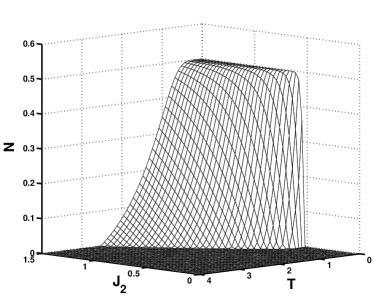
Figure 7: Negativity ${\cal N}_{1/2,1/2}$ versus both the exchange interaction coefficient $J_{2}$ and the temperature in four-spin system.

In Fig. 8, we plot the negativity ${\cal N}_{1,1}$ versus $T$ and $J_{2}$. In the region of $J_{2}<0.25$, ${\cal N}_{1,1}$ is zero at any temperature. When $J_{2}>0.25$, the increasing NNN exchange interaction $J_{2}$ enhances the negativity and exhibits two particular flat roofs. With the temperature rises, ${\cal N}_{1,1}$ is suppressed to zero. Also we can consider the threshold $T_{\text{th}}$ and $J_{\text{2th}}$ from the critical curve on the $J_{2}-T$ plane, and the $J_{\text{2th}}$ also behaves as an increasing function of the temperature. We can see the nonzero region of ${\cal N}_{1,1}$ is much larger than ${\cal N}_{1/2,1/2}$. But here it should be pointed out that, because ${\cal N}_{1,1}>0$ only gives a sufficient condition for entangled state, we can not definitely say that the state in the area of zero negativity is not entangled.

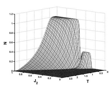
Figure 8: Negativity ${\cal N}_{1,1}$ versus both the exchange interaction coefficient $J_{2}$ and the temperature in four-spin system.

III.2 Numerical results of negativity for more spins

In this section, we present numerical results of negativity for more spins, and first consider the low-temperature case.

III.2.1 Low-temperature case

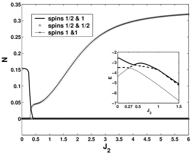
Figure 9: Negativity versus the exchange interaction $J_{2}$ at the temperature $T=0.02$ in six-spin system. The ground and the first two excited energy levels versus the $J_{2}$ are inserted in the plot.

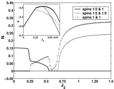
Figure 10: Negativity versus the exchange interaction $J_{2}$ at the temperature $T=0.02$ in eight-spin system, The ground and the first three excited energy levels versus the $J_{2}$ are inserted.

In Fig. 9, we plot the negativity versus $J_{2}$ for the case of six spins at a lower temperature. The negativity ${\cal N}_{1/2,1}$ behaves as a decreasing function of $J_{2}$. It decreases to zero at about $J_{2}=0.27$, which is the special point corresponding to the energy level crossing. On the contrary, around the point $J_{2}=0.27$, ${\cal N}_{1,1}$ jumps up to a nonzero value, and then increases gradually until approaching the limit about ${\cal N}_{1,1}=0.33$. This behavior is quite different from that in the four-spin model.

We also see that ${\cal N}_{1/2,1/2}$ is zero all the time. It can be understood as follows. In the six-site system there are three spin halves with the NNN interaction. Even for a pure homogeneous three-qubit system, there is no entanglement between two spins, irrespective of the strength of the exchange interactions M_Three . Now, in addition to the interaction among three spin halves, there are also interaction between spin halves and spin ones. So, it is reasonable that the entanglement between two spin halves is zero.

The negativity versus $J_{2}$ in the eight-site case is shown in Fig. 10. After the first sharp jump to a value (not zero) at about $J_{2}=0.25$, ${\cal N}_{1/2,1}$ goes down to zero gradually. At approximately $J_{2}=0.55$, the negativity is zero. On the contrary, the negativity ${\cal N}_{1,1}$ jumps up at about $J_{2}=0.25$, and then goes up gradually and almost linearly until $J_{2}$ reaches about $0.55$. Then there happens a sharp decrease to nearly zero, and after that it begins to increase gradually. The negativity ${\cal N}_{1/2,1/2}$ keeps zero until $J_{2}$ reaches about $0.67$, and then it goes up until reaches a steady value.

In Fig. 10, we find that the three kinds of negativity exhibit different properties. From figure inserted, i.e., the energy levels of the eight-spin system, we can see that in the region from about $J_{2}=0.55$ to $J_{2}=0.67$ the first excited energy is quite close to the ground energy. It is known that the energy level crossing can greatly affect the entanglement. Here, the two close energy levels also play an important role in the behavior of entanglement. The approximate degenerate energy levels may remarkably change the probability distribution even at a very low temperature, thereby affect the negativity.

III.2.2 Entanglement versus $J_{2}$ and $T$

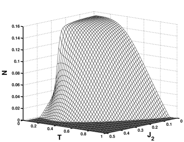
Figure 11: Negativity ${\cal N}_{1/2,1}$ versus both the exchange interaction $J_{2}$ and the temperature in the six-spin system.

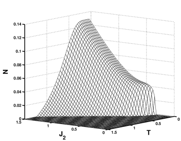
Figure 12: Negativity ${\cal N}_{1,1}$ versus both the exchange interaction $J_{2}$ and the temperature in six-spin system.

Now, we present the entanglement versus $J_{2}$ and $T$ in the six-spin model. The NN negativity ${\cal N}_{1/2,1}$ is shown in Fig. 11. On the $J_{2}-T$ plane, similar to the four-spin case, the $J_{\text{2th}}$ does not behave as a monotonous function of $T$ and it reaches its maximum at about $T=0.27$. From the figure, we may find that the entanglement only exists in the region approximately $T<0.925$ and $J_{2}<0.418$. The strong NNN interaction and thermal fluctuation will suppress the NN entanglement to zero.

We do not plot the negativity ${\cal N}_{1/2,1/2}$ as it is zero all along for any $J_{2}$ and $T$. We give the NNN negativity ${\cal N}_{1,1}$ in Fig. 12. In the region of $J_{2}<0.282$, there is no negativity ${\cal N}_{1,1}$ at any temperature. The threshold $J_{\text{2th}}$ is increased by the increasing temperature, similar to the four-spin case.

IV conclusion

In conclusion, we have studied the entanglement properties of the (1/2,1) mixed-spin systems described by the Heisenberg model. In the systems only with NN exchange interactions, for two-spin and three-spin cases analytical results of the negativity have been obtained, which facilitate our discussions of entanglement. The analytical expression of threshold temperature after which the entanglement vanishes are obtained for the two-site case. For the case of even number of particles, it has been found that the pairwise thermal entanglement is solely determined by the internal energy, and thus builds an interesting relation between the microscopic quantity, entanglement, and the macroscopic thermal dynamical function, the internal energy in the mixed-spin systems. For the odd number of particles such as the three-site case, we also provide a relation between the internal energy and negativities. We have numerically studied the effects of different finite temperature and magnetic fields on entanglement. As a conclusion, the thermal fluctuation suppresses the entanglement, and entanglement may change evidently at some critical points of magnetic field.

In the systems also with NNN interactions, by applying the angular momentum coupling method, we obtained analytical results of all the eigenenergies of the four-spin system, based on which the negativity of the NN spins has been obtained. We also considered the excited-state entanglement. At finite temperature, from the partition function, the analytical results of negativity has been given. We have numerically studied the effects of the NNN interaction on the NN entanglement and NNN entanglement. It is natural to see that the NNN interaction suppresses the NN entanglement, and enhances the NNN entanglement. We found that the negativity between two spin ones is sensitive to $J_{2}$ and displays some interesting properties. At finite temperature, the thermal fluctuation suppresses both the NN entanglement and the NNN entanglement. The threshold values $J_{\text{2th}}$ and $T_{\text{th}}$ are studied in detail. The entanglement displays some peculiar properties, which are quite different from those of the spin-half model. These are due to inherent mixed-spin character of our system. It is more interesting to study entanglements in other mixed systems and explore some universal properties, which are under consideration.

Appendix A Two-site Heisenberg model with a magnetic field

The Hamiltonian of the two-site Heisenberg model with a magnetic field is written explicitly as

$$H_{1}=s_{1x}\otimes S_{2x}+s_{1y}\otimes S_{2y}+s_{1z}\otimes S_{2z}+B(s_{1z}+S_{2z}).$$

Following the same way as the discussions of subsection II.A, the density matrix of the thermal state is given by Eq. (6) with the matrix elements

$$a_{1}= a_{6}e^{3\beta B}=e^{\frac{\beta}{2}(3B-1)},$$

$$a_{5}= a_{2}e^{\beta B}=\frac{1}{3}e^{\frac{\beta B}{2}}\Big{(}e^{\beta}+2e^{-\frac{\beta}{2}}\Big{)},$$

$$a_{4}= a_{3}e^{\beta B}=\frac{1}{3}e^{\frac{\beta B}{2}}\Big{(}2e^{\beta}+e^{-\frac{\beta}{2}}\Big{)},$$

$$b_{2}= b_{1}e^{\beta B}=-\frac{\sqrt{2}}{3}e^{\frac{\beta B}{2}}\Big{(}e^{\beta}-e^{-\frac{\beta}{2}}\Big{)},$$

and the partition function

$$Z = e^{\frac{\beta}{2}(3B-1)}+e^{-\frac{\beta}{2}(3B+1)}$$ (52)

$$+ e^{\frac{1}{4}\beta}\cosh\big{(}\frac{3\beta}{4}\big{)}\cosh\big{(}\frac{\beta B}{2}\big{)}.$$

Having obtained the analytical expressions of the matrix, we directly obtain the negativity after substituting the matrix elements to Eq. (13).

References

- (1) M. A. Nielsen, Ph. D thesis, University of Mexico, 1998, quant-ph/0011036;
- (2) M. C. Arnesen, S. Bose, and V. Vedral, Phys. Rev. Lett. 87, 017901 (2001).
- (3) D. Gunlycke, V. M. Kendon, V. Vedral, and S. Bose, Phys. Rev. A64, 042302 (2001).
- (4) X. Wang, Phys. Rev. A 64, 012313 (2001).
- (5) X. Wang, H. Fu, and A. I. Solomon, J. Phys. A: Math. Gen. 34, 11307(2001); X. Wang and K. Mølmer, Eur. Phys. J. D 18, 385(2002).
- (6) G. L. Kamta and A. F. Starace, Phys. Rev. Lett. 88, 107901 (2002).
- (7) K. M. O’Connor and W. K. Wootters, Phys. Rev. A63, 0520302 (2001).
- (8) D. A. Meyer and N. R. Wallach, J. Math. Phys. 43, 4273 (2002).
- (9) T. J. Osborne and M. A. Nielsen, Phys. Rev. A66, 032110 (2002).
- (10) A. Osterloh, L. Amico, G. Falci and R. Fazio, Nature 416, 608 (2002).
- (11) Y. Sun, Y. G. Chen, and H. Chen, Phys. Rev. A 68, 044301 (2003).
- (12) L. F. Santos, Phys. Rev. A67, 062306 (2003).
- (13) Y. Yeo, Phys. Rev. A66, 062312 (2002).
- (14) D. V. Khveshchenko, Phys. Rev. B68, 193307 (2003).
- (15) L. Zhou, H. S. Song, Y. Q. Guo, and C. Li, Phys. Rev. A68, 024301 (2003).
- (16) G. K. Brennen, S. S. Bullock, Phys. Rev. A70, 52303 (2004).
- (17) R. Xin, Z. Song, and C. P. Sun, quant-ph/0411177.
- (18) G. Tóth, quant-ph/0406061.
- (19) F. Verstraete, M. Popp, and J. I. Cirac, Phys. Rev. Lett. 92, 027901 (2004).
- (20) F. Verstraete, M. A. Martin-Delgado, J. I. Cirac, Phys. Rev. Lett. 92, 087201 (2004).
- (21) J. Vidal, G. Palacios, and R. Mosseri, Phys. Rev. A 69, 022107 (2004).
- (22) N. Lambert, C. Emary, and T. Brandes, Phys. Rev. Lett. 92, 073602 (2004).
- (23) S. J. Gu, S. S. Deng, Y. Q. Li, and H. Q. Lin, Phys. Rev. Lett. 93, 086402 (2004).
- (24) Y. Chen, P. Zanardi, Z. D. Wang, and F. C. Zhang, quant-ph/0407228.
- (25) S. B. Li and J. B. Xu, Phys. Lett. A 311, 313 (2003).
- (26) K. Audenaert, J. Eisert, M. B. Plenio, and R. F. Werner, Phys. Rev. A66, 042327 (2002).
- (27) L. A. Wu, M. S. Sarandy, and D. A. Lidar, quant-ph/0407056.
- (28) G. Vidal, J. I. Latorre, E. Rico, and A. Kitaev Phys. Rev. Lett. 90, 227902 (2003).
- (29) S. Bose, Phys. Rev. Lett. 91, 207901 (2003); V. Subrahmanyam, Phys. Rev. A69, 034304 (2004); M. Christandl, N. Datta, A. Ekert, and A. J. Landahl, Phys. Rev. Lett. 92, 187902 (2004); Y. Li, T. Shi, Z. Song, and C. P. Sun, quant-ph/0406159; M. B. Plenio and F. L Semião, quant-ph/0407034.
- (30) W. K. Wootters, Phys. Rev. Lett. 80, 2245 (1998).
- (31) J. Schliemann, Phys. Rev. A68, 012309 (2003).
- (32) L. Zhou, X. X. Yi, H. S. Song, and Y. Q. Guo, quant-ph/0310169.
- (33) Y. Q. Li and G. Q. Zhu, submitted.
- (34) A. Peres, Phys. Rev. Lett. 77, 1413 (1996); M. Horodecki, P. Horodecki, and R. Horodecki, Phys. Lett. A 223, 1 (1996).
- (35) G. Vidal and R. F. Werner, Phys. Rev. A65, 032314 (2002).
- (36) I. Bose and E. Chattopadhyay, Phys. Rev. A 66, 062320 (2002).
- (37) S. J. Gu, H. B. Li, Y. Q. Li, and H. Q. Lin, Phys. Rev. A 70, 052302 (2004).
- (38) X. Wang, Phys. Lett. A 329, 439 (2004).
- (39) X. Wang and P. Zanardi, Phys. Lett. A 301, 1 (2002).