Information transmission via entangled quantum states
in Gaussian channels with memory

Abstract

Gaussian quantum channels have recently attracted a growing interest, since they may lead to a tractable approach to the generally hard problem of evaluating quantum channel capacities. However, the analysis performed so far has always been restricted to memoryless channels. Here, we consider the case of a bosonic Gaussian channel with memory, and show that the classical capacity can be significantly enhanced by employing entangled input symbols instead of product symbols.

1 Introduction

The evaluation of information capacities of quantum communication channels is of great interest in quantum information theory. In particular, an important question is to determine how much classical information can be processed asymptotically via a quantum channel. This problem has been solved, today, only for a few quantum channels, and it has been addressed only recently for bosonic channels, i.e., continuous-variable quantum channels acting on a bosonic field such as the electromagnetic field [1]. The classical capacity of a purely lossy bosonic channel was solved exactly very recently [2], while the case of noisy bosonic channels is already more involved. Actually, the classical capacity of the Gaussian bosonic channel, i.e., a continuous-variable quantum channel undergoing a Gaussian-distributed thermal noise, has been derived in [3] although this result only holds provided that the optimal input ensemble is a tensor product of Gaussian states, as conjectured by several authors but not rigorously proven today (see e.g. [4] for recent progress on this problem). All these studies, however, have been restricted to memoryless bosonic channels.

The first analysis of the classical capacity of quantum channels with memory was performed in [5]. In this work a qubit depolarizing channel with memory was investigated and the first evidence that entangled input states enhance the single-shot capacity was provided. It was shown that the single-shot capacity is always maximized either by product states or by maximally entangled states at the input, and that the product versus entangled states optimal regime depends on a threshold value for the degree of channel memory. This threshold value turned out to be a function of the depolarization factor of the channel. The same features mentioned above for the depolarizing channel with memory were also later proved for a class of non-isotropic qubit channels with memory [6].

In this paper, we investigate the capacity of a bosonic Gaussian channel that exhibits memory. We review the main results that were first presented in [7] and provide more details about their derivation. We consider channels with a thermal noise that has a finite bandwidth. The resulting memory effect is modeled by assuming that the noise affecting two subsequent uses of the channel follows a bivariate Gaussian distribution with a non-vanishing correlation coefficient, measuring the degree of memory of the channel. We prove that if the memory is non-zero and if the input energy is constrained, then the channel capacity can be significantly enhanced by using entangled symbols instead of product symbols. The relation between the degree of memory and the resulting optimal input entanglement is analyzed.

The paper is organized as follows. In Sect. 2 we review the description and known results about memoryless bosonic Gaussian channels. In Sect. 3 we introduce the role of memory, and analyse the capacity by allowing the transmission of entangled input states. Finally, in Sect. 4 we summarise and discuss our results.

2 Memoryless Bosonic Gaussian channels

Let us define a memoryless bosonic Gaussian channel $T$ acting on a mode of the electromagnetic field associated with the annihilation and creation operators $a$ and $a^{\dagger}$, or, equivalently, the quadrature components $q=(a+a^{\dagger})/\sqrt{2}$ and $p=i(a^{\dagger}-a)/\sqrt{2}$, satisfying the commutation relation $[q,p]=i$. If the input of the channel is initially in state $\rho$, we have

$$\rho\mapsto T[\rho]=\int d^{2}\beta\ q(\beta)\ D(\beta)\rho D^{\dagger}(\beta),$$ (1)

where $d^{2}\beta=d\Re(\beta)\,d\Im(\beta)$, while $D(\beta)=e^{\beta a^{\dagger}-\beta^{*}a}$ denotes the displacement operator (such that $|\alpha\rangle=D(\alpha)|0\rangle$ with $|0\rangle$ being the vacuum state and $|\alpha\rangle$ being a coherent state of mean value $\alpha$). For a Gaussian channel, the kernel is a bivariate Gaussian distribution with variance $N$, namely

$$q(\beta)=\frac{1}{\pi N}\,e^{-\frac{|\beta|^{2}}{N}}\;.$$ (2)

The channel then randomly displaces an input coherent state according to a Gaussian distribution, which results in a thermal state ($N$ is the variance of the added noise on the quadrature components $q$ and $p$, or, equivalently the number of thermal photons added by the channel). The Gaussian CP map effected by this channel can also be characterized via the covariance matrix. Restricting to Gaussian states with a vanishing mean value, a complete state characterization is provided by the covariance matrix

$$\gamma = \left(\begin{array}[]{cc}\langle q^{2}\rangle&\frac{1}{2}\langle qp+pq\rangle\\ \frac{1}{2}\langle qp+pq\rangle&\langle p^{2}\rangle\end{array}\right).$$ (5)

The Gaussian channel can then be written as

$$\gamma\mapsto\gamma+\left(\begin{array}[]{cc}N&0\\ 0&N\end{array}\right).$$ (6)

The coding theorem for quantum channels asserts that the one-shot classical capacity of a quantum channel $T$ is given by

$$C_{1}(T)=\max\left[S\left(\sum_{i}p_{i}T[\rho_{i}]\right)-\sum_{i}p_{i}S\left(T[\rho_{i}]\right)\right],$$ (7)

where $S(\rho)=-\textrm{Tr}(\rho\log\rho)$ is the von Neumann entropy of the density operator $\rho$. In Eq. (7), the maximum is taken over all probability distributions $\{p_{i}\}$ and collections of density operators $\{\rho_{i}\}$ satisfying the energy constraint

$$\sum_{i}p_{i}\textrm{Tr}\left(\rho_{i}a^{\dagger}a\right)\leq\bar{n},$$ (8)

with $\bar{n}$ being the maximum mean photon number at the input of the channel. For a monomodal bosonic Gaussian channel, it is conjectured that a Gaussian mixture of coherent states (i.e., a thermal state) achieves the channel capacity [8]. The sum over $i$ is replaced by an integral over $\alpha$, where the input states

$$\rho_{\alpha}^{\textrm{in}}=|\alpha\rangle\langle\alpha|$$ (9)

are drawn from the probability density

$$p(\alpha)=\frac{1}{\pi\bar{n}}\,e^{-\frac{|\alpha|^{2}}{\bar{n}}}.$$ (10)

Thus, the one-shot classical capacity of the channel becomes

$$C_{1}(T)=S\left(\bar{\rho}\right)-\int d^{2}\alpha\,p(\alpha)\,S\left(\rho_{\alpha}^{\textrm{out}}\right),$$ (11)

where we have defined the individual output states

$$\rho_{\alpha}^{\textrm{out}}=T[\rho_{\alpha}^{\textrm{in}}]=\frac{1}{\pi N}\int d^{2}\beta\,e^{-\frac{|\beta-\alpha|^{2}}{N}}\,|\beta\rangle\langle\beta|$$ (12)

and their mixture (saturating the energy constraint)

$$\bar{\rho}=\int d^{2}\alpha\,p(\alpha)\,\rho_{\alpha}^{\textrm{out}}=\frac{1}{\pi(\bar{n}+N)}\int d^{2}\beta\,e^{-\frac{|\beta|^{2}}{\bar{n}+N}}\,|\beta\rangle\langle\beta|.$$ (13)

In order to calculate the entropy of a Gaussian state $\rho$, one computes the symplectic values of its covariance matrix $\gamma$, i.e., the solutions of the equation $\left|\gamma-\lambda J\right|=0$, where

$$J=\left(\begin{array}[]{cc}0&i\\ -i&0\end{array}\right).$$ (14)

It can be shown that these values always come as a pair $\pm\lambda$, so that the entropy is given by $S(\rho)=g\left(|\lambda|-\frac{1}{2}\right)$, where

$$g(x)=\left\{\begin{array}[]{ll}(x+1)\log_{2}(x+1)-x\log_{2}x,&x>0\\ 0&x=0\end{array}\right.$$ (15)

is the entropy of a thermal state with a mean photon number of $x$. Since the input states $\rho_{\alpha}^{\textrm{in}}$ are coherent states with a covariance matrix

$$\gamma^{\textrm{in}}=\frac{1}{2}\left(\begin{array}[]{cc}1&0\\ 0&1\end{array}\right),$$ (16)

the individual output states $\rho_{\alpha}^{\textrm{out}}$ and their mixture $\bar{\rho}$ are associated with the covariance matrices

$$\gamma^{\textrm{out}} = \frac{1}{2}\left(\begin{array}[]{cc}1+2N&0\\ 0&1+2N\end{array}\right),$$ (19)

$$\bar{\gamma} = \frac{1}{2}\left(\begin{array}[]{cc}1+2(\bar{n}+N)&0\\ 0&1+2(\bar{n}+N)\end{array}\right),$$ (22)

so that the one-shot capacity of the channel is

$$C_{1}(T)=g(\bar{n}+N)-g(N).$$ (23)

3 Bosonic Gaussian channels with memory

3.1 Multimodal Gaussian states

Let us now generalize these notions to multimodal channels. Similarly to the monomodal case, $s$ modes of the electromagnetic field, numbered from $1$ to $s$, are associated to $s$ pairs of annihilation and creation operators $a_{j}$ and $a^{\dagger}_{j}$ or, equivalently, of quadrature components $q_{j}$ and $p_{j}$. Ordering these observables in a column vector

$$R=[q_{1},p_{1},\ldots,q_{s},p_{s}]^{\textrm{T}},$$ (24)

we define the mean vector $m^{(s)}$ and the covariance matrix $\gamma^{(s)}$ of an $s$-mode state $\rho^{(s)}$ as

$$m^{(s)} = \textrm{Tr}\ \rho^{(s)}R,$$ (25)

$$\gamma^{(s)} = \textrm{Tr}\ (R-m^{(s)})\rho(R-m^{(s)})^{\textrm{T}}-\frac{1}{2}\bigoplus_{j=1}^{s}J_{j},$$ (26)

where each $J_{j}$ takes the form (14). We now focus on Gaussian states, which are completely specified by their mean vector and covariance matrix. The von Neuman entropy of such a state is then given by

$$S(\rho^{(s)})=\sum_{j=1}^{s}g\left(|\lambda_{j}|-\frac{1}{2}\right),$$ (27)

where $\pm\lambda_{j}$ are the symplectic eigenvalues of the covariance matrix $\gamma^{(s)}$ of the state; that is the solutions of the equation

$$\left|\gamma^{(s)}-\lambda\bigoplus_{j=1}^{s}J_{j}\right|=0.$$ (28)

This will allow us to compute the one-shot classical capacity of bosonic Gaussian channels acting on $s$ modes [8], since this will still take the form (7), but with a generalized energy constraint

$$\frac{1}{s}\sum_{j=1}^{s}\sum_{i}p_{i}\textrm{Tr}\left(\rho_{i}^{(s)}a_{j}^{\dagger}a_{j}\right)\leq\bar{n}.$$ (29)

3.2 Memoryless bimodal channel

Consider two subsequent uses of a memoryless channel $T$, defining the bimodal channel

$$\rho\mapsto T_{12}[\rho]=\int d^{2}\beta_{1}\ d^{2}\beta_{2}\ q(\beta_{1},\beta_{2})$$ (30)

$$\times D(\beta_{1})\otimes D(\beta_{2})\;\rho\;D^{\dagger}(\beta_{1})\otimes D^{\dagger}(\beta_{2}),$$

where

$$q(\beta_{1},\beta_{2})=\frac{1}{\pi^{2}N^{2}}e^{-\frac{|\beta_{1}|^{2}+|\beta_{2}|^{2}}{N}}$$ (31)

since the noise affecting the two uses is uncorrelated. Following Eqs. (24-26), we define the covariance matrix $\gamma_{12}$ of a bimodal state $\rho_{12}$. We restrict ourselves to bimodal Gaussian states [8], characterized by

$$\gamma_{12}=\left(\begin{array}[]{cc}\gamma_{1}&\sigma_{12}\\ \sigma_{12}^{\mathrm{T}}&\gamma_{2}\end{array}\right),$$ (32)

where $\gamma_{1}$ is the covariance matrix associated with the reduced density operator $\rho_{1}=\textrm{Tr}_{2}(\rho_{12})$ of mode $1$ (and similarly for $\gamma_{2}$), while $\sigma_{12}$ characterizes the correlation and/or entanglement between the two modes. For a memoryless channel, the optimal input states are simply products of coherent states, with a covariance matrix $\gamma_{12}^{\textrm{in}}=\gamma_{1}^{\textrm{in}}\oplus\gamma_{2}^{\textrm{in}}$ where $\gamma_{1}^{\textrm{in}}$ and $\gamma_{2}^{\textrm{in}}$ both take the form (16), while $\sigma_{12}^{\textrm{in}}=0$. The optimal input modulation is a product of Gaussian distributions,

$$p(\alpha_{1},\alpha_{2})=\frac{1}{\pi^{2}\bar{n}^{2}}e^{-\frac{|\alpha_{1}|^{2}+|\alpha_{2}|^{2}}{\bar{n}}}.$$ (33)

It follows that the classical capacity of this channel is additive $\frac{1}{2}\times C_{1}(T_{12})=C_{1}(T)$.

3.3 Bimodal channel with correlated noise

Let us investigate what happens if the noise is correlated, for instance when the two uses are closely separated in time and the channel has a finite bandwidth. We assume that the noise distribution takes the general form

$$q(\beta_{1},\beta_{2})=\frac{1}{\pi^{2}\sqrt{|\gamma^{N}|}}e^{-\bm{\beta}^{\dagger}{\gamma^{N}}^{-1}\bm{\beta}},$$ (34)

where $\bm{\beta}=[\Re(\beta_{1}),\Im(\beta_{1}),\Re(\beta_{2}),\Im(\beta_{2})]^{\textrm{T}}$ and $\gamma^{N}$ is the covariance matrix of the noise quadratures, chosen to be

$$\gamma^{N}=\left(\begin{array}[]{cccc}N&0&-xN&0\\ 0&N&0&xN\\ -xN&0&N&0\\ 0&xN&0&N\end{array}\right).$$ (35)

Thus, the map $T_{12}$ can be expressed by $\gamma_{12}\mapsto\gamma_{12}+\gamma^{N}$, so that the noise terms added on the $p$ quadratures of modes 1 and 2 are correlated Gaussians with variance $N$, while those added on the $q$ quadratures are anticorrelated Gaussians with variance $N$. In Sect. 3.4, we will see that the beneficial effect of entanglement disappears in a more symmetric noise model where the $q$ and $p$ noise quadratures are both correlated. The correlation coefficient $x$ ranges from $x=0$ for a memoryless channel to $x=1$ for a channel with full memory.

We now come to the central result of this paper. While we have seen that for a memoryless channel, the capacity is attained for product states, we will prove that for correlated thermal noise, the capacity is achieved if some appropriate degree of entanglement is injected at the input of the channel. Intuitively, if we take an EPR state, i.e., the common eigenstate of $q_{+}=(q_{1}+q_{2})/\sqrt{2}$ and $p_{-}=(p_{1}-p_{2})/\sqrt{2}$, it is clear that the noise on $q_{+}$ and $p_{-}$ effected by the channel is reduced as $x$ increases. This suggests that using entangled input states may decrease the effective noise, hence increase the capacity. However, EPR states have infinite energy so they violate the energy constraint. Instead, we may inject (finite-energy) two-mode vacuum squeezed states, whose covariance matrix is given by

$$\gamma_{1}^{\textrm{in}} = \gamma_{2}^{\textrm{in}}=\frac{1}{2}\left(\begin{array}[]{cc}\cosh 2r&0\\ 0&\cosh 2r\end{array}\right),$$ (38)

$$\sigma_{12}^{\textrm{in}} = \frac{1}{2}\left(\begin{array}[]{cc}-\sinh 2r&0\\ 0&\sinh 2r\end{array}\right),$$ (41)

with $r$ being the squeezing parameter. Note that purely classical correlations between the quadratures in the input distribution $p(\alpha_{1},\alpha_{2})$ also help increase the capacity when $x>0$, so we have to check that entanglement gives an extra enhancement in addition to this.

The mean photon number in each mode of the state characterized by Eqs. (38)-(41) is $\sinh^{2}r$, so that the maximum allowed modulation (for a fixed maximum photon number $\bar{n}$) decreases as entanglement increases. Remarkably, there is a possible compromise between this reduction of modulation and the entanglement-induced noise reduction on $q_{+}$ and $p_{-}$. To show this, consider input states with $\sinh^{2}r=\eta\bar{n}$; that is

$$\gamma_{1,2}^{\textrm{in}} = \frac{1}{2}\left(\begin{array}[]{cc}1+2\eta\bar{n}&0\\ 0&1+2\eta\bar{n}\end{array}\right),$$ (44)

$$\sigma_{12}^{\textrm{in}} = \frac{1}{2}\left(\begin{array}[]{cc}-2\sqrt{\eta\bar{n}(1+\eta\bar{n})}&0\\ 0&2\sqrt{\eta\bar{n}(1+\eta\bar{n})}\end{array}\right),$$ (47)

where $\eta$ measures the degree of entanglement and is used to interpolate between a product of vacuum states ($\eta=0$), which can be maximally modulated, and an entangled state ($\eta=1$), for which the entire energy is due to entanglement and no modulation can be applied. At the output of the channel, we get states with a covariance matrix $\gamma_{12}^{\textrm{out}}$ where

$$\gamma_{1,2}^{\textrm{out}} = \frac{1}{2}\left(\begin{array}[]{cc}1+2\eta\bar{n}+2N&0\\ 0&1+2\eta\bar{n}+2N\end{array}\right),$$ (50)

$$\sigma_{12}^{\textrm{out}} = \frac{1}{2}\left(\begin{array}[]{cc}-2\sqrt{\eta\bar{n}(1+\bar{n})}-2xN&0\\ 0&2\sqrt{\eta\bar{n}(1+\bar{n})}+2xN\end{array}\right),$$ (53)

while the mixture $\bar{\gamma}_{12}$ of these states are characterized by

$$\bar{\gamma}_{1,2} = \gamma_{1,2}^{\textrm{out}}+\left(\begin{array}[]{cc}(1-\eta)\bar{n}&0\\ 0&(1-\eta)\bar{n}\end{array}\right),$$ (56)

$$\bar{\sigma}_{12} = \sigma_{12}^{\textrm{out}}+\left(\begin{array}[]{cc}y(1-\eta)\bar{n}&0\\ 0&-y(1-\eta)\bar{n}\end{array}\right),$$ (59)

assuming that the energy constraint is saturated. Here, $y$ stands for the classical input correlation coefficient (to compensate for the noise, the $q$ displacements need to be correlated, and the $p$ displacements anti-correlated).

3.4 Independent channels with phase-sensitive noise

Before evaluating the transmission rate achieved by these states, let us give some intuition about why entangled states could help enhance the transmission rate. More precisely, let us study this channel in a modified basis by considering the transformation

$$\left\{\begin{array}[]{ccc}q_{+}&=&{(q_{1}+q_{2})}/{\sqrt{2}}\\ p_{+}&=&{(p_{1}+p_{2})}/{\sqrt{2}}\end{array}\right.\quad\textrm{and}\quad\left\{\begin{array}[]{ccc}q_{-}&=&{(q_{1}-q_{2})}/{\sqrt{2}}\\ p_{-}&=&{(p_{1}-p_{2})}/{\sqrt{2}}\end{array}\right.$$ (60)

which physically corresponds to a 50/50 beam splitter and maps the $1$ and $2$ modes to the $+$ and $-$ modes. Expressing the covariance matrix $\gamma_{+-}^{N}$ of the noise in this new basis confirms that the noise on the $q_{+}$ and $p_{-}$ quadratures is reduced, while the noise on the $p_{+}$ and $q_{-}$ is enhanced:

$$\gamma_{+-}^{N}=\left(\begin{array}[]{cccc}N(1-x)&0&0&0\\ 0&N(1+x)&0&0\\ 0&0&N(1+x)&0\\ 0&0&0&N(1-x)\end{array}\right).$$ (61)

Moreover, in this basis, the channel introduces no correlation between the $+$ and $-$ modes, so that it acts as a product of two independent (memoryless) monomodal channels. These monomodal channels are phase-sensitive, in contrast to those acting on modes $1$ and $2$, since the variances of the $q$ and $p$ noise quadratures are different. As a consequence, their capacity is achieved by transmitting squeezed states [3], described by covariance matrices

$$\gamma_{+}^{\textrm{in}} = \frac{1}{2}\left(\begin{array}[]{cc}e^{-2r}&0\\ 0&e^{2r}\end{array}\right),$$ (64)

$$\gamma_{-}^{\textrm{in}} = \frac{1}{2}\left(\begin{array}[]{cc}e^{2r}&0\\ 0&e^{-2r}\end{array}\right),$$ (67)

where the squeezing parameter $r$ is, as above, such that $\sinh^{2}r=\eta\bar{n}$. Rotating back this product of squeezed states, corresponding to a diagonal covariance matrix $\gamma_{+-}^{\textrm{in}}=\gamma_{+}^{\textrm{in}}\oplus\gamma_{-}^{\textrm{in}}$, into the original basis, we obtain the two-mode squeezed states with covariance matrix $\gamma_{12}^{\textrm{in}}$ as defined in Eqs. (44)-(47).

We may also continue studying this channel in the modified basis where all covariance matrices are diagonal. Indeed, the covariance matrix of states at the output of the channel is given by $\gamma_{+-}^{\textrm{out}}=\gamma_{+-}^{\textrm{in}}+\gamma_{+-}^{N}$. As for the mixture of output states, we have used $\eta\bar{n}$ photons for squeezing, so that we are left with $(1-\eta)\bar{n}$ photons for modulation. Distributing this photon number between the quadratures following the affecting noise then leads to a covariance matrix

$$\bar{\gamma}_{+-}=\gamma_{+-}^{\textrm{out}}+\left(\begin{array}[]{cccc}(1+y)(1-\eta)\bar{n}&0&0&0\\ 0&(1-y)(1-\eta)\bar{n}&0&0\\ 0&0&(1-y)(1-\eta)\bar{n}&0\\ 0&0&0&(1+y)(1-\eta)\bar{n}\end{array}\right),$$ (68)

where the parameter $y$ allows to optimize the distribution of the modulation between the quadratures. Up to the basis change, $\bar{\gamma}_{+-}$ is equivalent to the covariance matrix $\bar{\gamma}_{12}$ characterized by Eqs. (50)-(59).

Using this basis, we also easily understand why the transmission rate of a bosonic gaussian channel where the $q$ and $p$ noise quadratures are both correlated (or both anti-correlated) may not be enhanced by using entangled states. Indeed, the covariance matrix of the noise on the $+$ and $-$ modes takes in this case the form

$$\gamma_{+-}^{N}=\left(\begin{array}[]{cccc}N(1-x)&0&0&0\\ 0&N(1-x)&0&0\\ 0&0&N(1+x)&0\\ 0&0&0&N(1+x)\end{array}\right),$$ (69)

which is characteristic of a product of two independent phase-insensitive monomodal channels since the variance of the noise affecting both quadratures of a given mode is the same. The capacity of this channel is thus achieved by transmitting coherent states, which, after the change of basis, remain unentangled states.

3.5 Entanglement-enhanced capacity

In order to evaluate the transmission rate achieved by these states, we need first to compute the symplectic values $\lambda_{12}^{\textrm{out}}$ and $\bar{\lambda}_{12}$ of $\gamma_{12}^{\textrm{out}}$ and $\bar{\gamma}_{12}$, respectively (or, equivalently, of $\gamma_{+-}^{\textrm{out}}$ and $\bar{\gamma}_{+-}$). The symplectic values $\pm\lambda_{12}$ of a covariance matrix $\gamma_{12}$ of the generic form (32) are the solutions of the equation

$$\left|\gamma_{12}-\lambda_{12}(J_{1}\oplus J_{2})\right|=0\;,$$ (70)

or, equivalently, the biquadratic equation

$$\lambda_{12}^{4}-(|\gamma_{1}|+|\gamma_{2}|+2|\sigma_{12}|)\lambda_{12}^{2}+|\gamma_{12}|=0.$$ (71)

Using Eqs. (50)-(59), we see that $\gamma_{12}^{\textrm{out}}$ and $\bar{\gamma}_{12}$ admit each one pair of doubly-degenerate symplectic values, namely

$$\lambda_{12}^{\textrm{out}}=\pm\sqrt{u_{\textrm{out}}^{2}-v_{\textrm{out}}^{2}}\;,\qquad\bar{\lambda}_{12}=\pm\sqrt{\bar{u}^{2}-\bar{v}^{2}}\;,$$ (72)

with

$$u_{\textrm{out}}=\textstyle{\frac{1}{2}}+\eta\bar{n}+N,\hskip 34.14322ptv_{\textrm{out}}=\sqrt{\eta\bar{n}(1+\eta\bar{n})}+xN,$$

$$\bar{u}=\textstyle{\frac{1}{2}}+\bar{n}+N,\quad\bar{v}=\sqrt{\eta\bar{n}(1+\eta\bar{n})}+xN-y(1-\eta)\bar{n}.$$

The transmission rate per mode is then given by

$$R(\eta,y)=g(|\bar{\lambda}_{12}|-\textstyle{\frac{1}{2}})-g(|\lambda_{12}^{\textrm{out}}|-\textstyle{\frac{1}{2}})$$ (73)

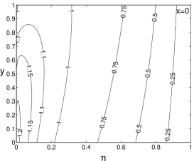
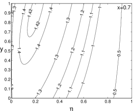
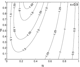
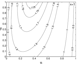
Figure 1: Iso-transmission rate lines in the $(\eta,y)$-plane, where $\eta$ is the degree of entanglement and $y$ is the classical correlation coefficient, for a thermal channel with a degree of memory $x=0$, $0.7$, $0.9$ and $1$. The mean number of photons is $\bar{n}=1$ at the input, while the number of added thermal photons is $N=1/3$.

We may now vary the degree of entanglement $\eta$ and the classical correlation $y$ to maximize the transmission rate $R(\eta,y)$. In Fig. 1, where the level curves of $R(\eta,y)$ for $\bar{n}=1$ and $N=1/3$ are plotted, we see that when there is no memory ($x=0$), the maximum lies at the origin $(\eta_{*},y_{*})=(0,0)$, while the transmission rate decreases as soon as we add classical correlation or entanglement. However, when $x>0$, the maximum is shifted towards non-zero $\eta$ and $y$ values, that is, correlation and entanglement helps increase the transmission rate. For instance, when $x=0.7$, the maximum is attained for $(\eta_{*},y_{*})=(0.19,0.88)$. When the degree of memory $x$ is further increased, the optimal transmission rate is achieved by using maximal classical correlation $y=1$, e. g., for $x=0.9$, we have $(\eta_{*},y_{*})=(0.30,1)$. Nonetheless, as $x$ increases towards $x=1$, the transmission rate may still be enhanced by increasing the degree of entanglement $\eta$. At $x=1$, we have $(\eta_{*},y_{*})=(0.37,1)$.

In Fig. 2, we have plotted the transmission rate $R$ optimized over the classical correlation $y$, as a function of the degree of entanglement $\eta$. When $x>0$, the optimized rate $R$ over $y$ increases with the degree of entanglement $\eta$ and attains a maximum at some optimal value $\eta^{*}>0$. This confirms that entangled input states are useful to enhance the transmission rate provided that the channel exhibits some memory.

Figure 2: Transmission rate $R$ (maximized over the classical correlation coefficient $y$) as a function of the input entanglement $\eta$ for a thermal channel with a degree of memory $x$. The mean number of photons is $\bar{n}=1$ at the input, while the number of added thermal photons is $N=1/3$.

It now suffices to maximize $R$ with respect to both $y$ and $\eta$ in order to find the channel capacity $C$ (assuming that the conjecture [8] is verified and that no product but non-Gaussian states may outperform the Gaussian entangled states considered here). If we keep the signal-to-noise ratio $\bar{n}/N$ constant, it is visible from Fig. 3 that the optimal degree of entanglement $\eta^{*}$ is the highest at some particular value of the mean input photon number $\bar{n}$, and then decreases back to zero in the large-$\bar{n}$ limit (except if $x=0$ or $1$). Clearly, in this limit, the channel $T$ tends to a couple of classical channels with Gaussian additive noise (one for each quadrature), so that entanglement cannot play a role any more [9]. Fig. 4 shows the corresponding optimal value of the input correlation coefficient $y^{*}$ for the same values of the other relevant parameters. Note that, even in the classical limit $\bar{n}\to\infty$, some non-zero input correlation is useful to enhance the capacity of a Gaussian channel with $x>0$.

Figure 3: Optimal degree of input entanglement $\eta^{*}$ as a function of the mean input photon number $\bar{n}$ for a fixed signal-to-noise ratio $\bar{n}/N=3$.

Figure 4: Optimal degree of input correlation $y^{*}$ as a function of the mean input photon number $\bar{n}$ for a fixed signal-to-noise ratio $\bar{n}/N=3$.

4 Conclusion

We have shown that entangled states can be used to enhance the classical capacity of a bosonic channel undergoing a thermal noise with memory. We determined the amount of entanglement that maximizes the information transmitted over the channel for a given input energy constraint (mean photon number per mode) and a given noise level (mean number of thermal photons per mode). For example, the capacity of a channel with a mean number of thermal photons of 1/3 and a correlation coefficient of 70% is enhanced by 10.8% if the mean photon number is 1 and the two-mode squeezing is 3.8 dB at the input. This capacity enhancement may seem paradoxical at first sight since using entangled signal states necessarily decreases the modulation variance for a fixed input energy, which seemingly lowers the capacity. However, due to the quantum correlations of entangled states, the noise affecting one mode can be partly compensated by the correlated noise affecting the second mode, which globally reduces the effective noise. Interestingly, there exists a regime in which this latter effect dominates, resulting in a net enhancement of the amount of classical information transmitted per use of the channel. The capacity gain $G$, measuring the entanglement-induced capacity enhancement, is plotted in Fig. 5. It illustrates that a capacity enhancement of tens of percents is achievable by using entangled light beams with experimentally accessible levels of squeezing. It is interesting to notice that, unlike the qubit channels investigated so far, in the continuous variable case the capacity is always optimized by entangled states by varying the degree of entanglement, and that no threshold on the degree of memory is present.

Figure 5: Capacity gain $G=\max_{y,\eta}R(\eta,y)/\max_{y}R(0,y)$ as a function of the mean input photon number $\bar{n}$ for a fixed signal-to-noise ratio $\bar{n}/N=3$.

References

- [1] A. S. Holevo and R. F. Werner, Phys. Rev. A 63, 032312 (2001).
- [2] V. Giovannetti, S. Guha, S. Lloyd, L. Maccone, J. H. Shapiro, and H. P. Yuen, Phys. Rev. Lett. 92, 027902 (2004).
- [3] A. S. Holevo, M. Sohma, and O. Hirota, Phys. Rev. A 59, 1820 (1999).
- [4] V. Giovannetti, S. Lloyd, L. Maccone, J. H. Shapiro, and B. J. Yen, Phys. Rev. A 70, 022328 (2004); V. Giovannetti, S. Guha, S. Lloyd, L. Maccone, and J. H. Shapiro, Phys. Rev. A 70, 032315 (2004); A. Serafini, J. Eisert, and M. M. Wolf, Phys. Rev. A 71, 012320 (2005).
- [5] C. Macchiavello and G. M. Palma, Phys. Rev. A 65, 050301(R) (2002).
- [6] C. Macchiavello, G.M. Palma and S. Virmani, Phys. Rev. A 69, 010303(R) (2004).
- [7] N.J. Cerf, J. Clavareau, C. Macchiavello and J. Roland, quant-ph/0412089, to appear in Phys. Rev. A (2005).
- [8] In this work, we do not question the generally admitted conjecture that Gaussian states achieve the classical capacity, so we restrict our analysis to Gaussian input states.
- [9] Although the fraction of the input mean photon number that is due to entanglement as , its absolute value tends to a constant (except for ).