Heat Capacity as A Witness of Entanglement

Abstract

We demonstrate that the presence of entanglement in macroscopic bodies (e.g. solids) in thermodynamical equilibrium could be revealed by measuring heat-capacity. The idea is that if the system was in a separable state, then for certain Hamiltonians heat capacity would not tend asymptotically to zero as the temperature approaches absolute zero. Since this would contradict the third law of thermodynamics, one concludes that the system must contain entanglement. The separable bounds are obtained by minimalization of the heat capacity over separable states and using its universal low-temperature behavior. Our results open up a possibility to use standard experimental techniques of solid-state physics – namely, heat capacity measurements – to detect entanglement in macroscopic samples.

I Introduction

Entanglement is not only a fundamental and curious feature of purely quantum nature schroedinger , but it is recognized as a physical resource useful in tasks such as quantum computation, quantum cryptography or reduction of communication complexity. A state $\rho$ of $N$ subsystems is entangled if it cannot be prepared by local operations and classical communication, i.e. it cannot be written as a convex sum over product states: $\rho=\sum_{j}w_{j}\rho^{(1)}_{j}\otimes...\otimes\rho^{(N)}_{j}$, where the factorizable state $\rho^{(1)}_{j}\otimes...\otimes\rho^{(N)}_{j}$ of $N$ individual systems occurs with the weight $w_{j}\geq 0$ $(\sum_{j}w_{j}=1$) in the mixture.

A particularly interesting question is whether or not microscopic phenomena, such as quantum correlations between individual constituents of a macroscopic body (for example, individual spins of a magnetic solid) may affect its macroscopic properties. The usual expectation is that non-classical effects in a macroscopic body vanish due to interaction of its many degrees of freedom with the environment (decoherence). In order to experimentally test this claim, one needs to apply some types of entanglement criteria, such as the Bell inequalities Bell , to macroscopic bodies. Due to limited access to the state of these systems this is, however, usually not possible. Recently, it was shown that some thermodynamical properties, such as the internal energy wang ; qph0406040 ; toth ; dowling ; wu , or the magnetic susceptibility bruknervedralzeil ; wiesniaksusceptibility can detect entanglement between microscopic constituents of the solid. They can hence be used as entanglement witnesses witness . Their additional advantage is their extendibility, that is their proportionality to the size of the sample. For this reason we do not need to know how much of the material is studied, but express the quantities as specific (molar, per site, etc.). However, the two macroscopic quantities mentioned above also have some drawbacks as entanglement witnesses. The magnetic susceptibility can be applied only to magnetic systems and a specific class of Hamiltonians (isotropicwiesniaksusceptibility ). Determining the internal energy at a given temperature might be a complicated experimental task.

In this paper we show how entanglement in macroscopic samples and in thermodynamical equilibrium can be detected by measuring heat capacity. Our method of entanglement detection is both simple and generic. Unlike internal energy, measuring specific heat of a solid is a well-established experimental routine in solid state physics. Furthermore, heat capacity is a generic property of materials and can thus also be measured on non-magnetic systems (in contrast to magnetic susceptibility).

In a more general context, our result shows a new link between two fundamental theories, quantum mechanics and thermodynamics (see Refs. 11-13 for other interesting links between the two theories). It is related to the Nernst’s theorem, also known as the third law of thermodynamics nernst . In the original version, the theorem states that the entropy at the absolute zero temperature is dependent only on the degeneracy of the ground state. Alternatively, it can be expressed as a requirement of unattainability of the absolute zero temperature in a finite number of operations footnote . This requires the specific heat to tend asymptotically to zero as the temperature approaches the absolute zero. We will show, however, that, for certain Hamiltonians and under the assumption that the system is in a separable state, one obtains a non-vanishing value for heat capacity (separable bound) as the temperature approaches the absolute zero. Since this contradicts the third law of thermodynamics one concludes that the system must be in an entangled state. The separable bound for heat capacity is obtained in two different ways, by direct minimization of the value of heat capacity over separable states (the explicit example considered is the Ising model in a transverse magnetic field), and by referring to the universal behavior of heat capacity close to absolute zero. Using these methods we obtain the range of physical parameters (critical temperature and strength of the magnetic field) for which entanglement is present in various classes of systems.

One might question the relevance of our method for entanglement detection since the method requires knowledge of the Hamiltonian of the system, and thus one could directly determine its eigenstates, build thermal states therefrom and check their separability. As we know, computation of eigenstates is in general a hard problem and the origin of some major difficulties in solid state physics. Furthermore, even if the thermal (mixed) state is known, it is in general hard to find out whether it is separable or not. Our method requires only knowledge of eigenvalues (partition function) and can easily be experimentally implemented.

Consider a system descried by a Hamiltonian $H$ to be in a thermodynamical equilibrium at a given temperature $T$. Its thermal state is given by $\rho_{T}=\exp\left(-\frac{H}{kT}\right)/Z$, where $k$ is the Boltzmann constant and $Z=\mbox{Tr}[\exp\left(-\frac{H}{kT}\right)]$ is the partition function. The knowledge of the partition function allows us to derive all thermodynamical quantities. For example, the internal energy is given by $U=-\partial\ln Z/\partial\beta=\mbox{Tr}[H\exp\left(-\frac{H}{kT}\right)]/Z=\mbox{Tr}[\rho_{T}H]$, where $\beta=1/kT$. Similarly, the heat capacity, $C=\partial U/\partial T=1/(kT^{2})\partial^{2}\ln Z/\partial\beta^{2}$, is proportional to the variance of the Hamiltonian,

$$C=\frac{\Delta^{2}(H)}{kT^{2}}=\frac{1}{kT^{2}}(\langle H^{2}\rangle-\langle H\rangle^{2}).$$ (1)

We first consider the particular case of an Ising chain in a transverse magnetic field and then consider a more general case.

II Transverse Ising model

II.1 Introduction

The Hamiltonian of an Ising ring of $N$ spins-$\frac{1}{2}$ in a transverse magnetic field is given by

$$H_{Ising}=J\sum_{i=1}^{N}\sigma_{i}^{z}\sigma_{i+1}^{z}+B\sum_{i=1}^{N}\sigma_{i}^{x},$$ (2)

where we assume the periodic boundary conditions $N+i\equiv i$. Here $B$ is the external transverse magnetic field, and $J$ denotes the coupling constant, taken in this section to be $1$. The Pauli matrices $\sigma_{i}^{j}$ $(j=x,y,z)$ have the following actions on $i$th qubit: $\sigma^{z}_{i}|k_{i}\rangle=(-1)^{k_{i}}|k_{i}\rangle$ and $\sigma^{x}_{i}|k_{i}\rangle=|k_{i}\oplus 1\rangle$ $(k=0,1)$, and $\oplus$ denotes the summation modulo 2.

In the following we will prove that no product state belongs to the eigenbasis of $H_{Ising}$. Therefore, the variance of $H_{Ising}$ and consequently heat capacity, cannot vanish within the set of these states. Since taking a convex sum over product states can only increase the variance, we will conclude that heat capacity cannot vanish for the set of all separable states.

II.2 Proof of non-separability of the eigenstates

The proof that all eigenstates of the Hamlitonian $H_{Ising}$ are entangled is by reductio ad absurdum. We first assume the opposite, i.e. that at least one of the eigenstates is a product state, and then arrive at a contradiction. Suppose that the product state $|\psi\rangle=\otimes_{i=1}^{N}(a_{i}|0_{i}\rangle+b_{i}|1_{i}\rangle)$ is an eigenstate that is associated to the eigenvalue $E$ and $a_{i}\neq 0$ and $b_{i}\neq 0$ for all $i$ (If this was not the case, i.e. $a_{i}=0$ or $b_{i}=0$ for some $i$, $|\psi\rangle$ would not be an eigenstate, because the magnetic field term in $H_{Ising}$ flips the state $|0\rangle$ to $|1\rangle$ and vice versa for every qubit). Under the assumption that $|\psi\rangle$ was an eigenstate with an eigenvalue $E$, the following would need to hold:

$$E=\frac{\langle 00...0|H_{Ising}|\psi\rangle}{\langle 00...0|\psi\rangle}=\frac{\langle 10...0|H_{Ising}|\psi\rangle}{\langle 10...0|\psi\rangle}.$$ (3)

The proof is as follows. The two denominators are equal to $\prod_{i=1}^{N}a_{i}$ and $\frac{b_{1}}{a_{1}}\prod_{i=1}^{N}a_{i}$. Under the action of $H_{Ising}$ onto $|\psi\rangle$ in the expression on the left, only the terms for which either all spins are in the state $|0\rangle$ or for which one spin is in the $|1\rangle$ state and the rest in $|0\rangle$ remain. The numerator on the left is hence equal to $\prod_{i=1}^{N}a_{i}\left(N+B\sum_{i=1}^{N}\frac{b_{i}}{a_{i}}\right)$. Under the action of $H_{Ising}$ onto $|\psi\rangle$ in the expression on the right only the following terms give a contribution: $|10...0\rangle$ (equal to $N-4$), $|0...0\rangle$ and the states in which the first and one other spin are anti-aligned to the rest. The second numerator results in $\prod_{i=1}^{N}a_{i}\left\{\frac{b_{1}}{a_{1}}(N-4)+B\left[1+\frac{b_{1}}{a_{1}}\left(\sum_{i=1}^{N}\frac{b_{i}}{a_{i}}-\frac{b_{1}}{a_{1}}\right]\right)\right\}$. After simplifying both sides of Eq. (3), it reduces to a quadratic equation

$$-B\left(\frac{b_{1}}{a_{1}}\right)^{2}-4\frac{b_{1}}{a_{1}}+B=0.$$ (4)

Note that Eq. (4) has two solutions, some $\frac{b_{1}}{a_{1}}=x_{0}$ and $-\frac{1}{x_{0}}$. Interchanging all bras $\langle 0|$ and $\langle 1|$ in Eq. (3) we arrive to the same form of the equation as Eq. (4), but for the inverse of the fraction, $\frac{b_{1}}{a_{1}}$. This means that also $-x_{0}$ and $\frac{1}{x_{0}}$ must satisfy the equation. This would be true only if $x_{0}=\pm 1$, which is, however, not possible. QED.

II.3 Minimization of the variance of Hamiltonian over separable states

We minimize the variance $\Delta^{2}(H_{Ising})$ over all separable states. To find the minimal value of the variance for all separable states it is sufficient to perform minimization over pure product states only. As shown by Hofmann and Takeuchi hofmanntakeuchi , any convex mixture over product states $\rho=\sum_{i}w_{i}|\phi_{i}\rangle\langle\phi_{i}|$ $(w_{i}\geq 0,\sum_{i}w_{i}=1$ are weights of the product states in the mixture) can only increase the variance of an observable $A$, with respect to the variances $\Delta^{2}(A)_{i}$ of $A$ for individual states $|\phi_{i}\rangle$:

$$\Delta^{2}(A)=\sum_{i}w_{i}\langle(A-\langle A\rangle)^{2}\rangle_{i}=\sum_{i}w_{i}\left(\underbrace{\langle A^{2}\rangle_{i}-\langle A\rangle^{2}_{i}}_{=\Delta^{2}(A)_{i}}+\underbrace{(\langle A\rangle_{i}-\langle A\rangle)^{2}}_{\geq 0}\right)\geq\sum_{i}w_{i}\Delta^{2}(A)_{i},$$

with $\langle A\rangle_{i}=\langle\phi_{i}|A|\phi_{i}\rangle$. This implies that the bound that is obtained for pure product states will also be the bound for all separable (in general, mixed) states.

It can be shown that if the state is a product state, then one has

$$\Delta^{2}(H_{Ising})=\left(N-\sum_{i=1}^{N}\langle\sigma^{z}_{i}\rangle^{2}\langle\sigma^{z}_{i+1}\rangle^{2}+2\sum_{i=1}^{N}\langle\sigma^{z}_{i}\rangle\langle\sigma^{z}_{i+2}\rangle-\sum_{i=1}^{N}\langle\sigma^{z}_{i}\rangle\langle\sigma^{z}_{i+1}\rangle^{2}\langle\sigma^{z}_{i+2}\rangle\right)$$

$$-2B\sum_{i=1}^{N}\langle\sigma^{z}_{i}\rangle\langle\sigma^{z}_{i+1}\rangle(\langle\sigma^{x}_{i}\rangle+\langle\sigma^{x}_{i+1}\rangle)+B^{2}\left(N-\sum_{i=1}^{N}\langle\sigma^{x}_{i}\rangle\right).$$ (5)

Due to the translational symmetry of the system we expect that the product state, which minimizes this expression, is (quasi-)translation invariant. We first consider product states with a period of two sites. In such a state every odd spin is in the same state $|\psi_{1}\rangle$ and, similarly, every even spin is in the state $|\psi_{2}\rangle$. Therefore, the state of $N$ spins ($N$ is here taken even) is $|\psi\rangle=\left(|\psi_{1}\rangle|\psi_{2}\rangle\right)^{\otimes N/2}$ and herein called two-translation invariant. The assumed two-translation invariance of the state allows neighboring spins to have anti-parallel $z$ components – to minimize the interaction energy – and at the same time to have the $x$ components, all anti-aligned to the magnetic field. Since in Eq. (5) one has terms dependent on the correlations between non-neighboring spins, one could expect that the variance should be minimized over states with a period of more than two sites. We have considered four-translation invariant states, $|\psi\rangle=\left(|\psi_{1}\rangle|\psi_{2}\rangle|\psi_{3}\rangle|\psi_{4}\rangle\right)^{\otimes N/4}$ (thus $N$ is divisible by 4) and have shown numerically, that the same bound for the variance is obtained as in the case of two-translational invariant states. We assume that the Bloch vectors of $|\psi_{1}\rangle$ and $|\psi_{2}\rangle$ lie in the $xz$-plane, that is $\forall_{i}$ $\langle\psi_{i}|\sigma^{y}|\psi_{i}\rangle=0$. Under these assumptions the variance takes a form of

$$\Delta^{2}(H_{Ising}) = N\left(1+z_{1}^{2}+z_{2}^{2}-3z^{2}_{1}z_{2}^{2}\right)$$ (6)

$$- 2BN[z_{1}z_{2}(x_{1}+x_{2})]$$

$$+ B^{2}\frac{N}{2}\left(2-x_{1}^{2}-x_{2}^{2}\right),$$

where we have adopted the notation $x_{i}=\langle\psi_{i}|\sigma^{x}|\psi_{i}\rangle=\sin\theta_{i}$ and $z_{i}=\langle\psi_{i}|\sigma^{z}|\psi_{i}\rangle=\cos\theta_{i}$. Since the expression (6) is proportional to $N$, it is convenient to discuss the specific heat capacity, that is the heat capacity per spin.

II.4 Results

Figure 1 presents the results of a numerical minimization of Eq. (6) over $\theta_{1}$ and $\theta_{2}$ as a function of the magnetic field with units of $J=k=1$. The plot confirms that no eigenstate of the Hamiltonian has the proposed form for any $B\neq 0$. In the limit of a very strong field, all spins tend to orient themselves toward the field and build a product state, however, the interaction term contributes the variance with a constant magnitude. This explains why the curve in Fig. 1 does not tend to zero as $B$ increases to infinity, but saturates at $B\approx 3.5$.

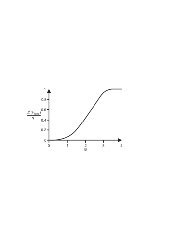
Figure 1: The minimal variance per site $\Delta^{2}(H_{Ising})/N$ of the Hamiltonian of a transverse Ising ring versus the magnetic field $B$ ($J=k=1$). The minimization of the variance is performed over 2-translation invariant product states $\left(|\phi_{1}\rangle|\phi_{2}\rangle\right)^{\otimes N/2}$.

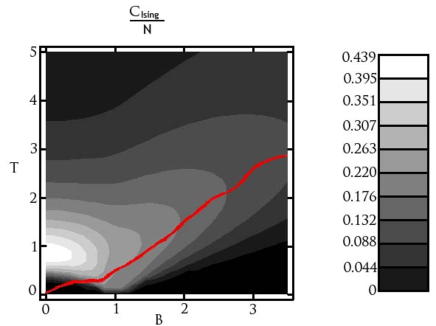
Figure 2: (Color online) The specific heat per spin (in units $|J|=k=1$) of a transverse antiferromagnetic Ising chain versus the temperature $T$ and the magnetic field $B$katsura . The values below the red line indicate the region of the $(T,B)$-space, where entanglement exists. There the variance of the Hamiltonian is lower than for any separable state.

The results of the optimization are compared to the values for specific heat of an infinite Ising ringkatsura . Katsurakatsura obtained analytical forms of thermodynamical quantities by an exact solution of the Hamiltonian eigenproblemkatsura . The solution was achieved with the Jordan-Wigner transformation followed by the Fourier and the Bogoliubov transformations. The heat capacity per spin was found to be

$$\frac{C_{Ising}}{N}=\frac{1}{\pi T^{2}}\int_{0}^{\pi}\frac{f(B,\omega)}{\cosh^{2}\frac{f(B,w)}{T}}d\omega,$$ (7)

where the Boltzmann constant is $k=1$ and $f(B,\omega)=\sqrt{1-2B\cos\omega+B^{2}}$. Figure 2 presents the expression (7) for heat capacity per spin as a function of the external magnetic field and temperature. Values below the red line cannot be explained without entanglement; in this region the $\Delta^{2}(H_{Ising})$ is lower than for any separable state. An interesting observation is that with increasing the strength of the magnetic field, the critical temperature below which entanglement is detected increases as well.

Figure 3 presents the heat capacity per spin for a given magnetic field $B=2$. The gray line represents $a/T^{2}$, where $a=0.4197$ is the minimal Hamiltonian variance over separable states for this value of the field. For the temperatures below the value of intersection of the two lines the state is entangled.

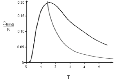
Figure 3: The specific heat per spin (in units $|J|=k=1$) of a transverse antiferromagnetic Ising chain versus the temperature $T$ for $B=2$. The gray line, $0.4197/T^{2}$, is our entanglement witness.

III Universal low-temperature behavior and entanglement

In the following we will show that the specific heat is an entanglement witness, whenever the internal energy is. The argument is based on two results of statistical mechanics, universality and scalability, which together state that the partition functions of various systems are similar and characterized by a small number of universal parameters, such as the central charge or the dimensionality of a lattice.

III.1 Internal energy as entanglement witness

For the sake of the further discussion, we recall that for certain Hamiltonians internal energy is an entanglement witness. This is nicely illustrated in the case of the Heisenberg antiferromagnetic ring Hamiltonian qph0406040 ; toth , given by $H_{xxx}=J\sum_{i=1}^{N}\vec{s}^{i}\cdot\vec{s}^{i+1}$ (with $\vec{s}^{i}$ denoting the $i$-th spin vector of the magnitude $s$ in a ring, periodicity guaranteed by $i\equiv i+N$, and $J>0$). Under optimization over product states $|\psi\rangle=\bigotimes_{i=1}^{N}|\psi_{i}\rangle$, the lowest possible energy is $E_{B}=-JNs^{2}$, since for product states one has:

$$E = \langle\psi|H_{xxx}|\psi\rangle=J\sum_{i=1}^{N}\langle\vec{s}^{i}\rangle\langle\vec{s}^{i+1}\rangle$$ (8)

$$\geq -J\sum_{i=1}^{N}\sqrt{\langle\vec{s}^{i}\rangle^{2}}\sqrt{\langle\vec{s}^{i+1}\rangle^{2}}\geq-JNs^{2}\equiv E_{B}.$$

Here, $\langle\vec{s}^{\!i}\rangle=\langle\psi_{i}|\vec{s}^{i}|\psi_{i}\rangle$.

By convexity, the same bound holds for all separable states. On the other hand, in the limit of large $N$, the ground-state energy per spin, for example, for $s=\frac{1}{2}$ is equal to -0.443$J$ hulthen . Thus, in this case for all temperatures below a critical one ($T_{C}$), for which the internal energy per spin is $U_{xxx,T_{C}}=-0.25J$, the state must contain entanglement.

III.2 Gapless systems

We demonstrate, how the separable bound on the internal energy can be used to derive the separable bound on the heat capacity. First, let us consider a class of materials, in which the lowest part of the energetic spectrum is continuous. Infinite half-odd integer spin chains and ring are examples of such systems. For sufficiently low temperatures, their internal energy (hereafter, “per spin”’) can be expanded to a polynome: $U(T)=E_{0}+(kT)^{\gamma}(c_{0}+c_{1}kT+...)$, with $E_{0}$ being the ground-state energy, and $\gamma,c_{0},c_{1},...$ are material-dependent constants. At sufficiently low temperatures, when the higher order terms are negligible, the specific heat is proportional to a power of $T$ as given by:

$$C(T)=\frac{\partial U(T)}{\partial T}=\gamma c_{0}k^{\gamma}T^{\gamma-1}=\gamma\frac{U-E_{0}}{T}.$$ (9)

Now we use the fact that if the internal energy is bounded for all separable states, i.e., has a separable bound $E_{B}$, then the specific heat is bounded for all separable states as well. Namely, one has

$$C(T)\geq\gamma\frac{E_{B}-E_{0}}{T}.$$ (10)

This allows us to use the heat capacity as entanglement witness. Given a Hamiltonian one determines the ground-state energy $E_{0}$ and the minimal energy over all separable states, $E_{B}$. If the ground state is separable, i.e. $E_{0}=E_{B}$, the inequality (10) is in agreement with the third law of thermodynamics, as one can have $C\rightarrow 0$ with $T\rightarrow 0$. In the case $E_{0}\neq E_{B}$, one compares $\gamma\frac{E_{B}-E_{0}}{T}$ with the real temperature dependence of the heat capacity $C(T)$, obtained either from an experiment or from a theory. Since $\gamma\frac{E_{B}-E_{0}}{T}$ diverges as the temperature approaches the absolute zero and $C(T)$ has to tend to zero to be in an agreement with the third law of thermodynamics, the two curves intersect each other. The intersection point then defines the critical temperature below which entanglement exists in the system. The method does not require the knowledge of the energy eigenstates, but only of the ground state energy and a separable bound for the internal energy.

We note that another thermodynamical entanglement witness has similar features to heat capacity. Namely, the magnetic susceptibity also might diverge in the limit of infinitely low temperatures for all separable states wiesniaksusceptibility . In both cases quantum entanglement is decisive for finiteness of the low-temperature values of the thermodynamical quantities.

Consider gapless models in 1+1 dimensions. For these systems, the conformal field theory Affleck ; blute ; korepin predicts $C=(\pi ck^{2}T)/(3\hbar v)$ for the low-temperature behavior of the specific heat (throughout this paragraph, we assume $J=k=\hbar=1$). Here $c$ stands for the central charge of the corresponding Virasoro algebra and $v$ is the spin velocity. For half-integer spins $c=6s/(2+2s)$. An example is the infinite xxx antiferromagnetic spin-$\frac{1}{2}$ Heisenberg chain. From inequality (10) one obtains that the values of the specific heat below $C<0.386/T$ manifest entanglement in the Heisenberg chain. The approximation $C\approx(2/3)T$ is valid for temperatures below 0.1 xiang .

Another example is the xx spin-$\frac{1}{2}$ antiferromagnets whose solution is also given in Ref. 17. The internal energy per spin of an infinite xx ferromagnet described by the Hamiltonian $H_{xx}=J\sum_{i}(\sigma_{x}^{i}\sigma_{x}^{i+1}+\sigma_{y}^{i}\sigma_{y}^{i+1})$ is given by

$$U_{xx}=-\frac{4J}{\pi}\int_{0}^{\pi/2}\tanh\left(\frac{2J}{kT}\sin\omega\right)\sin\omega d\omega.$$ (11)

We will use the following approximation: at sufficiently low temperatures $T<<k/J$, the argument $\tanh[(2Jx)/(kT)]$ of the integral is a very steep function, which is well approximated by $f(x)=\left(\frac{2J}{kT}\right)x-\left(\frac{J}{kT}\right)^{2}x^{2}$ for $0\leq x\leq\frac{kT}{J}$ and $f(x)=1$ for $x>\frac{kT}{J}$. Thus the internal energy can be written as

$$U_{xx} \approx -\frac{4J}{\pi}\int_{0}^{\frac{kT}{J}}f(\omega)\omega d\omega-\frac{4J}{\pi}\int_{\frac{kT}{J}}^{\frac{\pi}{2}}\sin\omega d\omega$$ (12)

$$\approx -\frac{5k^{2}T^{2}}{3\pi J}-\frac{4J}{\pi}\left(1-\frac{k^{2}T^{2}}{2J^{2}}\right)$$

$$= -\frac{4J}{\pi}+\frac{k^{2}T^{2}}{3\pi J},$$

where we have used expansions $\sin x\approx x$ and $\cos x\approx 1-x^{2}/2$. From Eq. (12) it is clear that the ground-state energy per spin is $-4J/\pi$, while the energy bound for separable states is $-J$. Hence, by Eq. (10) the thermal state is entangled if it satisfies $C<2J(4/\pi-1)/T$ as long as the specific heat can be approximated by a linear function of $T$.

III.3 Gapped systems

The integer spin chains have an energy gap $\Delta$ between the ground state and the first excited state, even in the thermodynamical limit. The gap is also a feature of systems described by a Hilbert space of finite dimensions. For all gapped systems, the low-temperature behavior of the specific heat is given by

$$C=c^{\prime}T^{\delta}e^{-\frac{\Delta}{kT}},$$ (13)

where $c^{\prime}$ and $\delta$ are some material-dependent constants gap . The internal energy can then be written as $U(T)=U_{0}+\int_{0}^{T}C(T^{\prime})dT^{\prime}=U_{0}+c^{\prime}(\Delta/k)^{\delta+1}\Gamma\left[-\delta-1,\Delta/(kT)\right]$. Since for large $x$ we have $\Gamma(a,x)\approx e^{-x}x^{a-1}$ Stegun , we obtain $U(T)\approx E_{0}+c^{\prime}kT^{\delta+2}e^{-\Delta/(kT)}/\Delta$ at sufficiently low temperatures. Finally, using the energy bound $E_{B}$ for separable states we obtain the corresponding bound for the specific heat:

$$C\geq\frac{\Delta(E_{B}-E_{0})}{kT^{2}}$$ (14)

for all separable states. Again, one can invoke the third law of thermodynamics to argue for the necessity of existence of entanglement at sufficiently low temperatures whenever $E_{B}\neq E_{0}$. An exemplary gapped system is an infinite xxx spin-1 Heisenberg chain with the values $c^{\prime}=\Delta^{5/2}/\sqrt{2\pi}$, $\delta=-3/2$, $\Delta=0.411J$, and $E_{0}=-1.401J$ ref32 ; ref33 . By Eq. (8), $E_{B}=-J$. Thus, within the approximation range, all low-temperature values of the specific heat below $0.165J/(kT^{2})$ cannot be explained without entanglement.

IV conclusions

In summary, we have shown that the low-temperature behavior of the specific heat can reveal the presence of entanglement in bulk bodies in the thermodynamical equilibrium. For certain Hamiltonians and under the assumption of having separable states only, the specific heat would diverge at temperature approaching the absolute zero. This might be because none of the eigenstates of the Hamiltonian are a product state and hence its variance cannot vanish within the set of these states or, more generally, because at least the ground state is entangled. In the latter case we involve the separability bound and the universal low-temperature behavior of internal energy to argue for non-classicality of a thermal mixture in certain systems. One may therefore say that in these systems the validity of the third law of thermodynamics relies on quantum entanglement.

Thermal entanglement of bulk solids might play an important role in the emerging quantum information technology, where non–classical correlations were recognized as one of its main resources nielsen . Our method enables to detect entanglement using one of the standard techniques in solid-state physics – measurements of the heat capacity.

V Acknowledgements

We thank J. Kofler for valuable remarks. Č.B. acknowledges support of the Austrian Science Foundation (FWF), Doctorial Programe ”Complex Quantum Systems (QoCuS), and the European Commission (QAP). M.W. is supported by the Erwin Schrödinger Institute in Vienna and the Foundation for Polish Science (FNP) (including scholarship START). This work is partially supported by the National Research Foundation and Ministry of Education, Singapore.

References

- (1) E. Schröedinger, Naturwissenschaften 23, 807 (1935); 23, 823; 23, 844 (1935).
- (2) J. S. Bell, Physics (Long Island City, N.Y.) 1, 195 (1964).
- (3) X. Wang, Phys. Rev. A 66, 034302 (2002).
- (4) Č. Brukner and V. Vedral, quant-ph/0406040 @ www.arxiv.org.
- (5) G. Toth, Phys. Rev. A 71, 010301(R) (2005).
- (6) M. R. Dowling, A. C. Doherty, S. D. Bartlett, Phys. Rev. A 70, 062113 (2004).
- (7) L.-A. Wu, S. Bandyopadhyay, M. S. Sarandy, D. A. Lidar, Phys Rev. A 72 032309 (2005).
- (8) Č. Brukner, V. Vedral, and A. Zeilinger, Phys. Rev. A 73, 012110 (2006).
- (9) M. Wieśniak, V. Vedral, C. Brukner, N. Jour. Phys. 7, 258 (2005).
- (10) M. Horodecki, P. Horodecki, and R. Horodecki. Phys. Lett. A 223, 1 (1996).
- (11) A. Landé, Phys. Rev. 87, 267 (1952).
- (12) A. Peres, in Quantum Theory: Concepts and Methods, Springer (1993).
- (13) A. Peres, Phys. Rev. Lett. 63, 1114 (1989).
- (14) W. Nernst, Sitzber. Preuss. Akad. Wiss. Physik-mat. Kl., 134 (1912).
- (15) Full equivalence of these two formulations is widely discussed, for example in [P.T. Landsberg, Am. J. Phys. 65, 296 (1997) and references therein]. A convincing argument that unattainability of absolute zero is implied by Nernst’s theorem is given in [E. A. Guggenheim, Thermodynamics. An advanced treatment for chemists and physicists. North Holland, Amsterdam (1949)] and based on the fact that (for finite-dimensional systems) entropy must be also finite, which puts a restriction that . The converse implication is discussed in e.g. [A. Münster, Statistical Thermodynamics. Vol. 2, Academic Press, New York, (1974)] under some assumptions.
- (16) H.F. Hofmann, and S. Takeuchi, Phys. Rev. A 68, 032103 (2003).
- (17) S. Katsura, Phys. Rev. 127, 1508 (1962).
- (18) L. Hultén, Arikv Math. Astron. Fys., 26A, 1 (1938).
- (19) I. Affleck, Phys. Rev. Lett. 56, 746 (1986)
- (20) H. W. J. Blöte, J.L. Cardy, M. P. Nightingale, Phys. Rev. Lett. 56, 742 (1986).
- (21) V. E. Korepin, Phys. Rev. Lett., 92, 096402 (2004).
- (22) T. Xiang, Phys. Rev. B 58, 9142 (1998).
- (23) F. Haldane, Phys. Lett. A, 93, 464 (1983).
- (24) M. Abramowitz and I. Stegun, Handbook of Mathematical Functions, Dobler Publ. (N. Y., 1964).
- (25) T. Jolicoeur and O. Golinelli, Phys. Rev. B 50, 9265 (1994).
- (26) S. R. White, D.A. Huse, Phys. Rev. B 48 3844 (1993).
- (27) M. A. Nielsen, and I. L. Chuang Quantum Computation and Quantum Information (Cambridge University, 2000).